Safe Hybrid-Action Reinforcement Learning-Based Decision and Control for Discretionary Lane Change

Abstract

Autonomous lane-change, a key feature of advanced driver-assistance systems, can enhance traffic efficiency and reduce the incidence of accidents. However, safe driving of autonomous vehicles remains challenging in complex environments. How to perform safe and appropriate lane change is a popular topic of research in the field of autonomous driving. Currently, few papers consider the safety of reinforcement learning in discretionary lane-change scenarios. We introduce safe hybrid-action reinforcement learning into discretionary lane change for the first time and propose the Parameterized Soft Actor–Critic with PID Lagrangian (PASAC-PIDLag) algorithm. Furthermore, we conduct a comparative analysis with Parameterized Soft Actor–Critic (PASAC), which is an unsafe version of PASAC-PIDLag. Both algorithms are employed to train the lane-change strategy to output both discrete lane-change decisions and continuous longitudinal vehicle acceleration. Our simulation results indicate that at a traffic density of 15 vehicles per kilometer (15 veh/km), the PASAC-PIDLag algorithm exhibits superior safety with a collision rate of 0%, outperforming the PASAC algorithm, which has a collision rate of 1%. The generalization assessments reveal that at low traffic density levels, both the PASAC-PIDLag and PASAC algorithms are proficient in attaining zero collision rates. However, at high traffic density levels, although both algorithms result in collisions, PASAC-PIDLag has a much lower collision rate than PASAC.

1. Introduction

Nowadays, lane changing is a challenging task that necessitates precise maneuvers to ensure it is conducted safely, comfortably, and swiftly. Lane change include both mandatory and discretionary scenarios [1]. Mandatory lane change refer to the motion planning of lane changing in situations where it is imperative to do so. Scenarios for mandatory lane change include merging from entrance ramps and changing lanes in the presence of obstacles ahead [2]. Discretionary lane change are decisions made by a vehicle to change lanes when it is not demanded due to road conditions, but rather motivated by factors such as speed optimization, driving efficiency, or driver preference. Unlike mandatory lane change, which occur because of immediate necessities such as road obstructions, construction, or merging, discretionary lane change offer an additional layer of complexity to autonomous vehicle algorithms.

Current scholars have provided two research methodologies for decision making in autonomous vehicle lane change: (1) rule-based methods [3,4,5,6] and (2) learning-based methods [7,8].

Rule-based decision models use a set of predefined, hand-crafted rules to simulate the decision-making process of drivers. These rules may include adherence to traffic regulations, such as stopping at red lights and proceeding at green lights. The model is highly interpretable because the rules are clear and straightforward, making them easy to understand and maintain. However, rule-based models may lack flexibility when dealing with complex driving environments and unknown situations because hand-crafted rules may not easily adapt to such complexities and uncertainties [3,6].

Learning-based decision models rely on training models on large-scale driving data to autonomously learn and adapt to different driving conditions. These methods employ deep learning techniques that utilize neural networks and machine learning algorithms to address complex driving decision problems. Although this approach excels in adapting to varied driving scenarios, it has relatively poor interpretability, and there is little guarantee of safety.

Most current learning-based articles are dedicated to using deep reinforcement learning techniques for discretionary autonomous lane-change control of self-driving vehicles [9,10,11,12,13,14]. In [9], the authors proposed a framework that integrates deep reinforcement learning with Q-masking to enhance the efficiency of autonomous lane change. In [8], the authors enhanced the efficiency of the deep Q-learning algorithm and applied it to the autonomous lane-change scenario [15]. In [10], the authors introduced an automated lane-change method based on reinforcement learning, designing a Q-function approximator with a closed-form greedy policy capable of achieving smooth and efficient driving strategies in various and unpredictable scenarios. In [11], the authors developed a deep reinforcement learning agent capable of robustly executing automated lane change in dynamic and uncertain highway environments, demonstrating superior performance over traditional heuristic-based methods. In [12], the authors applied deep reinforcement learning to address the challenge of successful merging or lane changing for autonomous vehicles in high-density traffic, establishing a benchmark for driving in high-density traffic conditions.

The majority of the literature currently employs discrete reinforcement learning for implementing autonomous lane change [8,9,10,11,12,13,14], where the high-level control outputs lane-change decisions using discrete reinforcement learning, and the low-level control uses car-following models such as the Intelligent Driver Model (IDM) [16] to output vehicle acceleration. The decision-making and motion-planning modules, as two closely adjacent and important functional modules of autonomous vehicles, are highly interrelated in terms of functionality and ultimate performance. Therefore, the design of the decision-making process should take into account the feasibility of motion planning. Likewise, motion planning should be formulated based on the decision made [17]. Therefore, in our work, we have adopted a hybrid action space to simultaneously address discrete lane-change decisions and continuous longitudinal acceleration control.

To apply deep reinforcement learning to the autonomous lane-change scenario, ensuring the safety of decision making is essential. There is a paucity of literature considering the safety aspects of autonomous lane change. Given the absence of research using safe reinforcement learning to ensure the safety of discretionary lane change, our paper uses the PID Lagrangian-based hybrid-action reinforcement learning approach [18] to implement autonomous lane change. In [19], the authors proposed a decision-making framework for autonomous vehicles in lane-change scenarios based on deep reinforcement learning with risk awareness. In [20], the authors used a human-driving lane-change decision model combined with regret theory to improve the safety and efficiency of autonomous vehicles in mixed traffic. In [21], the authors introduced a safe reinforcement learning algorithm into the field of autonomous driving, combining the Proximal Policy Optimization (PPO) algorithm with a PID Lagrangian approach to enhance the traffic compliance of motion planners for self-driving vehicles [22].

Safe reinforcement learning [23] is a type of reinforcement learning that incorporates the concepts of safety or risk. Specifically, safe reinforcement learning emphasizes not only pursuing long-term maximum returns during the learning and implementation phases but also adhering to established safety constraints while ensuring reasonable system performance. Compared to Constrained Policy Optimization (CPO) algorithms [24] and safe reinforcement learning algorithms based on Lyapunov functions [25], the Lagrangian-based safe reinforcement learning algorithm performed equally well or even better in tests within the Safety Gym environment [26]. The oscillations and overshooting observed during the learning process can lead to constraint violations by the agent when applied in practice. Therefore, the PID-based Lagrangian method was proposed [18]. From a control perspective, traditional Lagrange multiplier updates behave as integral control, whereas the PID-based approach introduces proportional and differential controls to stabilize the learning process of the agent.

To the best of our knowledge, there are no existing studies that apply safe hybrid action space algorithms in the domain of discretionary lane change. Previous works have applied hybrid-action reinforcement learning to the discretionary lane-change scenario but have not considered safety [27,28,29,30]. In [31], the authors adopted the safe proximal policy optimization algorithm to train the mandatory lane-change policy of an autonomous vehicle. Although the algorithm was designed with safety in mind, the lane-change strategy still exhibited a collision rate of 0.5% in the simulation tests.

The contribution of this paper includes the introduction of a novel safe hybrid-action reinforcement learning algorithm, PASAC-PIDLag, and its application to the discretionary lane-change scenario. We conducted a comprehensive and quantitative comparison between PASAC-PIDLag and its unsafe version PASAC, demonstrating that PASAC-PIDLag outperforms PASAC in terms of both safety and optimality.

Regarding the structure of the paper, Section 2 presents the PASAC-PIDLag and PASAC algorithms, Section 3 discusses the application of the algorithms to lane-change scenarios, Section 4 presents the experiments and results, and Section 5 presents the conclusions.

2. Reinforcement Learning Preliminaries

Reinforcement learning is a computational approach to learning from interaction. In this paradigm, an agent takes actions based on the current state of the environment at each time step. As a result, the environment transitions to another state in the next time step, and the agent receives a reward based on the action taken. Both the actions taken by the agent and the rewards provided by the environment are probabilistic. The goal of an RL algorithm is to maximize the expected discounted cumulative reward.

The framework used to model the environment and the agent’s interactions within it in RL is the Markov Decision Process (MDP). An MDP is defined as a tuple $(S,A,R,P,\gamma )$, where S is a finite set of states of the environment. A is a finite set of actions that the agent can choose from. P is the state-transition probability matrix. $P\left(s^{\prime }\right|s,a)$ represents the probability of transitioning from state s to state $s^{\prime }$ after the agent takes action a. R is a reward function. $R(s,a)$ represents the immediate reward the agent receives after taking action a in state s. $\gamma$ is the discount factor, typically within the range $0\le \gamma \le 1$, which determines the present value of future rewards.

The agent’s objective is to discover a policy $\pi$, which maps states to the probabilities of selecting each possible action, denoted as $\pi :S\to A$, that maximizes the expected sum of discounted rewards. The optimal policy ${\pi }^{*}$ can be formally defined as:

$${\pi }^{*}=arg\underset{\pi }{max}\mathbb{E}\left[{\displaystyle \sum _{t=0}^{\infty }}{\gamma }^{t}R(s_t,a_t)|s_0=s,a_t=\pi \left(s_t\right)\right],$$

(1)

2.1. Soft Actor–Critic

The Soft Actor–Critic (SAC) algorithm [32] is an off-policy, actor–critic reinforcement learning algorithm that incorporates the principles of entropy maximization to balance exploration and exploitation. SAC employs two types of neural networks: soft Q-networks that approximate the soft Q-functions, and policy networks that generate probability distribution over actions. The policy network is trained to maximize the expected reward and entropy. The SAC algorithm optimizes the following entropy-augmented objective function:

$$J\left({\pi }_{\theta }\right)={\displaystyle \sum _{t=0}^T}{\mathbb{E}}_{(s_t,a_t)\sim {\rho }_{\pi }}[r(s_t,a_t)+\alpha \mathcal{H}\left(\pi \left(·\right|s_t)\right)],$$

(2)

where $\pi$ is the policy, $\theta$ represents the parameters of the policy, $r(s_t,a_t)$ is the immediate reward for action $a_t$ in state $s_t$, ${\rho }_{\pi }$ is the distribution over states and actions under policy $\pi$, $\mathcal{H}$ is the policy entropy, and $\alpha$ is the entropy coefficient.

SAC uses two Q-networks, $Q_{{\varphi }_1}$ and $Q_{{\varphi }_2}$, to evaluate the policy. The objective of the Q-network, $J_Q\left({\varphi }_i\right)$, is defined as the expected squared error between the current Q-function and the target:

$$J_Q\left({\varphi }_i\right)={\mathbb{E}}_{(s,a,r,s^{\prime })\sim \mathcal{D}}\left[{\left(Q_{{\varphi }_i}(s,a)-y(r,s^{\prime },\gamma )\right)}^2\right],$$

(3)

$$y(r,s^{\prime },\gamma )=r+\gamma \left(\underset{i=1,2}{min}{Q}_{{\varphi }_i^{\prime }}(s^{\prime },{\tilde{a}}^{\prime })-\alpha log{\pi }_{\theta }\left({\tilde{a}}^{\prime }\right|s^{\prime })\right),$$

(4)

where ${\tilde{a}}^{\prime }$ is the action sampled from the current policy.

To stabilize learning, SAC employs soft target updates to slowly update the target network parameters ${\varphi }_i^{\prime }$:

$${\varphi }_i^{\prime }\leftarrow \tau {\varphi }_i+(1-\tau ){\varphi }_i^{\prime },$$

(5)

where $\tau$ is a small number close to 0, indicating the rate at which the target network parameters are updated.

In the SAC algorithm, actions are selected according to a stochastic policy. This policy is typically parameterized as a Gaussian distribution, allowing the model to capture a range of possible actions. At each timestep t, an action is sampled from this distribution, which is conditioned on the current state $s_t$:

$$a_t\sim {\pi }_{\theta }\left(·\right|s_t)=\mathcal{N}({\mu }_{\theta }\left(s_t\right),{\Sigma }_{\theta }\left(s_t\right)),$$

(6)

where ${\mu }_{\theta }\left(s_t\right)$ and ${\Sigma }_{\theta }\left(s_t\right)$ are the mean and covariance of the policy’s Gaussian distribution, respectively, and are functions of the current state $s_t$ parameterized by $\theta$. This stochastic policy approach facilitates exploration of the action space, which is an essential aspect of effective reinforcement learning.

2.2. Parameterized Soft Actor–Critic

Building upon the conventional SAC algorithm, we introduce the Parameterized Soft Actor–Critic (PASAC) algorithm, which is designed to operate within environments that have both discrete and continuous action spaces. In the PASAC algorithm, the policy’s output consists of continuous actions along with the probabilities of discrete actions. Let $A_d=\{a_1,a_2,\dots ,a_k\}$, where each discrete action $a_i\in A_d$ is associated with a set of continuous parameters $p_{a_i}=\{p_{a1},p_{a2},\dots ,p_{ak}\}\subseteq {\mathbb{R}}^k$. Therefore, the action space is represented as $A=\{a_{c1},a_{c2},\dots ,a_{ck}\}\cup \{a_1,a_2,\dots ,a_k\}$, where $a_{ck}$ represents continuous actions, and $a_k$ represents discrete actions.

2.3. Parameterized Soft Actor–Critic with PID Lagrangian

The Constrained Markov Decision Process (CMDP) [33] extends the MDP framework by augmenting it with constraints restricting the set of feasible policies. The CMDP is characterized by the expanded tuple $(S,A,R,P,\gamma ,c,d)$, where c is the cost function and d is the corresponding cost limit.

The objective of the CMDP is to optimize policy $\pi$, yielding the highest expected sum of discounted rewards over trajectories while keeping the expected sum of discounted costs within the cost limit. Formally, in a CMDP formulation, the RL problem finds the optimal policy ${\pi }^{*}$ that solves

$${\pi }^{*}=\underset{\pi }{\arg \max }{J}_R\left(\pi \right)\mathrm{s}.\mathrm{t}.J_C\left(\pi \right)\le d,$$

(7)

where $J_R\left(\pi \right)$ represents the expected reward for the policy $\pi$ and $J_C\left(\pi \right)$ denotes the cost associated with the policy $\pi$.

In this study, we address the constrained problem by employing the Lagrangian method, which allows us to convert a constrained problem into an unconstrained problem. Lagrangian techniques are a well-established approach for tackling optimization problems that include constraints. Given the CMDP, the unconstrained problem can be written as

$$\underset{\lambda \ge 0}{min}\underset{\theta }{max}L(\lambda ,\theta )=\underset{\lambda \ge 0}{min}\underset{\theta }{max}\left[J_R\left({\pi }_{\theta }\right)-\lambda (J_C\left({\pi }_{\theta }\right)-d)\right],$$

(8)

where L is the Lagrangian and $\lambda \ge 0$ is the Lagrangian multiplier (a penalty coefficient).

In the traditional Lagrangian multiplier method, updates consider only integral control, which is related to the accumulation of constraint violations. Such updates can be conducted within the framework of the Lagrangian method by solving the dual problem, in which the multipliers are adjusted over time to satisfy the constraints.

The Lagrangian multiplier update formula can be represented as

$${\lambda }_{k+1}=\max ({\lambda }_k+{\alpha }_{\lambda }(J_C\left({\pi }_{\theta }\right)-d),0)$$

(9)

where ${\alpha }_{\lambda }$ is the learning rate of $\lambda$.

In the PID method, the dual update rule is enhanced by adding proportional (P) and derivative (D) controls to the existing integral (I) term, with the goal of reducing oscillations in the system output and providing a quicker response to safety constraint violations. The new PID Lagrangian update rule is expressed as

$${\lambda }_{\mathrm{new}}={\lambda }_{\mathrm{old}}+\left(K_{p}e\left(t\right)+K_i\int e\left(t\right)dt+K_d\frac{de\left(t\right)}{dt}\right)$$

(10)

where $e\left(t\right)=J_C\left({\pi }_{\theta }\right)-d$ is the constraint violation at time t, with d being the target value for the constraint. $K_p$, $K_i$, and $K_d$ are the proportional, integral, and derivative gains, respectively. The proportional term $K_{p}e\left(t\right)$ accounts for the current magnitude of the constraint violation, the integral term $K_i\int e\left(t\right)dt$ considers the accumulated error over time, and the derivative term $K_d\frac{d}{dt}e\left(t\right)$ takes into account the rate of change of the error. This combination helps to satisfy the constraints more quickly and smoothly during the learning process. The pseudocode of the PASAC-PIDLag algorithm is shown in Algorithm 1.

Algorithm 1 Parameterized Soft Actor–Critic with PID Lagrangian

1: Algorithm: 2: Initialize $\theta ,{\varphi }_1,{\varphi }_2,{\varphi }_1^{\prime }\leftarrow {\varphi }_1,{\varphi }_2^{\prime }\leftarrow {\varphi }_2,\mathcal{D}$               ▹ Init parameters and replay buffer $\mathcal{D}$ 3: Initialize PID gains $K_p$, $K_i$, $K_d$, Lagrangian multiplier $\lambda$, target cost d 4: Initialize $J_{c,prev}\leftarrow 0$, $I\leftarrow 0$                        ▹ Init cost and integral term 5: for each iteration do 6:       for each environment step do 7:             $a_{cont},a_{disc}\sim {\pi }_{\theta }\left(·\right|s)$ 8:             $s^{\prime },r,c\sim \mathrm{Env}(s,a_{cont},a_{disc})$ 9:               $\mathcal{D}\leftarrow \mathcal{D}\cup \left\{(s,a_{cont},a_{disc},r,c,s^{\prime })\right\}$                  ▹ Store transition 10:      end for 11:      for each gradient step do 12:            $\{s,a_{cont},a_{disc},r,c,s^{\prime }\}\sim \mathcal{D}$                         ▹Sample batch 13:            ${\varphi }_i\leftarrow {\varphi }_i-{\nabla }_{{\varphi }_i}{J}_Q\left({\varphi }_i\right)$ for $i\in \{1,2\}$           ▹ Update Q-function parameters 14:            $\theta \leftarrow \theta -{\nabla }_{\theta }{J}_{\pi }\left(\theta \right)$                       ▹ Update policy parameters 15:           ${\varphi }_i^{\prime }\leftarrow \tau {\varphi }_i+(1-\tau ){\varphi }_i^{\prime }$ for $i\in \{1,2\}$           ▹ Update target network parameters 16:            $e\leftarrow J_c-d$ 17:            $I\leftarrow I+e$ 18:            $\Delta e\leftarrow J_c-J_{c,prev}$ 19:            $\lambda \leftarrow max(\lambda +K_{p}e+K_{i}I+K_d\Delta e,0)$            ▹ Update $\lambda$ using PID controller 20:            $J_{c,prev}\leftarrow J_c$ 21:     end for 22: end for

3. Lane-Change Problem Formulation

3.1. Lane-Change Environment

The lane-change environment was created in the Simulation of Urban Mobility (SUMO) [34] driving simulator. We used a two-lane road with a length of 1 km as our training road, and subsequently, testing was conducted on this road. In this paper, the perception range of the vehicles is represented by a circle with a radius of 200 m, and we assume that the ego vehicle can accurately perceive the status of all vehicles within this range. 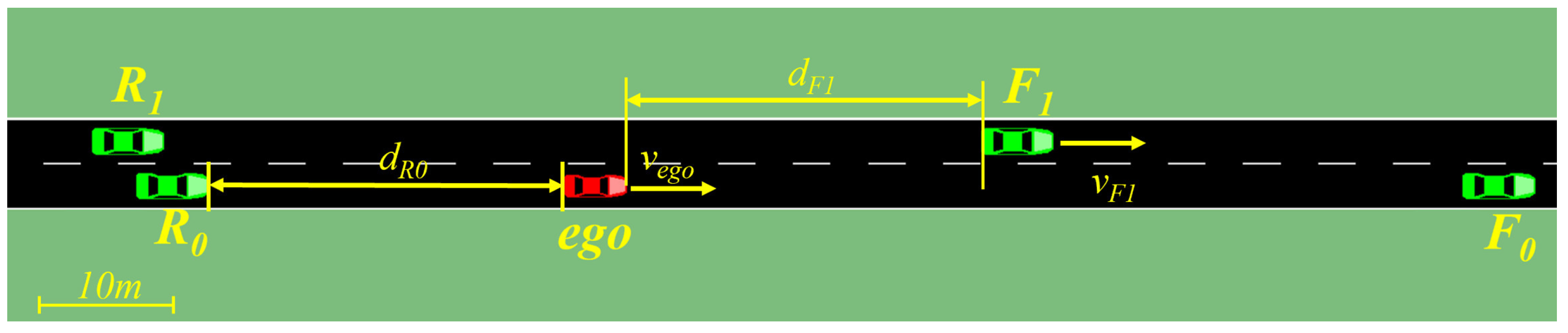The surrounding vehicles on the road have an initial speed of 8.33 m/s and a maximum speed of 16.67 m/s, and they use the IDM [16] model for longitudinal control and the SL2015 [35] model for lateral control. In this study, we trained with a traffic flow density of 15 veh/km. As shown in Figure 1, the red vehicle represents the ego vehicle, and the green vehicles represent other vehicles.

3.2. Environment State

In this paper, the state is characterized by ten variables: the distance $d_{F_0}$ between the ego vehicle and the vehicle in front, the distance $d_{R_0}$ between the ego vehicle and the vehicle behind, the distance $d_{F_1}$ between the ego vehicle and the vehicle in front on the target lane, and the distance $d_{R_1}$ between the ego vehicle and the vehicle behind on the target lane. Additionally, the speeds $v_{F_0}$, $v_{F_1}$, $v_{R_0}$, and $v_{R_1}$ of these four vehicles, as well as the speed $v_{\mathrm{ego}}$ and acceleration $a_{\mathrm{ego}}$ of the ego vehicle, are considered.

$$s=\{v_{F_1},d_{F_1},v_{R_1},d_{R_1},v_{F_0},d_{F_0},v_{R_0},d_{R_0},v_{ego},a_{ego}\},$$

(11)

3.3. Control Action

In this study, the continuous action of the control output is acceleration, and the discrete action is the lane-change decision. Vehicle dynamics and latency are not considered; hence, the vehicle instantaneously executes upon receiving an acceleration command or a lane-change decision. In training, the updates of the vehicle’s velocity, position, and lane-change decision occur at a time step of $0.1$ s, whereas in testing, the lane-change decision is output every 1 s. Moreover, accounting for the actual vehicle’s limits, the limit for continuous actions is defined as $[a_{min},a_{max}]=[-9.8,5.0]{\mathrm{m}/\mathrm{s}}^2$, where $a_{min}$ and $a_{max}$ represent the minimum and maximum accelerations, respectively.

The action space is defined as a tuple $A=(a_{\mathrm{continuous}},a_{\mathrm{discrete}})$, where $a_{\mathrm{continuous}}$ represents the continuous control of the vehicle’s acceleration, bounded by $a\in [a_{min},a_{max}]$. $a_{\mathrm{discrete}}$ is the discrete lane-change decision, where $a_{\mathrm{discrete}}=1$ indicates changing to another lane, and $a_{\mathrm{discrete}}=0$ signifies maintaining the current lane.

3.4. Reward

In the context of autonomous vehicle control, reward functions are designed to promote safe, efficient, and comfortable driving behavior. These functions are itemized as follows:

(1) This reward function aims to reduce meaningless lane change caused by the ego vehicle.

$$r_{lc}=\left\{\begin{array}{cc}-4,\hfill & \mathrm{if}{d}_{\mathrm{front}}<25\mathrm{m}\mathrm{and}\mathrm{lane}\mathrm{change}\mathrm{is}\mathrm{decided}\hfill \\ -20,\hfill & \mathrm{if}{d}_{\mathrm{front}}\ge 25\mathrm{m}\mathrm{and}\mathrm{lane}\mathrm{change}\mathrm{is}\mathrm{decided}\hfill \end{array}\right.$$

(12)

(2) $d_{\mathrm{safe}}$ represents the safe following distance from the vehicle ahead in the same lane, which is set to 25 m in this study. $v_{\mathrm{limit}}$ denotes the minimum speed limit for the lane when the distance to the vehicle ahead exceeds the safe distance.

$$r_{\mathrm{spd}}=\left\{\begin{array}{cc}0.1 \times |v_{\mathrm{ego}}-v_{\mathrm{limit}}|,\hfill & v_{\mathrm{ego}}\in [13.89\mathrm{m}/\mathrm{s},16.67\mathrm{m}/\mathrm{s}]\mathrm{and}{d}_f\ge d_{\mathrm{safe}}\hfill \\ -0.1 \times |v_{\mathrm{ego}}-v_{\mathrm{limit}}|,\hfill & v_{\mathrm{ego}}\notin [13.89\mathrm{m}/\mathrm{s},16.67\mathrm{m}/\mathrm{s}]\mathrm{and}{d}_f\ge d_{\mathrm{safe}}\hfill \end{array}\right.$$

(13)

(3) To facilitate the ego vehicle’s acquisition of car-following behavior and to mitigate the risk of collisions, we devised the following reward function predicated on the vehicle-to-vehicle distance metric:

$$r_{\mathrm{dis}}=\left\{\begin{array}{cc}-1·(d_{\mathrm{safe}}-min(d_{F0},d_{R0})),\hfill & \mathrm{if}{d}_{F0}\le d_{\mathrm{safe}}\mathrm{or}{d}_{R0}\le d_{\mathrm{safe}}\hfill \\ 0,\hfill & \mathrm{otherwise}\hfill \end{array}\right.$$

(14)

where $d_{R0}$ represents the distance to the rear vehicle in the same lane and $d_{F0}$ denotes the distance to the forward vehicle in the same lane.

(4) To instruct the ego vehicle to autonomously navigate lane change while mitigating collision occurrences, a penalty of $r_{\mathrm{collision}}=-200$ is incurred following each collision event.

(5) To reduce the jerk during the ego vehicle’s motion, we defined the following reward function:

$$r_{\mathrm{jerk}}=-0.005\times |a_t-a_{t-1}|$$

(15)

where $a_t$ represents the acceleration of the ego vehicle at the current time step and $a_{t-1}$ represents the acceleration of the ego vehicle at the previous time step.

(6) For safe reinforcement learning, we employ the TTC as a cost metric. The TTC is expressed as

$$TTC=\frac{v_{ego}-v_{other}}{d_{relative}}$$

(16)

where $v_{\mathrm{ego}}$ represents the velocity of the ego vehicle, $v_{\mathrm{other}}$ denotes the velocity of other vehicles, and $d_{\mathrm{relative}}$ indicates the relative distance between the ego vehicle and other vehicles. When the TTC between the ego vehicle and either the leading or following vehicle is less than 2.7 s but greater than 0, the cost is incremented by 1; if the TTC is equal to or greater than 2.7 s or the TTC is not calculable (due to no vehicle being present), the cost remains at 0.

For the PASAC algorithm, the total reward at each timestep is given by

$$r_{total}=r_{lc}+r_{spd}+r_{dis}+r_{jerk}+r_{collision}$$

(17)

For the PASAC-PIDLag algorithm, the total reward and cost at each timestep are given by

$$\begin{array}{cc}\hfill r_{\mathrm{total}}& =r_{\mathrm{lc}}+r_{\mathrm{spd}}+r_{\mathrm{dis}}+r_{\mathrm{jerk}}\hfill \\ \hfill \mathrm{Cos}\mathrm{t}& =\left\{\begin{array}{cc}\mathrm{Cos}\mathrm{t}+1\hfill & \mathrm{if}0<\mathrm{TTC}<2.7\mathrm{s}\hfill \\ \mathrm{Cos}\mathrm{t}\hfill & \mathrm{if}\mathrm{TTC}\ge 2.7\hfill \end{array}\right.\hfill \end{array}$$

(18)

We do not include collisions in the cost calculation because the safety policy derived from safe RL may sometimes approach the collision constraint too closely, potentially resulting in collisions.

4. Experiments and Results

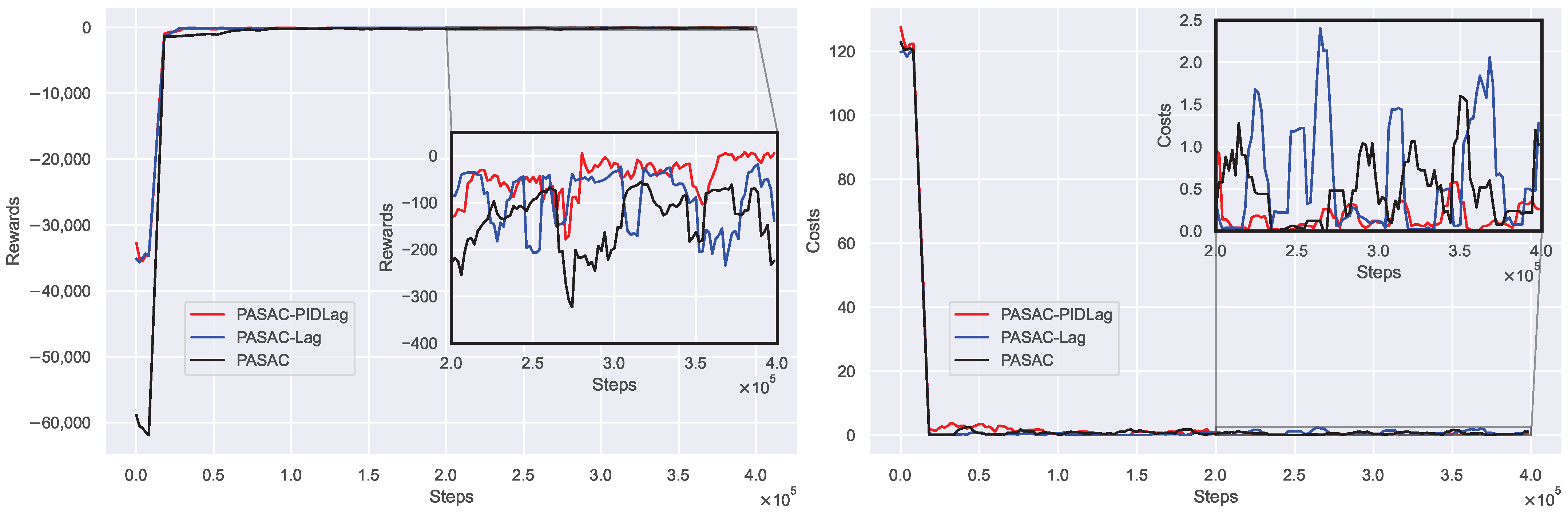
In this section, we present the training results under a traffic density of 15 veh/km. The PASAC-PIDLag algorithm outperforms the PASAC-Lag in terms of rewards and costs. The PASAC-Lag method is the traditional Lagrangian method that focuses solely on integral control. Therefore, we did not conduct tests on it. We analyzed both PASAC-PIDLag and PASAC algorithms under a traffic density of 15 veh/km. Additionally, we conducted a generalization analysis of these two algorithms under traffic densities of 10 veh/km and 18 veh/km.

4.1. Training

Our training setup consisted of an NVIDIA RTX 3060 GPU and an Intel i7-12700F CPU, with each training session running for approximately 5 h and covering 400,000 timesteps. The timestep interval was set at 0.1 s to better reflect real-world scenarios. Additionally, we initialized vehicles on the main road within a 50 m buffer zone at the start of each episode. The initial speed of the ego vehicle was set to 8.33 m/s. At the beginning of each episode, the lane for ego vehicle departure was randomly chosen from the two-lane road. During the training process, we evaluated ten episodes for each training episode, and we selected the best-performing policy as the model for subsequent testing.

The hyperparameter configurations for the PASAC-PIDLag, PASAC-Lag, and PASAC algorithms are listed in

Table 1. The hyperparameter values for the PASAC-PIDLag, PASAC-Lag, and the PASAC algorithms.

Hyperparameter	PASAC-PIDLag	PASAC-Lag	PASAC
Discount factor $\gamma$	0.99	0.99	0.99
Temperature parameter $\alpha$	0.2	0.2	0.2
The learning rate of the Actor network	0.0001	0.0001	0.0001
The learning rate of the Critic network	0.0003	0.0003	0.0003
Initial learning steps	10,000	10,000	10,000
The size of the batch	256	256	256
The size of the replay buffer	1,000,000	1,000,000	1,000,000
The soft update coefficient	0.005	0.005	0.005
The $K_p$ of the PID controller	0.000002	-	-
The $K_i$ of the PID controller	0.0000002	-	-
The $K_d$ of the PID controller	0.0000001	-	-
Tolerance of constraint violation	0	0	-
Initial Lagrange multiplier value	0.001	0.001	-
Initial value of Lagrangian multiplier	-	0.000002	-

. Figure 2 illustrates the training curves for these algorithms. From the training curves, it is evident that the PASAC-PIDLag algorithm demonstrates superior performance compared to both the PASAC-Lag and PASAC algorithms. The training curve of the PASAC-PIDLag algorithm outperforms that of the PASAC-Lag, as the incorporation of PID control in PASAC-PIDLag has successfully reduced the oscillation amplitudes of the cost, leading to more stable performance. Consequently, the PASAC-Lag algorithm was not considered for further testing.

4.2. Testing

In our experiments, we evaluated the performance of the trained policy over 400 episodes under a traffic density of 15 veh/km, encompassing approximately 300,000 timesteps. At the onset of each episode, the initial velocity of the ego vehicle was set to 8.33 m/s (equivalent to 30 km/h). Moreover, to assess the generalizability of our approach, we also conducted tests on the aforementioned strategy at traffic densities of 10 veh/km and 18 veh/km.

4.3. Comparison and Analysis

Based on the results obtained from the dataset of 400 test episodes, as shown in

Table 2. The results under a traffic flow density of 15 veh/km.

400 Episodes	PASAC-PIDLag	PASAC
Average reward	26.35	−53.13
Collision rate	0%	1%
Average speed (m/s)	14.36	14.04
Average jerk (m/s3)	0.315	0.415
Lane-change times	137	146

, it is evident that the PASAC-PIDLag algorithm outperformed the PASAC algorithm on multiple evaluation metrics. The PASAC-PIDLag algorithm exhibited a notably lower collision rate, indicating a safer driving policy adept at mitigating the risk of accidents more effectively. In addition, this algorithm necessitated fewer lane-change maneuvers, suggesting more stable and efficient driving behavior with the potential to diminish disruptive actions within the traffic flow. In terms of velocity, the PASAC-PIDLag algorithm achieved a higher average speed, a pivotal factor in enhancing the rate of transport. Moreover, the jerk metric was significantly reduced for the PASAC-PIDLag algorithm. Upon comprehensive consideration of these performance indicators, the PASAC-PIDLag algorithm surpassed the PASAC algorithm in terms of both optimality and safety.

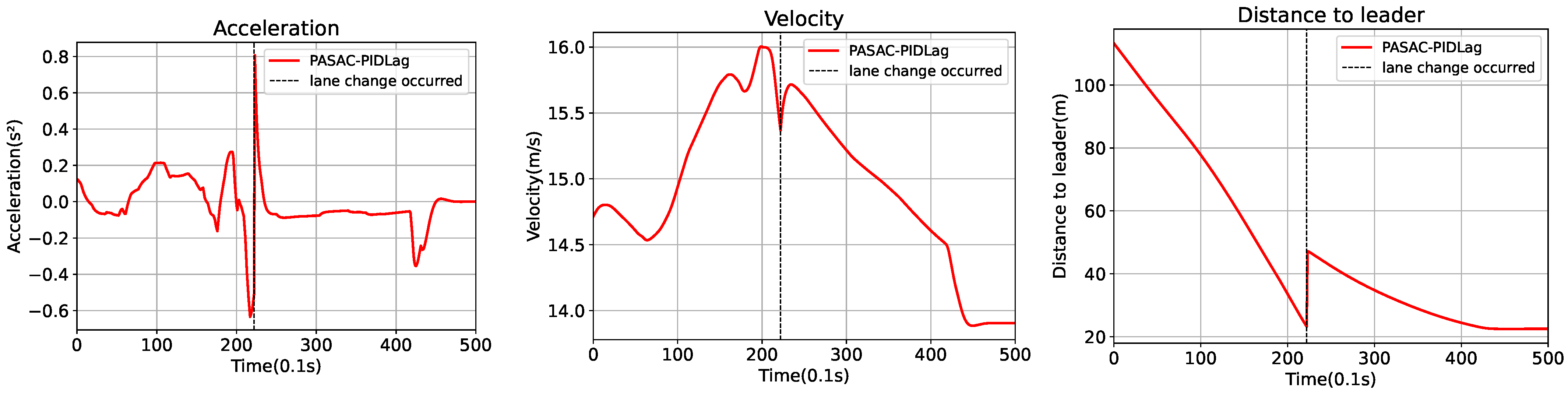
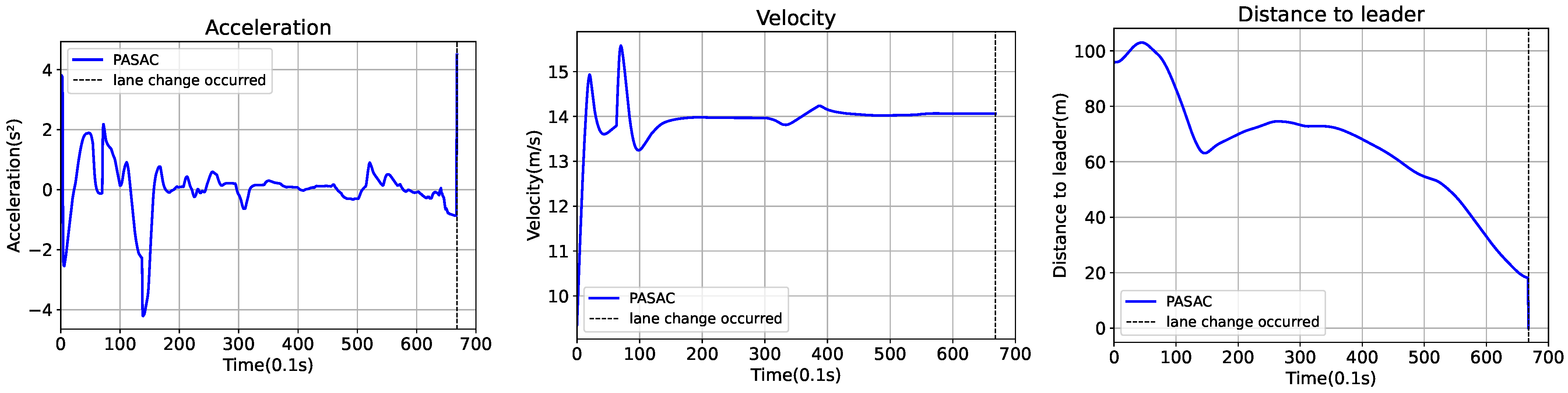
Figure 3 depicts an analysis of a lane-changing episode under the PASAC-PIDLag algorithm. Subsequent to this lane-change event, there was an immediate and discernible change in the distance to the preceding vehicle, indicative of the completion of the lane change. The graph detailing relative distance demonstrates that the vehicle initiated the lane-change maneuver when it was at a safe following distance of approximately 25 m. Moreover, the velocity graph depicts a modest escalation in the ego vehicle’s speed following the lane change, which was shortly followed by a decrease. 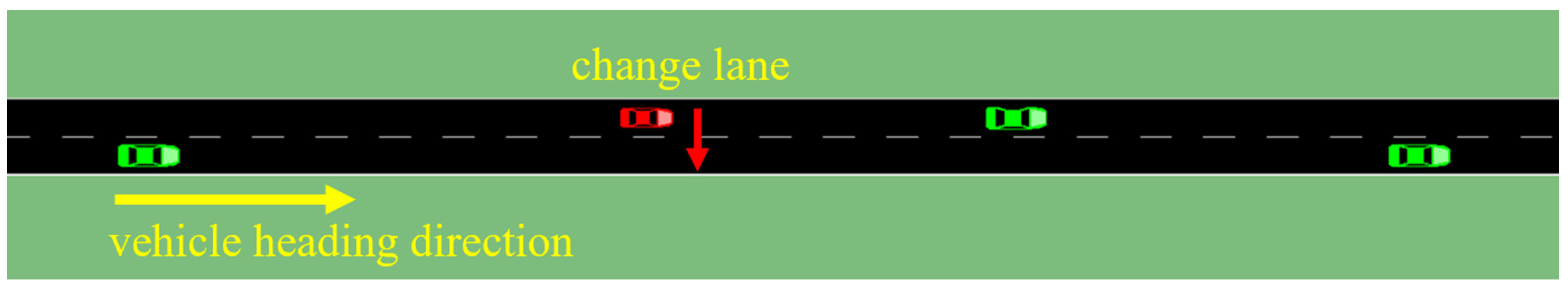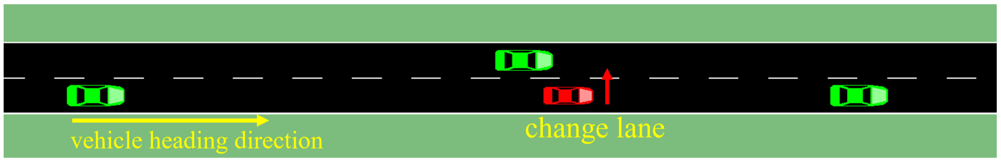Figure 4 presents the SUMO scene of the successful lane-change maneuver executed by the PASAC-PIDLag algorithm.

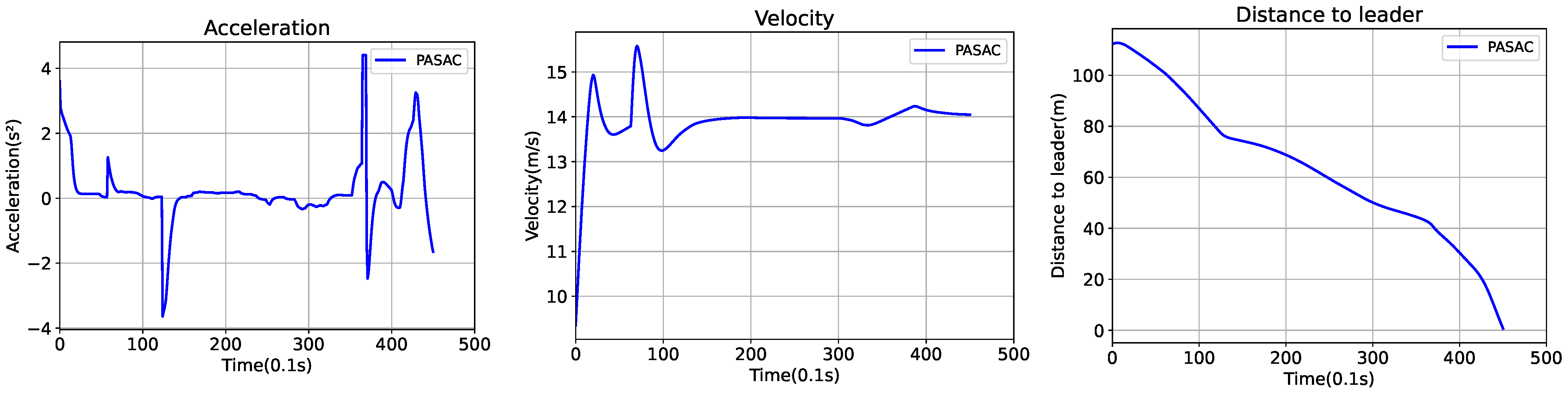
Figure 5 depicts an episode of collision occurrence within the PASAC algorithm framework, in which the ego vehicle collided after executing a lane change. The data presented in the figure reveal that the ego vehicle was steadily closing in on the vehicle ahead until the following distance diminished to 19 m, which triggered a decision to change lanes. At this juncture, the presence of another vehicle in the target lane led to a collision. Figure 6 displays the instance of a lane-change maneuver resulting in a collision in SUMO, as directed by the PASAC algorithm.

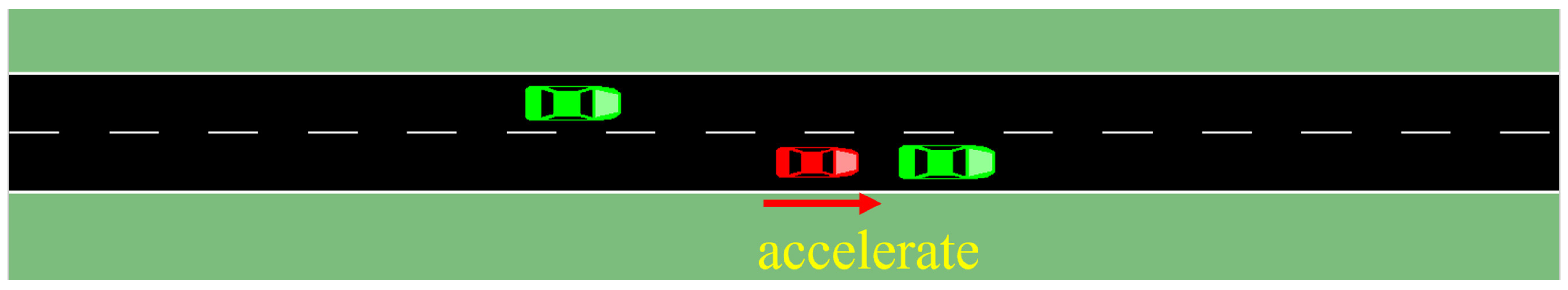
Figure 7 illustrates another scenario in which a collision occurred under the PASAC algorithm, where the ego vehicle collided during the car-following process. The data and the figure show that due to the presence of a vehicle in the adjacent lane, the ego vehicle was unable to change lanes, resulting in a collision during car following. Figure 8 presents an example of a collision involving an ego vehicle trained using the PASAC algorithm in a car-following scenario in SUMO.

A comparison of lane-changing decisions between the PASAC and PASAC-PIDLag algorithms demonstrated that the strategy derived from the PASAC algorithm was sometimes incapable of effectively balancing the decision related to lane changing and car following under certain conditions.

4.4. Generalization Analysis

To evaluate the generalizability of the proposed algorithm, we first conducted tests under a traffic density of 10 veh/km, and the results are presented in

Table 3. The generalization results under a traffic flow density of 10 veh/km.

400 Episodes	PASAC-PIDLag	PASAC
Average reward	−24.98	−71.32
Collision rate	0%	0%
Average speed (m/s)	14.51	14.06
Average jerk (m/s3)	0.290	0.329
Lane-change times	82	78

. The data presented in Table 3 reveal that at such a reduced traffic density, both algorithms demonstrated the ability to maintain a collision rate of zero. Notwithstanding this equivalence in safety, the PASAC-PIDLag algorithm surpassed its counterpart, PASAC, by securing a greater average reward, attaining a higher mean velocity, and exhibiting a lower average jerk. These findings imply that the PASAC-PIDLag algorithm not only meets safety benchmarks but also excels in performance, offering an enhanced level of optimality over the PASAC algorithm.

Our final series of tests were conducted at a traffic flow density of 18 veh/km. The results outlined in

Table 4. The generalization results under a traffic flow density of 18 veh/km.

400 Episodes	PASAC-PIDLag	PASAC
Average reward	−136.07	−150.25
Collision rate	0.25%	2.25%
Average speed (m/s)	14.17	13.98
Average jerk (m/s3)	0.290	0.329
Lane-change times	226	164

reveal that at this higher traffic density, the collision rate of the PASAC-PIDLag algorithm remained lower than that of the PASAC algorithm. Furthermore, the PASAC-PIDLag algorithm demonstrated its superiority across all measured metrics, including average reward, average speed, and average jerk.

5. Conclusions

In this paper, we introduced PASAC-PIDLag, a safe hybrid-action reinforcement learning algorithm specifically applied to the scenario of autonomous lane change. This method represents a novel approach that aims to enhance both safety and optimality in the application of reinforcement learning in the autonomous driving domain. We compared it with its unsafe version, PASAC. Both algorithms were trained and tested under a traffic flow density of 0.15 veh/km and underwent generalization tests at densities of 0.10 veh/km and 0.18 veh/km. The results indicated that at a traffic density of 15 veh/km, the strategy trained by the PASAC-PIDLag algorithm managed to maintain zero collisions, while the collision rate for the PASAC algorithm was observed to be 1%. The PASAC algorithm was observed to encounter two types of collisions at a density of 15 veh/km. The reward structure in this study involves both lane changing and car following, which may lead to collisions arising from unsuccessful lane-changing or car-following maneuvers.

Both algorithms achieved zero collisions at a lower traffic density of 10 veh/km. At a higher traffic density of 18 veh/km, the collision rate of the PASAC-PIDLag algorithm was lower than that of the PASAC algorithm. Across the three traffic densities, the PASAC-PIDLag algorithm consistently achieved higher average speeds, lower average jerks, and greater average rewards. Overall, the PASAC-PIDLag algorithm showed superior performance with respect to safety and optimality.

In future work, we aim to further the application of safe reinforcement learning-based control in actual vehicles. Applying reinforcement learning to real vehicles presents numerous challenges, particularly regarding varying road conditions. In subsequent efforts, we plan to utilize driving simulation software to create road scenarios with obstacles such as construction zones, potholes, and lane congestion. Training within these simulated environments will address the challenge of adapting to diverse road conditions. Additionally, we will employ meta-reinforcement learning to rapidly adapt to different road conditions.