Highly Self-Adaptive Path-Planning Method for Unmanned Ground Vehicle Based on Transformer Encoder Feature Extraction and Incremental Reinforcement Learning

Abstract

Path planning is an indispensable component in guiding unmanned ground vehicles (UGVs) from their initial positions to designated destinations, aiming to determine trajectories that are either optimal or near-optimal. While conventional path-planning techniques have been employed for this purpose, planners utilizing reinforcement learning (RL) exhibit superior adaptability within exceedingly complex and dynamic environments. Nevertheless, existing RL-based path planners encounter several shortcomings, notably, redundant map representations, inadequate feature extraction, and limited adaptiveness across diverse environments. In response to these challenges, this paper proposes an innovative and highly self-adaptive path-planning approach based on Transformer encoder feature extraction coupled with incremental reinforcement learning (IRL). Initially, an autoencoder is utilized to compress redundant map representations, providing the planner with sufficient environmental data while minimizing dimensional complexity. Subsequently, the Transformer encoder, renowned for its capacity to analyze global long-range dependencies, is employed to capture intricate correlations among UGV statuses at continuous intervals. Finally, IRL is harnessed to enhance the path planner’s generalization capabilities, particularly when the trained agent is deployed in environments distinct from its training counterparts. Our empirical findings demonstrate that the proposed method outperforms traditional uniform-sampling-based approaches in terms of execution time, path length, and trajectory smoothness. Furthermore, it exhibits a fivefold increase in adaptivity compared to conventional transfer-learning-based fine-tuning methodologies.

1. Introduction

Unmanned ground vehicles (UGVs) have emerged as a significant technological advancement with far-reaching applications across various fields. Their ability to operate without human presence in potentially hazardous or challenging environments makes them invaluable assets [1,2,3]. In the military domain, UGVs contribute to safeguarding personnel by undertaking tasks like bomb disposal and reconnaissance in hostile territories. Additionally, their deployment in risky industrial settings, such as hazardous material handling or mining operations, minimizes human exposure to potential dangers. Furthermore, UGVs play an increasingly crucial role in civilian sectors, including agriculture, where they automate tasks like crop monitoring and precision spraying, leading to enhanced efficiency and resource optimization. Therefore, the growing sophistication and versatility of UGVs underscore their importance as transformative tools for improving safety, efficiency, and productivity across diverse domains [4].

The success of UGVs in achieving their designated tasks hinges critically on the efficacy of path-planning algorithms, which play a pivotal role in determining the optimal or near-optimal trajectory for a UGV to navigate from its starting point to its destination [5,6]. By factoring in environmental constraints, obstacles, and potential hazards, path-planning algorithms enable UGVs to operate safely and efficiently. In dynamic environments, path-planning algorithms become even more crucial, as they must adapt to unforeseen changes in real time, ensuring the UGV avoids collisions and navigates safely. The continued development and refinement of path-planning algorithms are therefore paramount for ensuring the safe, reliable, and successful operation of UGVs across various applications [7].

Path-planning algorithms for UGVs can be mainly divided into traditional classical algorithms [8,9] and learning-based methods [10,11,12]. Traditional classic algorithms generally obtain the optimized path in complex environments through a hierarchical architecture incorporating a global planner and a local planner [13]. The global planner generates the global path from the starting point to the target point in the entire environment considering the map, obstacles, and other environmental information at a global scale. Then, the local planner uses the global path as a reference and adjusts the path to adapt to dynamic obstacles or other unexpected situations. Classic global path planners include the Dijkstra algorithm [14], Prim algorithm [15], visible graph algorithm [16], probabilistic roadmap algorithm [17], etc., while local path planners include the dynamic window method [18] and time elastic band algorithm [19], etc. Although traditional path planners have a good theoretical foundation and application robustness, they cannot demonstrate good adaptability in extremely complex and dynamic environments due to high-dimensional nonlinear and complicated constraints. In order to solve the above problems, learning-based path-planning algorithms [20], especially reinforcement learning (RL)-based methods [21], have received increasing attention in recent years.

Path planners based on RL can improve their strategies through continuous interaction with the environment, thereby obtaining an optimized policy. This kind of method can effectively handle high-dimensional-state spaces and is suitable for application in dynamic environments that require the consideration of complex perceptual information, surpassing traditional classical algorithms by a large margin. RL-based path planners generally first perform a mathematical representation of the environment, and then use feature-extraction technology to extract features that are important to path planning from information such as environmental representation or the status of the UGV to form a state vector. Finally, the planner will establish a neural network to implement end-to-end mapping from the state vector to the control instructions. However, existing RL-based path planners are confronted with three drawbacks in terms of map representation, feature extraction, and adaptive capability.

Regarding map representation, prevalent methods employed by existing path planners entail utilizing either a global occupancy map or the direct input of the original camera or 3D lidar points from the immediate environment. For instance, Chen et al. employed a convolutional neural network (CNN) trained on an egocentric local occupancy map to predict optimal steering actions for a robotic system, demonstrating the feasibility of deploying a map-based end-to-end navigation model onto real-world robotic platforms [22]. Similarly, Wang et al. introduced an off-road path-planning approach based on deep RL, training the agent within a low-dimensional simulator constructed using occupancy maps [23]. Furthermore, Fan et al. proposed a hierarchical RL-based path planner for exploring unknown spaces, utilizing lidar readings alongside iteratively generated occupancy maps as observations for the RL agent [24]. However, while employing original occupancy maps or sensor observation data as inputs for UGV path planning facilitates the preservation of environmental information to a large extent, it also presents challenges. The high dimensionality of such data, particularly in the case of high-resolution maps or dense sensor data, can markedly augment the computational complexity of subsequent path-planning algorithms. Consequently, this may compromise the efficiency and real-time performance of the planning system, which are crucial for ensuring safe and dependable autonomous navigation within dynamic environments.

In terms of feature extraction, the majority of existing RL-based path-planning methodologies employ convolutional neural networks (CNNs) or fully connected networks (FCNs) as foundational architectures for information extraction [25,26]. This preference is rooted in the remarkable efficacy of CNNs in image processing tasks, rendering them well suited for handling image-like map representations, while FCNs are favored for their versatility and simplicity. For instance, Sartori et al. leveraged a CNN to extract salient features from a top-down environmental image, encompassing obstacle distributions as well as the locations of starting and goal points [27]. Similarly, Jin et al. introduced a pyramid path-planning network, amalgamating a CNN with a feature-pooling pyramid structure to extract multiscale features from various hierarchical levels, thereby generating a local feature representation enriched with semantic information [28]. Additionally, Qureshi et al. employed an FCN to amalgamate environmental features such as raw point clouds obtained from depth sensors, alongside a robot’s initial and target configurations [29]. However, notwithstanding their proficiency in local feature extraction, CNNs and FCNs encounter challenges in capturing long-range dependencies, a pivotal aspect for effective path planning.

As for adaptive capability, the prevailing paradigm among RL-based path planners is predicated upon the assumption that the deployed agent will encounter environments possessing similarities to those present during training phases. For instance, Bae et al. conducted training and testing of a deep Q-learning RL agent on congruent grid-like occupancy maps [30]. Similarly, Wang et al. introduced a pioneering path-planning methodology for multi-agent systems, integrating flocking control and RL, wherein both training and testing simulations were conducted within the same environments developed utilizing Visual Studio Community software and the Unity3D engine [31]. Furthermore, Huang, R. et al. put forward an RL-based path planner for a continuous dynamic simulation environment, where the obstacles were all circle-like in the training and testing environments [32]. While this presumption of congruent obstacle features and distributions across training and testing settings facilitates, to some extent, the applicability of RL-based path planners, such scenarios remain uncommon in real-world applications. It is more typical for application scenarios to exhibit significant disparities from training environments, thereby diminishing the performance of trained RL agents when faced with unseen environments. Consequently, there is a pressing need for a highly self-adaptive path-planning framework to augment the generalization capabilities of trained RL agents.

In order to overcome the above three existing drawbacks, this paper proposes a novel RL-based path planner with highly self-adaptive capability combining a Transformer encoder block and incremental reinforcement learning (IRL) using compressed map representation as the input. The contributions of this study include the following three aspects.

• Firstly, the original 2D map is compressed to a 1D feature vector using an Autoencoder to lighten the computational burden of following the RL path planner. The compressed 1D feature vector can achieve a highly accurate reconstruction of the original 2D map, thus ensuring abundant and ample information is obtained while the input dimension is greatly reduced.
• Secondly, the Transformer encoder block, which has global long-range dependency analysis capability, is adopted to capture the highly intertwined correlation between UGV status at continuous instances. The results show that the Transformer encoder demonstrates better optimality than a traditional CNN or FCN thanks to its strong feature-extraction capability.
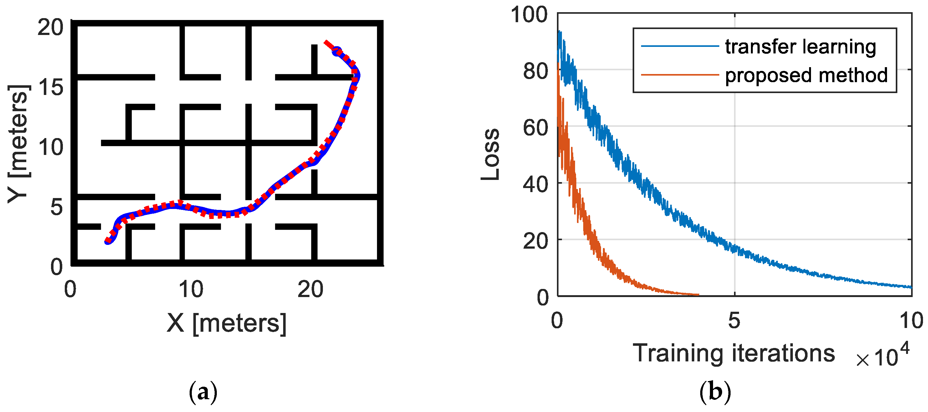
• Thirdly, incremental reinforcement learning (IRL) is adopted to improve the path planner’s generalization ability when the trained agent is deployed in totally different environments to the training environments. The results show that ICR can achieve 5× faster adaptivity than traditional transfer-learning-based fine-tuning methods.

The remainder of this paper is organized as follows. Section 2 will detail the general framework of the proposed path planner, together with the relevant theoretical foundations involved. Section 3 will validate the proposed method in various simulation environments and compare it with the uniform-sampling-based and transfer learning of fine-tuning methods. Section 4 will conclude the whole paper and point out possible future research directions.

2. Methodology

The general framework of the proposed path-planning method is shown in Figure 1. Firstly, the RL agent prepares input information for the path-planning decision. The inputs include three aspects, namely the compressed map representation, the target point, and the UGV’s status. The compressed map representation is a latent representation of the original 2D map given by the autoencoder, which will be discussed in detail in Section 2.1. Because the first two items are invariant during the whole path-planning process, they are directly fed to the IRL module. The UGV status, including its x-coordinate, y-coordinate, and orientation, will change as the UGV moves; therefore, status information from a past time window with a length of n will be collected and fed into the Transformer encoder. Then, four consecutive Transformer encoder layers will process the UGV status information and fully exploit the temporal correlation of the UGV’s movements. The Transformer encoder layer will be introduced in Section 2.2. Finally, the output of the Transformer, together with the two direct inputs, will be processed by the IRL module, where incremental learning will be incorporated to improve the agent’s generalization ability in different environments. The process of IRL will be elaborated upon in Section 2.3.

It is imperative to underscore that classical-sampling-based planners, such as rapidly exploring random trees (RRT), RRT*, or bidirectional-RRT, typically rely on generating samples uniformly distributed across a designated state space. However, these planners commonly confine the UGV within a limited portion of the state space. Consequently, the uniform sampling strategy leads to the exploration of numerous states that have a negligible influence on the final path. This inefficiency significantly hampers the planning process, particularly within state spaces characterized by high dimensionality and environments featuring narrow passages. To address this challenge, the proposed method endeavors to reduce the sampling space from the entirety of the state space to an optimal subset, guided by the path-planning outcomes derived from RRT or RRT*. This strategic adjustment notably enhances the efficiency of the path-planning process. For further elaboration, please refer to Section 3.

2.1. Autoencoder for Environment Representation

An autoencoder is a type of artificial neural network trained to compress and reconstruct its input data [33]. In simpler terms, it aims to learn a compressed representation of the input while still being able to accurately recreate the original data from this compressed version. An autoencoder consists of two main parts, namely an encoder and a decoder. The encoder part takes the input data and compresses it into a lower-dimensional representation, often called the latent space. This compressed version captures the essential features of the input. The decoder part receives the latent space representation and tries to reconstruct the original input data from it. The general framework of the autoencoder is shown in Figure 2.

Let us denote the encoder network and the decoder network as h = f(x) and y = g(h), where x, h, and y represent the input, latent representation, and output, respectively. The encoder and decoder networks can take arbitrary networks, including the FCN, CNN, recurrent neural network (RNN), etc. [34]. Because here, we want to compress the two-dimensional environment map into the latent space, the CNN is selected as the encoder network considering its superior capability in processing image-like two-dimensional inputs.

Within a convolutional layer, a learnable filter, usually referred to as a kernel, is applied to the map, followed by processing with an activation function. The mathematical formula of the CNN layer can be expressed as [35]

$$x_j^l=\sum _{i\in M_j}{x}_i^{l-1}\ast k_{ij}^l+b_i^l$$

(1)

where $x_j^l$ represents the jth feature map of the ith convolutional layer; M_j represents the collection of input feature maps; * denotes the convolutional operation; and b represents the additional bias added to the output graph.

After being processed by the CNN layer, the obtained feature map is usually smaller than the original input, mainly due to the stride and convolutional operation. Because the autoencoder tries to reconstruct the original input, the decoder network needs to upsample the feature map output by the encoder network to the same size as the original input. Therefore, transposed convolution, also known as fractionally strided convolution, is introduced into the decoder network. It is essentially the reverse operation of convolution and allows the network to learn to upsample the information and generate a larger image. It achieves this by introducing learnable filters and performing similar element-wise multiplication and summation. Details of the mathematical operation of transposed convolution can be found in Ref. [36].

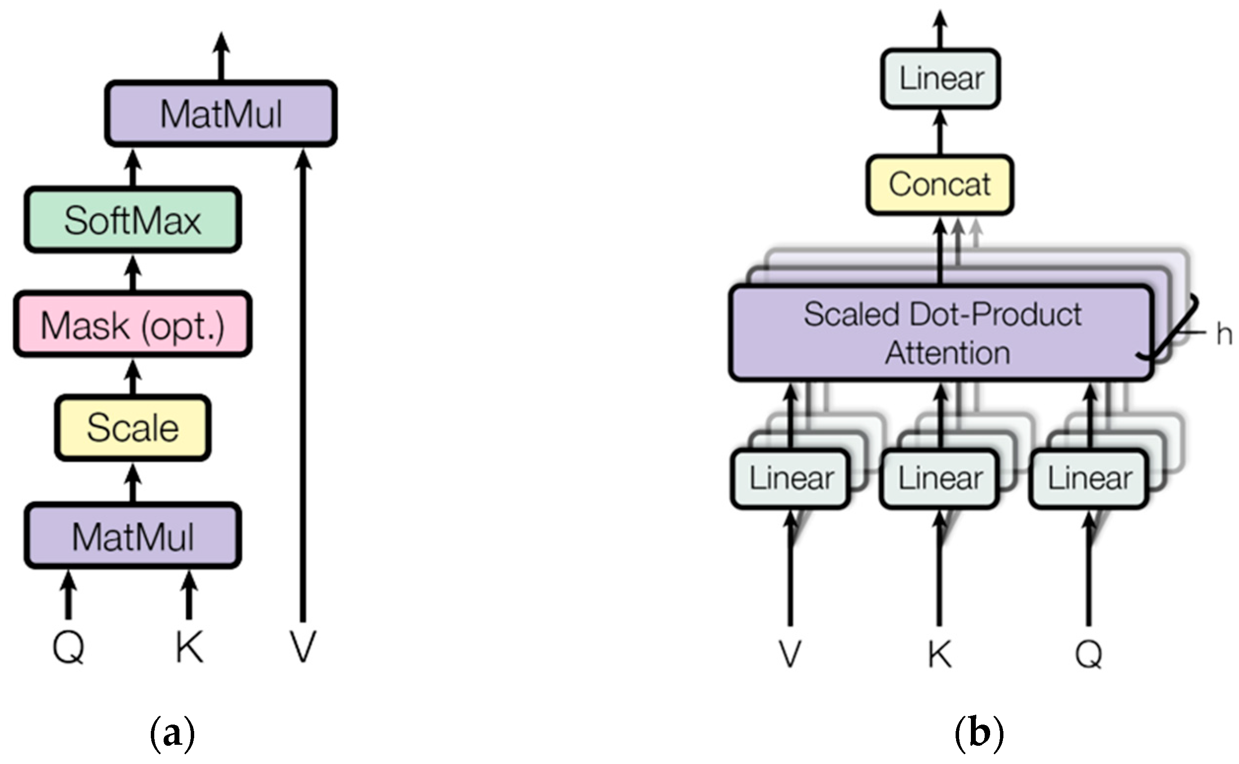
2.2. Transformer Encoder Layer

The Transformer encoder, a core component in many deep learning architectures, utilizes a stacked structure of identical layers. Each layer is composed of two sub-layers: a multi-head attention mechanism and a fully connected feed-forward network [37]. The multi-head attention allows the model to attend to relevant parts of the input sequence, while the feed-forward network introduces non-linearity for complex feature extraction [38]. Residual connections and layer normalization are implemented around each sub-layer to address vanishing gradients and accelerate training, respectively. This design enables the encoder to effectively capture long-range dependencies within the input data.

At the heart of the Transformer encoder lies the multi-head attention mechanism, as shown in Figure 3. This mechanism splits the model’s representation into multiple heads, each acting as a subspace that allows the model to attend to different aspects of the input information. The outputs from these heads are then concatenated, enabling the network to capture a richer and more nuanced understanding of the features within the data. Here scaled dot-product attention is adopted and the computational formulas are shown in Equations (2)–(5).

$$\left\{\begin{array}{c}Q=W^{Q}X\\ K=W^{K}X\\ V=W^{V}X\end{array}\right.$$

(2)

$$Attention\left(Q,K,V\right)=softmax\left(\frac{Q{K}^T}{\sqrt{d}}\right)V$$

(3)

$$H_i=Attention\left(Q{W}_i^Q,K{W}_i^K,V{W}_i^v\right)$$

(4)

$$MultiHead\left(Q,K,V\right)=\left[H_1,\dots ,H_h\right]W_o$$

(5)

Here, the query matrix Q, key matrix K, and value matrix V are generated by transforming the feature vector matrix X; W^Q, W^K, and W^V are all linear transformation matrices; d is the scaling factor; $W_i^Q$, $W_i^K$, and $W_i^v$ are the transformation matrices projecting Q, K, and V into the ith subspace, where i ranges from 1 to h, and h is the total number of subspaces; H_i represents the single-head attention values in the ith subspace; and $W_i^v$ is the transformation matrix used to concatenate the attention values from all subspaces.

2.3. Incremental Reinforcement Learning

This paper proposes an RL path-planning model based on incremental learning, namely the incremental collaborative learning knowledge model (ICLKM) [39]. For the RL part, we adopt the advanced soft actor–critic (SAC) algorithm.

The SAC algorithm distinguishes itself from other deep RL approaches by incorporating the concept of entropy, a measure of randomness in probability distributions [40]. In the context of SAC, entropy reflects the level of stochasticity, unpredictability, or variation within an agent’s actions. Higher entropy values signify increased action randomness, resulting in richer exploration of potential actions. This entropy injection encourages policy exploration within the state space, mitigating the risk of becoming trapped in local optima. By enabling the exploration of diverse solution pathways, entropy ultimately enhances the robustness of the final learned policy. The specific mathematical formula for calculating entropy is

$$H\left(\pi \left(\cdot ∣s\right)\right)=E_a\left[-\mathit{log}\pi \left(\cdot ∣s\right)\right]$$

(6)

In the realm of general RL algorithms, the objective centers on acquiring a strategy that maximizes the total accumulated reward received by the agent throughout its interactions with the environment [41]. In simpler terms, the goal is to learn a course of action that yields the greatest overall benefit for the agent, namely

$${\pi }^{\ast }=\underset{\pi }{\mathit{argmax}}{E}_{\left(s_t,a_t\right)\sim {\rho }_{\pi }}\left[\sum _{t}r\left(s_t,a_t\right)\right]$$

(7)

For the SAC algorithm, in addition to the above general objectives, it is also required that the strategy has the maximum entropy at each output action:

$${\pi }^{\ast }=\mathit{arg}\underset{\pi }{\mathit{max}}{E}_{\left(s_t,a_t\right)\sim {\rho }_{\pi }}\left[\sum _t\underset{\mathit{reward}}{\underbrace{r\left(s_t,a_t\right)}}+\underset{\mathit{entropy}}{\underbrace{\alpha H\left(\pi \left(\cdot ∣s_t\right)\right)}}\right]$$

(8)

Its purpose is to ensure the randomness of the strategy, making each output action as dispersed as possible, and improving the exploration ability of the intelligent agent. The core idea of maximum entropy in motion planning tasks is to sample as many useful trajectories as possible.

In the SAC algorithm, the state value function $V_{\mathit{soft}}^{\pi }\left(s\right)$ can be expressed as

$$V_{\mathit{soft}}^{\pi }\left(s\right)=E_{\left(s_t,a_t\right)\sim {\rho }_{\pi }}\left[{\sum }_{t=0}^{\infty }{\gamma }^t\left(r\left(s_t,a_t\right)+\right.\right.\left.\alpha H\left(\pi \left(\cdot ∣s_t\right)\right)\right)|s_0=s]$$

(9)

The action value function $Q_{\mathit{soft}}^{\pi }\left(s,a\right)$ can be expressed as

$$Q_{\mathit{soft}}^{\pi }\left(s,a\right)=E_{\left(s_t,a_t\right)\sim {\rho }_{\pi }}[\sum _{t=0}^{\infty }{\gamma }^{t}r\left(s_t,a_t\right)\left.+\alpha {\sum }_{t=0}^{\infty }{\gamma }^{t}H\left(\pi \left(\cdot ∣s_t\right)\right)∣s_0=s,a_0=a\right]$$

(10)

The SAC algorithm employs a unique network architecture consisting of one actor network and four critic networks. Two of the critics estimate the state-value function V(s), with corresponding target networks V_target(s) used for stabilization during training. The remaining two critics focus on the action value function Q(s, a). Notably, the actor network and both Q-networks are synchronously updated using their respective parameters, while their target counterpart needs to be fixed for a period of time before synchronizing the latest parameters with the V(s) network. During training, the experience replay pool D provides samples, and exploration noise ε drawn from a standard normal distribution is added to the actions. The loss function for the Q(s, a) is then defined as

$$J_Q\left(\theta \right)=E_{\left(s_t,a_t,s_{t+1}\right)\sim D}{[\frac{1}{2}{Q}_{\theta }\left(s_t,a_t\right)-(r\left(s_t,a_t\right)+\gamma V_{\overline{\theta }}\left(s_{t+1}\right))]}^2$$

(11)

The loss function of the actor network is

$$J_{\pi }\left(\varphi \right)=E_{s_t\sim D,a_t\sim {\pi }_{\varphi }}\left[\alpha \mathit{log}{\pi }_{\varphi }\left(a_t∣s_t\right)-\right.\left.Q_{\theta }\left(s_t,a_t\right)\right]$$

(12)

The reparameterization technique was introduced in the process of updating the actor network, which means that

$$a_t=f_{\varphi }\left({\epsilon }_t;s_t\right)=f_{\varphi }^{\mu }\left(s_t\right)+{\epsilon }_t\odot f_{\varphi }^{\sigma }\left(s_t\right)$$

(13)

Considering the practical applications, it is necessary to limit the output to a certain range, so a flattening tanh function needs to be added to limit the final output to (−1, 1):

$$a_t=\mathit{tanh}\left(a_t\right)$$

(14)

In the setting of incremental learning in path planning [42], the model will first learn from the sample training set D₀ to obtain a high-performance model M₀. When new environmental samples appear, the already trained model will be incrementally learned on the gradually emerging sample dataset D_t, and the entire model will be continuously updated to obtain M_t. To equip SAC with incremental learning capability, The SAC agent adopts a dual network structure of $M_{t^{\prime }}$ and M_t. When the model is learning from D_t, the first network $M_{t^{\prime }}$ uses knowledge distillation to approximate the current learnt path-planning model M_t−1, helping the model retain learned knowledge and reduce the forgetting of old knowledge when learning new knowledge. Then, the second network M_t learns new data, takes the output of the first network as the learning objective, and performs consistency loss on the outputs of the two networks at each training step, enabling the path-planning model to effectively learn new knowledge. Finally, the first network $M_{t^{\prime }}$ and the second network M_t learn together. $M_{t^{\prime }}$ uses mean squared error (MSE) loss, consistency loss, and distillation loss to update the internal parameters through backpropagation. M_t adopts a knowledge collaboration strategy to update the internal parameters to generate a more adaptive model for path planning.

In the proposed dual network structure, the first network model $M_{t^{\prime }}$ adopts the knowledge distillation method [43]. The distillation loss L_kd only relies on the previous model M_t−1. It considers the MSE loss calculated between the outputs of M_t−1 and $M_{t^{\prime }}$. Distillation loss L_kd is defined as

$$L_{kd}=\frac{1}{n}{\sum }_{i=1}^n{[{\hat{\tau }}_i\left(x\right)-{\tau }_i(x\left)\right]}^2$$

(15)

where n is the dimension of the outputs, and ${\hat{\tau }}_i\left(x\right)$ and ${\tau }_i\left(x\right)$ represent the outputs of $M_{t^{\prime }}$ and M_t−1, respectively.

When learning from D_t, the output of the second network model M_t using the new dataset D_t as the input will be adopted as the learning objective of the first network model $M_{t^{\prime }}$. By continuously maintaining consistency between the two networks, the path-planning model can effectively learn new knowledge from new data.

Before training, both the first network model $M_{t^{\prime }}$ and the second network model M_t use the previous model M_t−1 as the pretrained model for initialization. The consistency loss L_con of the two networks is

$$L_{con}=\frac{1}{n}{\sum }_{i=1}^n{[{\hat{\tau }}_i\left(x\right)-{\tau }_i^{\ast }(x\left)\right]}^2$$

(16)

where ${\tau }_i^{*}\left(x\right)$ represents the output of M_t.

In each step, the first network model $M_{t^{\prime }}$ is trained in a supervised manner by calculating the MSE loss L_mse:

$$L_{mse}=\frac{1}{n}{\sum }_{i=1}^n{[{\hat{\tau }}_i\left(x\right)-{\tau }_i^{gt}(x\left)\right]}^2$$

(17)

where ${\tau }_i^{gt}\left(x\right)$ represents the ground truth target point of the path-planning algorithm.

Therefore, $M_{t^{\prime }}$ updates the weights based on the MSE loss L_mse, distillation loss L_kd, and consistency loss L_con between the two networks, and updates the weights of the model $M_{t^{\prime }}$ through backpropagation of the loss function. The complete loss function L_all for $M_{t^{\prime }}$ is

$$L_{all}=L_{mse}+\lambda L_{kd}+\beta L_{con}$$

(18)

The weights of the network loss function are balanced by $\lambda$ and $\beta$. At the same time, the weight of the second network M_t is frozen, and the weight of the network model M_t is updated through a knowledge collaboration strategy to generate a more adaptive model, that is, the process of updating the weight of M_t using the exponential moving average of the weights in $M_{t^{\prime }}$:

$${\theta }_t^j=\alpha {\theta }_t^{j-1}+\left(1-\alpha \right){\theta }_{t^{\prime }}^j$$

(19)

where ${\theta }_t^j$ and ${\theta }_{t^{\prime }}^j$ represent the weights of the networks M_t and $M_{t^{\prime }}$, respectively, and $\alpha$ is the smoothing coefficient hyperparameter. The parameters are updated at each training step j.

Both the learnt network models, $M_{t^{\prime }}$ and M_t, can be used for path planning. However, compared to the first network model $M_{t^{\prime }}$, the second network model M_t uses a knowledge collaboration algorithm to make parameter updates more robust and reflect the learning state of the first network $M_{t^{\prime }}$, resulting in better prediction performance. Therefore, the network model M_t is used as the final model for path planning.

3. Validation

In this section, we will first introduce the simulation setup information, including the hardware configurations and the training/testing datasets that were used to train and evaluate the agent. Then, the effectiveness of the compressed map representation will be validated, especially its reconstruction capability. Afterwards, a comparison between the proposed Transformer encoder and other commonly used networks will be conducted to highlight the superiority of using the Transformer to extract features. Finally, the proposed method will be compared with traditional uniform path-planning samplers, and its fast adaptability to different environments will be highlighted.

3.1. Simulation Setup

Simulations were conducted on a computer with an Intel i9-11980HK CPU and an Nvidia RTX 3080Ti graphics card. To ensure the diversity of the training dataset so that the trained model could have better generalization ability, 200 maze map environments were generated. The size of maze maps was 10 m × 10 m, and the resolution and wall thickness were both 0.4 m. For each generated map, 2000 demonstration paths were generated by the RRT* algorithm. The generated RRT* paths were fed to the path-planning network as the training targets. Figure 4 shows four representative generated maps and the RRT* demonstration paths.

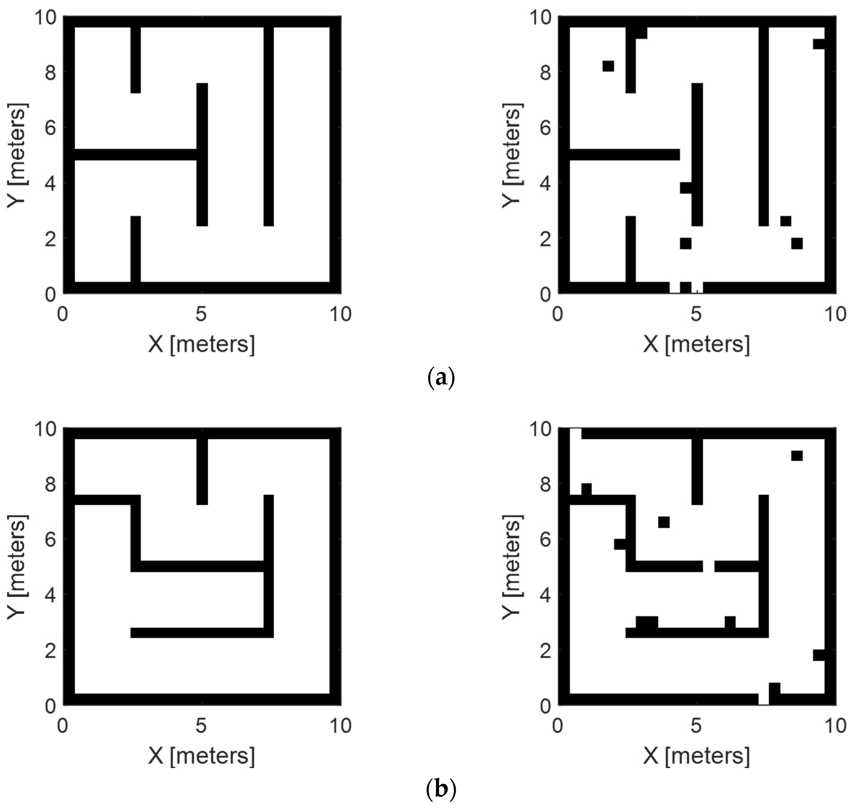
3.2. Validation of Environment Compression

The latent representation of the environment has a great impact on the final path planner performance since it incorporates all of the information of the map that the RL agent makes a decision on. If the compressed latent state of the environment can make the reconstructed map very close to the original map, then it is regarded as incorporating sufficient key information of the map representation.

We used the 200 generated maze maps as the training dataset. The size of the original input to the autoencoder was 25 × 25 (because the width of the map was 10 m and the resolution was 0.4 m, the size was 10 m/0.4 m = 25). For the encoder part, two consecutive CNN layers, whose kernel size was 3 × 3, padding was 1 on two sides, and stride step was 2, were used. Therefore, the latent representation of the environment was 7 × 7 after being processed by the CNN layers. Then, two transposed convolution layers with the same hyperparameters as the above CNN layer were used in the decoder network to resize the latent representation to the original size of the map. It needs to be highlighted here that because the original map was a binary occupancy map, i.e., each grid was 0 or 1, we also wanted the reconstructed map to have only two values. Therefore, a softmax layer was added to the decoder network, and then values higher than 0.5 were set to 1, while others are set to 0. The MSE error of the original and reconstructed maps at each pixel was defined as the loss to train the autoencoder.

Figure 5 demonstrates some examples of original and reconstructed maps. It needs to be highlighted here that the demonstration includes both training maps and testing maps that are not used in the autoencoder training. It can be seen that the reconstructed maps are very close to the original maps in both the training and testing scenarios, indicating the effectiveness and generalization ability of the trained autoencoder. The results show that the MSEs between the original and reconstructed maps are 0.0144 and 0.0192 on the training and testing datasets. Therefore, the latent state representation generated by the autoencoder can provide sufficient information for following path planning.

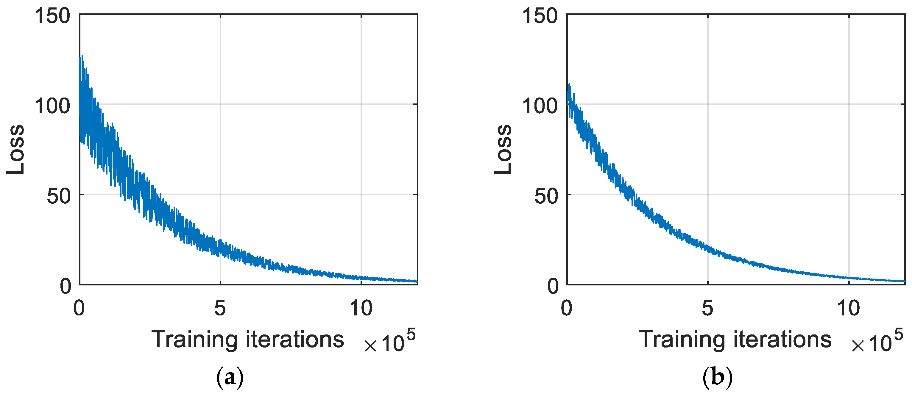
3.3. Validation of Transformer Encoder Feature Extraction

According to Section 3.2, the environment was represented as a 7 × 7 matrix. Therefore, its flattened form, namely a vector of size 49, was concatenated with the target point configuration, a vector of 3 (representing x, y, and orientation), to be fed into the IRL module directly. For the Transformer encoder, a time window with a length of 10 collecting corresponding UGV status information was set as the input. Here, four Transformer encoder layers were used, and each layer shared an embedding size of 24, a multi-head number of 3, and a feed-forward hidden layer size of 48. The Transformer encoder fully exploited the correlations among the UGV statuses during the last few time windows and passed the most essential information to the following IRL module. The reward r used by the IRL module is defined as

$$r\left(s_t,a_t\right)=-l(s_t,a_t)=-(\alpha e_x+\beta e_y)$$

(20)

where l represents the loss; $\alpha$ and $\beta$ represent the scaling coefficients; and e_x and e_y are the distances between predicted the target point and the recommended target point by the RRT* in the x and y directions, respectively. It can be seen from the above equation that the reward is the opposite of the loss, because we wanted to maximize the reward or minimize the loss. Here, we set $\alpha =\beta$ = 100.

In order to verify the effectiveness of the Transformer encoder’s feature-extraction ability, three representative network structures, namely CNN, GRU, and long short-term memory (LSTM) networks, were used as the benchmarks. Two evaluation metrics, including path length and smoothness, were used for comparison. Path length refers to the accumulated Euclidean distance of the waypoints on the path. Smoothness is defined according to Ref. [44], and measures the total amount of curvature along a path, and a lower smoothness value indicates a smoother path.

Table 1. Comparison between different network structures.

Network Structure	Path Length	Smoothness
CNN	18.96 m	7.43
GRU	18.21 m	6.13
LSTM	17.55 m	7.12
Transformer encoder	15.87 m	5.82

compares the results of the testing datasets. It can be seen from Table 1 that the proposed method using the Transformer encoder results in a 9.6~16.3% improvement in path length and a 5.1~21.7% improvement in smoothness.

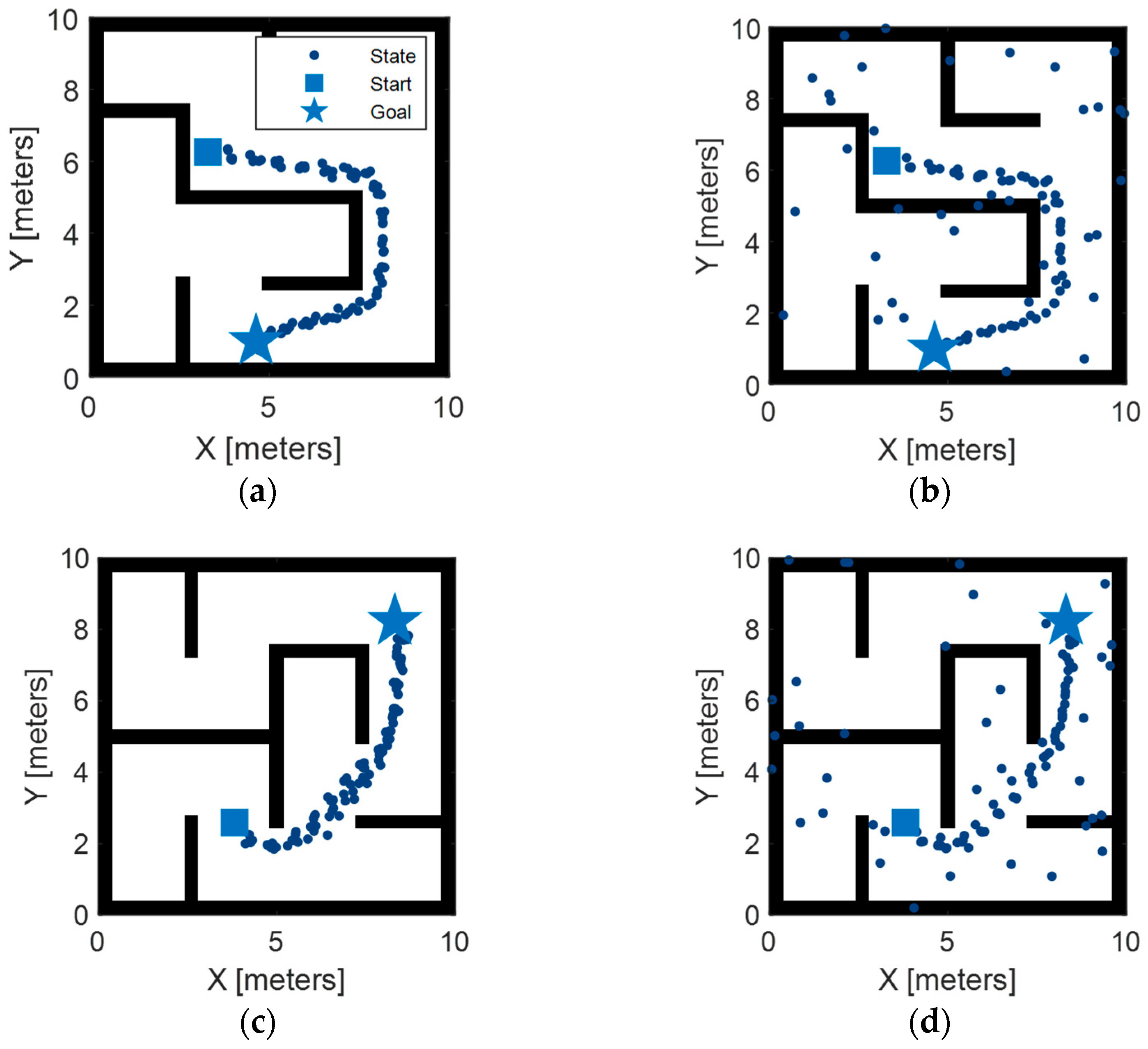
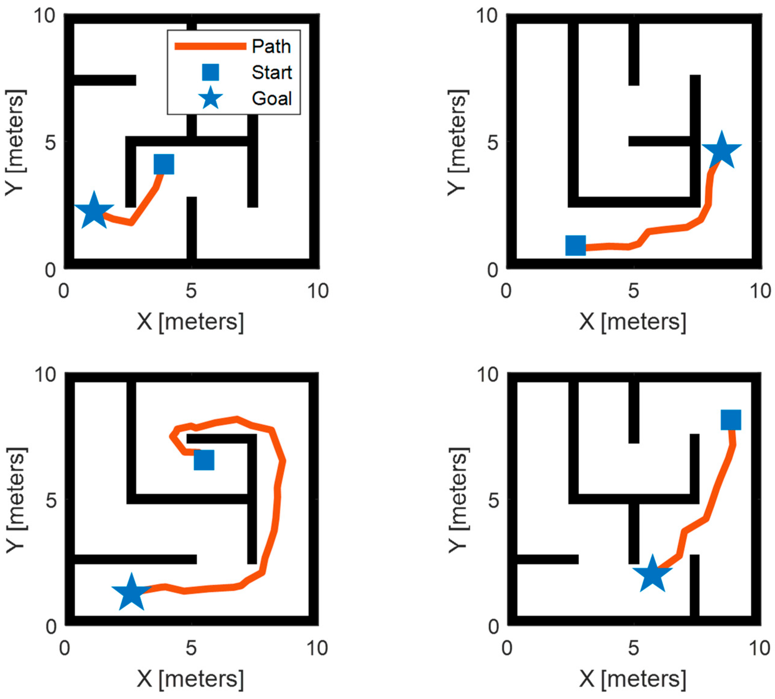
3.4. Validation of Effectiveness and Adaptability

Figure 6 demonstrates the loss of two networks, $M_{t^{\prime }}$ and M_t, during the training process. It can be seen from the figure that the losses of the two networks share a similar decreasing trend, which means the training is effective and the target point given by the proposed method is close to that of RRT*. It also needs to be highlighted here that the noise in the loss trend of M_t is smaller than that of $M_{t^{\prime }}$. This is because the $M_{t^{\prime }}$ network is the main network that interacts with the environment and uses the reward signal to improve the network performance, while the M_t network uses the parameters of $M_{t^{\prime }}$ as the training target. Therefore, the $M_{t^{\prime }}$ network already provides enough beneficial experience to the M_t network, thus saving it trial-and-error costs and demonstrating lower fluctuations in the loss curve.

In order to demonstrate the effectiveness of the proposed method, Figure 7 shows the target points generated by the proposed method in two representative scenarios, together with the partially traditional uniform sampling method for comparison, where r represents the ratio of the points generated by the proposed method to the total number of points. It can be seen from Figure 7 that if the target points are totally generated by the proposed method, namely r = 100%, all points are directly guiding the UGV towards the final goal point without redundant meaningless points. However, if partially uniform sampling is incorporated, some noise points deviating from the optimal path will appear, which would decrease the path-planning efficiency and optimality.

A typical example of the generated path for the traditional uniform sampling method and the proposed method is shown in Figure 8. It can be seen that the path of the proposed method is much shorter and smoother than that of the uniform sampling method. For a much fairer comparison, Figure 9 compares the two methods for 30 trails to exclude occasionality. The statistical metrics, including execution time, path length, and smoothness, are reported. It can be seen from Figure 9 that for the metrics of path length and smoothness, the proposed method wins a lot more than the uniform sampling method. As for the execution time, although the mean values of the two methods are similar, the proposed method has much lower deviation, indicating its robustness for different random settings.

The aforementioned simulation validates the efficacy of the proposed method under conditions resembling those of the training settings. However, real-world scenarios frequently diverge significantly from the datasets used for training, leading to a notable decline in the performance of trained agents when employing traditional fine-tuning-based transfer-learning techniques. In contrast, the proposed method embraces an incremental learning framework, enabling rapid adaptation to novel environments by leveraging the richly abstracted experiences gleaned from the training datasets. To substantiate this assertion, a notably complex environment, surpassing the complexity of the training datasets, is employed for verification, as depicted in Figure 10a. The corresponding training loss of both the traditional fine-tuning method and the proposed method is presented in Figure 10b. Notably, the proposed method demonstrates a fivefold increase in adaptivity compared to traditional transfer-learning approaches. For instance, achieving a loss of approximately 20 requires around 44,500 iterations with transfer learning, whereas the proposed method achieves this milestone in only 9000 iterations. Furthermore, the path generated by the proposed method, as illustrated in Figure 10a, exhibits smoothness and a rational path length, further affirming its efficacy.

4. Conclusions

This paper introduces a novel highly self-adaptive path-planning methodology grounded in Transformer encoder feature extraction and IRL. Out principal conclusions can be summarized across three key facets:

• The utilization of an autoencoder facilitates the generation of a compressed representation of the original environment, supplying ample information for subsequent path-planning endeavors while significantly reducing the computational overhead. The MSEs between the original and reconstructed maps amount to 0.0144 and 0.0192 on the training and testing datasets, respectively.
• Comparative evaluations reveal that the Transformer encoder exhibits superior feature-extraction capabilities in contrast to commonly utilized networks such as the CNN, GRU, and LSTM. Specifically, the proposed methodology employing the Transformer encoder yields a 9.6% to 16.3% enhancement in path length and a 5.1% to 21.7% improvement in smoothness.
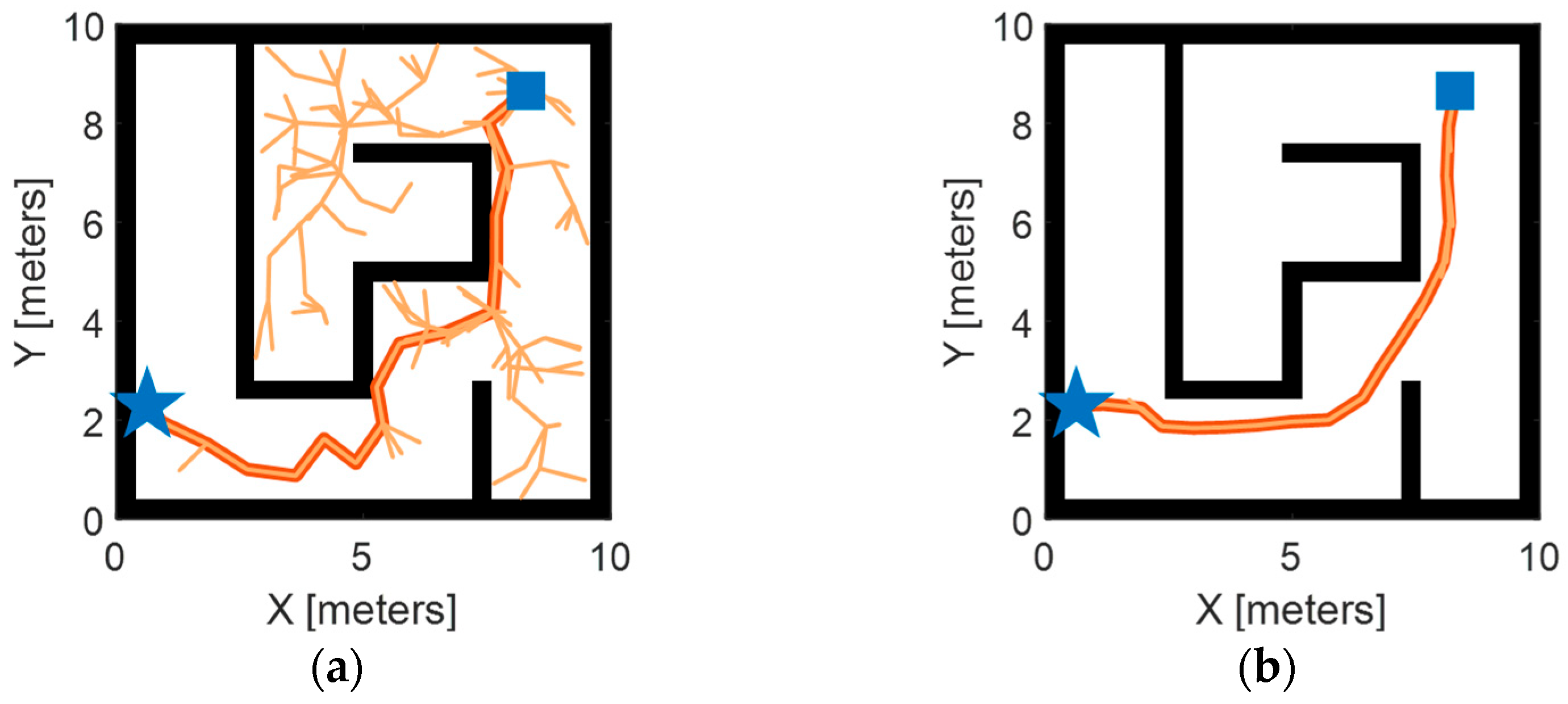
• The proposed methodology demonstrates superior optimality compared to uniform-sampling-based approaches and enhanced adaptability relative to traditional transfer-learning-based methodologies. Specifically, the proposed method exhibits a 14.8% reduction in path length and a 61.1% enhancement in smoothness compared to uniform-sampling-based approaches. Furthermore, leveraging incremental learning, the proposed method achieves adaptivity five times faster than traditional transfer-learning approaches.

In future endeavors, our primary objective will be to enhance the credibility and applicability of the proposed method through rigorous real-world testing conducted on a physical UGV. By transitioning from simulated environments to actual field tests, we intend to evaluate the method’s real-time performance and robustness under diverse practical scenarios like in [45]. Through meticulous data collection and analysis during these tests, we aim to not only validate the effectiveness of the proposed method but also identify any potential limitations or areas for improvement.

References

1. Dinelli, C.; Racette, J.; Escarcega, M.; Lotero, S.; Gordon, J.; Montoya, J.; Hassanalian, M. Configurations and applications of multi-agent hybrid drone/unmanned ground vehicle for underground environments: A review. Drones 2023, 7, 136. [Google Scholar] [CrossRef]
2. Sánchez, M.; Morales, J.; Martínez, J.L. Waypoint generation in satellite images based on a cnn for outdoor ugv navigation. Machines 2023, 11, 807. [Google Scholar] [CrossRef]
3. Fan, J.; Zhang, X.; Zheng, K.; Zou, Y.; Zhou, N. Hierarchical path planner combining probabilistic roadmap and deep deterministic policy gradient for unmanned ground vehicles with non-holonomic constraints. J. Frankl. Inst. 2024, 361, 106821. [Google Scholar] [CrossRef]
4. Dong, H.; Shen, J.; Yu, Z.; Lu, X.; Liu, F.; Kong, W. Low-Cost Plant-Protection Unmanned Ground Vehicle System for Variable Weeding Using Machine Vision. Sensors 2024, 24, 1287. [Google Scholar] [CrossRef] [PubMed]
5. Aggarwal, S.; Kumar, N. Path planning techniques for unmanned aerial vehicles: A review, solutions, and challenges. Comput. Commun. 2020, 149, 270–299. [Google Scholar] [CrossRef]
6. Liu, J.; Anavatti, S.; Garratt, M.; Abbass, H.A. Modified continuous ant colony optimisation for multiple unmanned ground vehicle path planning. Expert Syst. Appl. 2022, 196, 116605. [Google Scholar] [CrossRef]
7. Jones, M.; Djahel, S.; Welsh, K. Path-planning for unmanned aerial vehicles with environment complexity considerations: A survey. ACM Comput. Surv. 2023, 55, 1–39. [Google Scholar] [CrossRef]
8. Wang, H.; Li, G.; Hou, J.; Chen, L.; Hu, N. A path planning method for underground intelligent vehicles based on an improved RRT* algorithm. Electronics 2022, 11, 294. [Google Scholar] [CrossRef]
9. Chen, R.; Hu, J.; Xu, W. An RRT-Dijkstra-based path planning strategy for autonomous vehicles. Appl. Sci. 2022, 12, 11982. [Google Scholar] [CrossRef]
10. Wang, J.; Chi, W.; Li, C.; Wang, C.; Meng MQ, H. Neural RRT*: Learning-based optimal path planning. IEEE Trans. Autom. Sci. Eng. 2020, 17, 1748–1758. [Google Scholar] [CrossRef]
11. Chen, P.; Pei, J.; Lu, W.; Li, M. A deep reinforcement learning based method for real-time path planning and dynamic obstacle avoidance. Neurocomputing 2022, 497, 64–75. [Google Scholar] [CrossRef]
12. Yu, X.; Wang, P.; Zhang, Z. Learning-based end-to-end path planning for lunar rovers with safety constraints. Sensors 2021, 21, 796. [Google Scholar] [CrossRef] [PubMed]
13. Park, B.; Choi, J.; Chung, W.K. An efficient mobile robot path planning using hierarchical roadmap representation in indoor environment. In Proceedings of the 2012 IEEE International Conference on Robotics and Automation, St Paul, MN, USA, 14–19 May 2012; IEEE: New York, NY, USA, 2012; pp. 180–186. [Google Scholar]
14. Deng, Y.; Chen, Y.; Zhang, Y.; Mahadevan, S. Fuzzy Dijkstra algorithm for shortest path problem under uncertain environment. Appl. Soft Comput. 2012, 12, 1231–1237. [Google Scholar] [CrossRef]
15. Arogundade, O.T.; Sobowale, B.; Akinwale, A.T. Prim algorithm approach to improving local access network in rural areas. Int. J. Comput. Theory Eng. 2011, 3, 413. [Google Scholar]
16. Lee, W.; Choi, G.H.; Kim, T.W. Visibility graph-based path-planning algorithm with quadtree representation. Appl. Ocean. Res. 2021, 117, 102887. [Google Scholar] [CrossRef]
17. Kavraki, L.E.; Kolountzakis, M.N.; Latombe, J.C. Analysis of probabilistic roadmaps for path planning. IEEE Trans. Robot. Autom. 1998, 14, 166–171. [Google Scholar] [CrossRef]
18. Sun, Y.; Zhao, X.; Yu, Y. Research on a random route-planning method based on the fusion of the A* algorithm and dynamic window method. Electronics 2022, 11, 2683. [Google Scholar] [CrossRef]
19. Wu, J.; Ma, X.; Peng, T.; Wang, H. An improved timed elastic band (TEB) algorithm of autonomous ground vehicle (AGV) in complex environment. Sensors 2021, 21, 8312. [Google Scholar] [CrossRef]
20. Reinhart, R.; Dang, T.; Hand, E.; Papachristos, C.; Alexis, K. Learning-based path planning for autonomous exploration of subterranean environments. In Proceedings of the 2020 IEEE International Conference on Robotics and Automation (ICRA), Paris, France, 31 May–31 August 2020; IEEE: New York, NY, USA, 2020; pp. 1215–1221. [Google Scholar]
21. Kulathunga, G. A reinforcement learning based path planning approach in 3D environment. Procedia Comput. Sci. 2022, 212, 152–160. [Google Scholar] [CrossRef]
22. Chen, G.; Pan, L.; Xu, P.; Wang, Z.; Wu, P.; Ji, J.; Chen, X. Robot navigation with map-based deep reinforcement learning. In Proceedings of the 2020 IEEE International Conference on Networking, Sensing and Control (ICNSC), Nanjing, China, 30 October–2 November 2020; IEEE: New York, NY, USA, 2020; pp. 1–6. [Google Scholar]
23. Wang, X.; Shang, E.; Dai, B.; Nie, Y.; Miao, Q. Deep Reinforcement Learning-based Off-road Path Planning via Low-dimensional Simulation. IEEE Trans. Intell. Veh. 2023. [Google Scholar] [CrossRef]
24. Fan, J.; Zhang, X.; Zou, Y. Hierarchical path planner for unknown space exploration using reinforcement learning-based intelligent frontier selection. Expert Syst. Appl. 2023, 230, 120630. [Google Scholar] [CrossRef]
25. Zhang, L.; Cai, Z.; Yan, Y.; Yang, C.; Hu, Y. Multi-agent policy learning-based path planning for autonomous mobile robots. Eng. Appl. Artif. Intell. 2024, 129, 107631. [Google Scholar] [CrossRef]
26. Cui, Y.; Hu, W.; Rahmani, A. Multi-robot path planning using learning-based artificial bee colony algorithm. Eng. Appl. Artif. Intell. 2024, 129, 107579. [Google Scholar] [CrossRef]
27. Sartori, D.; Zou, D.; Pei, L.; Yu, W. CNN-based path planning on a map. In Proceedings of the 2021 IEEE International Conference on Robotics and Biomimetics (ROBIO), Sanya, China, 6–9 December 2021; IEEE: New York, NY, USA, 2021; pp. 1331–1338. [Google Scholar]
28. Jin, X.; Lan, W.; Chang, X. Neural Path Planning with Multi-Scale Feature Fusion Networks. IEEE Access 2022, 10, 118176–118186. [Google Scholar] [CrossRef]
29. Qureshi, A.H.; Miao, Y.; Simeonov, A.; Yip, M.C. Motion planning networks: Bridging the gap between learning-based and classical motion planners. IEEE Trans. Robot. 2020, 37, 48–66. [Google Scholar] [CrossRef]
30. Bae, H.; Kim, G.; Kim, J.; Qian, D.; Lee, S. Multi-robot path planning method using reinforcement learning. Appl. Sci. 2019, 9, 3057. [Google Scholar] [CrossRef]
31. Wang, M.; Zeng, B.; Wang, Q. Research on motion planning based on flocking control and reinforcement learning for multi-robot systems. Machines 2021, 9, 77. [Google Scholar] [CrossRef]
32. Huang, R.; Qin, C.; Li, J.L.; Lan, X. Path planning of mobile robot in unknown dynamic continuous environment using reward-modified deep Q-network. Optim. Control. Appl. Methods 2023, 44, 1570–1587. [Google Scholar] [CrossRef]
33. Akkem, Y.; Biswas, S.K.; Varanasi, A. A comprehensive review of synthetic data generation in smart farming by using variational autoencoder and generative adversarial network. Eng. Appl. Artif. Intell. 2024, 131, 107881. [Google Scholar] [CrossRef]
34. Li, P.; Pei, Y.; Li, J. A comprehensive survey on design and application of autoencoder in deep learning. Appl. Soft Comput. 2023, 138, 110176. [Google Scholar] [CrossRef]
35. Fan, J.; Zhang, X.; Zou, Y.; He, J. Multi-timescale Feature Extraction from Multi-sensor Data using Deep Neural Network for Battery State-of-charge and State-of-health Co-estimation. IEEE Trans. Transp. Electrif. 2023. [Google Scholar] [CrossRef]
36. Gao, H.; Yuan, H.; Wang, Z.; Ji, S. Pixel transposed convolutional networks. IEEE Trans. Pattern Anal. Mach. Intell. 2019, 42, 1218–1227. [Google Scholar] [CrossRef]
37. Vaswani, A.; Shazeer, N.; Parmar, N.; Uszkoreit, J.; Jones, L.; Gomez, A.N.; Polosukhin, I. Attention is all you need. Adv. Neural Inf. Process. Syst. 2017, 30. [Google Scholar] [CrossRef]
38. Li, J.; Wang, X.; Tu, Z.; Lyu, M.R. On the diversity of multi-head attention. Neurocomputing 2021, 454, 14–24. [Google Scholar] [CrossRef]
39. Cui, B.; Hu, G.; Yu, S. Deepcollaboration: Collaborative generative and discriminative models for class incremental learning. In Proceedings of the AAAI Conference on Artificial Intelligence, Vancouver, BC, Canada, 2–9 February 2021; Volume 35, pp. 1175–1183. [Google Scholar]
40. Haarnoja, T.; Zhou, A.; Hartikainen, K.; Tucker, G.; Ha, S.; Tan, J.; Levine, S. Soft actor-critic algorithms and applications. arXiv 2018, arXiv:1812.05905. [Google Scholar]
41. Fan, J.; Ou, Y.; Wang, P.; Xu, L.; Li, Z.; Zhu, H.; Zhou, Z. Markov decision process of optimal energy management for plug-in hybrid electric vehicle and its solution via policy iteration. J. Phys. Conf. Ser. 2020, 1550, 042011. [Google Scholar] [CrossRef]
42. Luong, M.; Pham, C. Incremental learning for autonomous navigation of mobile robots based on deep reinforcement learning. J. Intell. Robot. Syst. 2021, 101, 1. [Google Scholar] [CrossRef]
43. Yang, Z.; Zeng, A.; Li, Z.; Zhang, T.; Yuan, C.; Li, Y. From knowledge distillation to self-knowledge distillation: A unified approach with normalized loss and customized soft labels. In Proceedings of the IEEE/CVF International Conference on Computer Vision, Paris, France, 2–6 October 2023; pp. 17185–17194. [Google Scholar]
44. Smoothness of Path—MATLAB Smoothness. Available online: https://ww2.mathworks.cn/help/nav/ref/pathmetrics.smoothness.html (accessed on 1 March 2024).
45. Simon, J. Fuzzy control of self-balancing, two-wheel-driven, SLAM-based, unmanned system for agriculture 4.0 applications. Machines 2023, 11, 467. [Google Scholar] [CrossRef]
Figure 1. General framework of the proposed path-planning method.
Machines 12 00289 g001
Figure 2. Overall structure of the autoencoder.
Machines 12 00289 g002
Figure 3. Attention mechanism in Transformer encoder layer. (a) Scaled dot-product attention; (b) multi-head attention. Reprinted with permission from Ref. [37]. 2017, Vaswani, A. et al.
Machines 12 00289 g003
Figure 4. Generated maze maps and demonstration path.
Machines 12 00289 g004
Figure 5. Comparison between original maps and reconstructed maps. (a) Example on training map dataset; (b) example on testing map dataset.
Machines 12 00289 g005
Figure 6. Training loss trend for the two networks. (a) Training loss for M t network; (b) training loss for Mt network.
Machines 12 00289 g006
Figure 7. Comparison of the proposed method and random sampling. (a) Configuration 1 with r = 100%; (b) configuration 1 with r = 60%; (c) configuration 2 with r = 100%; (d) configuration 2 with r = 60%.
Machines 12 00289 g007
Figure 8. Comparison of generated paths using proposed method and uniform sampling. (a) Uniform sampling; (b) proposed method.
Machines 12 00289 g008
Figure 9. Metrics comparison of proposed method and uniform sampling over 30 trails. (a) Examples of 30 trails; (b) execution time; (c) path length; (d) smoothness.
Machines 12 00289 g009
Figure 10. Validation of the proposed method on a complicated map. (a) Complicated map and generated path; (b) loss curve.
Machines 12 00289 g010