Abstract
Unmanned ground vehicles (UGVs) have gained increased attention in different fields of application; therefore, their optimization requires special attention. Lowering the mass of a UGV is especially important to increase its autonomy, agility, and payload capacity and to reduce dynamic forces. This contribution deals with optimizing a UGV unit prototype that, when connected with similar units, forms a moving electric fence for animal grazing. Together, these units form a robotic system that is intended to solve the critical problem of lack of human capacity in herding and grazing. This approach employs topology optimization (TO) and finite element analysis (FEA) to lower the mass of a UGV unit and validate the design of its structural components. To our knowledge, no optimization of this type of UGV has been reported in the literature. Here, we present the results of a case study in which a set of four load cases served as a basis for the optimization of the UGV frame. Response surface analysis (RSA) was used to identify the worst load cases, while substructuring was used to allow for more detailed meshing of the frame portion that was subjected to TO. Thereby, we demonstrate that the prototype of the UGV unit can be built using standard parts and that TO and FEA can be efficiently used to optimize the load-carrying structure of such a specific vehicle.
1. Introduction
In recent years, the use of unmanned ground vehicles (UGVs) has significantly affected various industrial sectors. The agricultural sector has also experienced a notable transformation owing to the employment of UGVs for activities such as crop monitoring, spraying, and harvesting, contributing to improved efficiency and decreased labor costs [1,2].
In agriculture, UGVs have also been utilized to serve a potentially more challenging duty than plant growth: animal husbandry. Animal herding and grazing are particularly challenging tasks within the domain of animal husbandry because of the inherent need for livestock to constantly move from stables to grazing areas and back, as well as to move within grazing areas. Existing herding solutions often rely on mimicking guarding animals, such as shepherd dogs, thereby also using unmanned aerial vehicles (UAVs). Whereas King et al. [3] used a synchronized pair of UAVs, Li et al. introduced a robotic animal herding system utilizing a network of autonomous barking drones [4].
The increasing interest in UGVs across various sectors necessitates special attention to their optimization, which generally involves enhancing their structural design and capabilities for specific industries and tasks. Here, we focus on the demands that define the load-carrying structure of a UGV unit. In the context of grazing and herding, UGVs must meet specific structural demands, including:
- Robustness: UGVs used for grazing and herding must be built to withstand rough terrain, varying weather conditions, and potential livestock impacts. A robust chassis is a necessity in this context.
- Agility: UGVs should be designed to easily maneuver through fields and pastures, allowing them to follow livestock herds or avoid obstacles.
- Payload Capacity: This demand is essential for UGVs that carry equipment for distributing feed, monitoring livestock health, or collecting data on grazing patterns.
- Energy Efficiency: Given the potential for UGVs to operate over large areas for extended periods, energy efficiency is crucial. The battery capacity, charging infrastructure, and power management systems should be designed to maximize the operational time of the vehicle.
To meet the demands mentioned above, designers often use structural analysis [5] and optimization [6] in the design process. The obvious advantage of structural optimization is that it enables searching for the “best” design, whereas structural analysis only enables validation of an existing design. Parametric optimization (PO) and topology optimization (TO) [7] are two prevalent forms of structural optimization, each with distinct strengths and weaknesses [8]. Currently, both structural analysis and optimization rely heavily on finite element analysis (FEA) [9] as a virtual experimentation technique. TO is frequently used as a tool for lightweighting, a strategic approach aimed at achieving a desired function with minimal mass, within set constraints [10].
Gadekar et al. used static structural analysis to validate the chassis design of a modular UGV for surveillance and logistics operations [11]. A similar approach was used by Mohebbi et al. to check the stress state of critical parts of the tracked surveillance UGV for missions in hazardous environments [12], and by Vardin et al. to validate chassis and wheel hub assemblies of a UGV for off-road applications [13].
Wildman and Gaynor [14] bring an overview of various TO techniques used in robotics, and an example of TO applied to the flipper component on the iRobot Packbot Army platform. Demir et al. used TO to reduce the mass of a mobile transportation robot [15]. Banić et al. used TO and static structural analysis to lower the weight of a prototype of a battery-powered robot UGV, named Agriculture Autonomous Robot (AgAR) [10]. The robot was specifically designed for both indoor and outdoor operations, with a special focus on precision agriculture. The loads used in the optimization process were obtained from a digital twin. Literature contributions related to the structural optimization of UGVs are rather rare; however, papers may be found related to robotics in general or vehicle design, where lightweighting is also of great importance (e.g., [16,17,18,19]).
We present a novel mobile robotic fence named RoboShepherd, designed to guide livestock to grazing areas and define grazing limits. It consists of UGV units that are mutually connected by wires to form a moving fence for animal grazing. In this way, the number of people needed to care for livestock is further reduced, enabling the entire livestock management process to take place on the farm where the stables are situated. The innovative solution, currently at technology readiness level (TRL) 6 and with pending patent approval, was collaboratively developed by Coming Computer Engineering and the Faculty of Mechanical Engineering at the University of Niš. The technology readiness level is a measurement system used to assess the maturity level of a particular technology [20]. On the technology readiness scale, TRL 6 represents a technology demonstrated in a relevant environment, which aligns with the current stage of development of the RoboShepherd system. The RoboShepherd system underwent a three-month testing period at three farms in Serbia, managing flocks of up to 300 animals that grazed along their usual pasturing routes using the system. Since the system was tested with animals moving along the actual pastures on a predefined grazing route, it can be considered that the system was demonstrated in a relevant environment.
This study focuses on the structural optimization of a prototype robotic unit (UGV) within a RoboShepherd system. Our approach involves employing TO and FEA to decrease the mass of the UGV unit and to validate the design of its structural components. The response surface analysis (RSA) is used to identify the worst load cases. Submodeling is employed to analyze the UGV frame, allowing for a more detailed finite element (FE) mesh to be used in the TO process. In this case study, a set of four load cases identified as the worst ones served as the foundation for TO, based on which a modified CAD model of the UGV frame was created. Consequently, the mass of the UGV frame was reduced by 30.7%. To the best of our knowledge, there is no documented optimization of this type of UGV or optimization of any structure performed using a methodology identical to the one described here. By presenting the study, we demonstrate the feasibility of constructing a prototype UGV unit using standard parts and highlight the effectiveness of the presented methodology in optimizing the load-bearing structure of such a specialized vehicle.
2. Materials and Methods
2.1. RoboShepherd–Automated Animal Husbandry and Grazing System
RoboShepherd is a robotic system composed of multiple interconnected robots, as illustrated in Figure 1. It operates as a mobile polygonal electric barrier encircling livestock in the field, directing them along predetermined routes. The system consists of at least four robotic units that create a wire electric fence that, when necessary, emits a high-voltage pulse to deter animals. When animals touch the fence, harmless shock redirects them. The electric fence also serves as a protection against predators. The system is designed for easy replication and can be adapted to different animal types and regions by adding more robotic units.
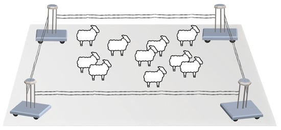
Figure 1.
RoboShepherd: A moving electrical fence for herding and grazing.
Each RoboShepherd robotic unit (UGV) is a versatile mobile platform powered by a battery and equipped with wheels to navigate both land and shallow water terrains. The UGV is primarily devised for outdoor operation on landscaped pastures, featuring slopes up to 30%. This, however, implies a substantial ability to traverse rocky fields, soft ground, low vegetation areas, and muddy terrain. What sets this UGV apart from other robotic grazing solutions is its unique method of connecting UGV units through wires to create a mobile fence. This design approach influences specific features of the UGV units, such as vertical posts, a wire tensioning system, minimal vehicle ground clearance, and a short distance from the lowest wire to the ground. Consequently, each robotic unit comprises three primary subassemblies: a mobile platform, vertical post, and wire tensioning system (Figure 2). The wire tensioning system consists of two primary subassemblies: the wire connection and the wire tensioning device. Further details regarding the design, operational principles, control system, and system testing of RoboShepherd will be presented in a forthcoming paper currently under preparation.
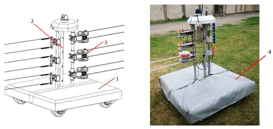
Figure 2.
Main subassemblies of the RoboShepherd robotic unit: (1) mobile platform, (2) vertical post and (3) wire tensioning system. The waterproof and thermal insulating jacket (4) is shown in the right image.
2.2. Optimization Method
Structural optimization typically involves enhancing the strength or stiffness of engineering structures while minimizing their weight or cost. Four groups of structural optimization problems can be distinguished: optimization of dimensions, shape optimization, topology optimization (TO), and material optimization [21]. Shape optimization can involve adjusting the node locations within the FE mesh or modifying the parameters of the CAD model that forms the basis of the FE model (referred to as parametric optimization, PO).
PO relies on methods such as the design of experiments (DOE), response surfaces, and mathematical optimization, to find a set of optimal values of chosen design variables that yield the “best” solution by minimizing or maximizing one or more goal functions [6]. In PO, design variables define the outer and inner contour lines (shape) of the structure but new structural elements such as cavities or ribs cannot be added (it is not possible to change topology). TO represents the most general form of structural optimization because it affects the dimensions and shape of the structure. In TO, a part is most often treated as a set of building blocks that can disappear and reappear. Emphasis is placed on removing the blocks that are least loaded, to reduce the mass of the structure. If TO is based on the FE model, these blocks correspond to finite elements.
There are various TO methods, density-based being the oldest and most used. It represents the material distribution within a design space using a density field. This means assigning a density value to each point in the design domain, where high density indicates the presence of material and low density indicates void space [6,22]. Another popular method is level-set-based optimization, which uses level-set functions to represent the geometry of the design. Level-set functions are signed distance functions that can capture complex shapes and boundaries [22]. In an author’s previous works, it was used for solving inversion problems [23,24]. While the former is easier to implement and allows more arbitrary changes in topologies, the latter provides a well-defined material boundary and may converge faster. The mixable-density approach, as implemented in Ansys 2023 R1, is an expanded reiteration of the density-based method with the goal of providing equivalent functionalities alongside enhancements to these features. It is declared to deliver smoother results and integrate the advantages of other methods [25].
TO is known to produce organic shapes that, as geometric objects, are not suitable for editing (Figure 3). Thus, a TO workflow typically applied in many commercial software packages implies building the parametric CAD model, creating an FE model based on the CAD model, performing structural analysis, performing TO to obtain an optimized polygonal model, building the new parametric CAD model based on the topologically optimized one (semi-automatically), and validating the new CAD model using another structural analysis [26].
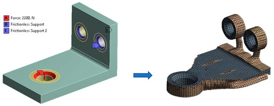
Figure 3.
Topology optimization of a wall bracket, where stiffness maximization was set as the goal, and 50% mass reduction was set as a design constraint.
There also exists a possibility to further improve the topology-optimized model using PO. For example, Ismail et al. employed PO after TO to further reduce the stresses at sharp corners created within a prototype of a bicycle crank arm [27]. Tyflopoulos et al. performed a comprehensive comparative study of the application of PO, TO, and various procedures that combine both approaches in lightweighting a simple structure [8]. Although they did not specify a particular method as superior, they did highlight certain preferred approaches when the goals are reducing mass or shortening optimization time.
RoboShepherd UGV Unit Optimization Constraints and Workflow
An essential aspect of the RoboShepherd project was the rapid development of the initial prototype for real-world testing. To streamline the manufacturing process and ensure cost-effectiveness, the choice was made to utilize standard profiles and parts predominantly. Standard steel profiles were welded together to construct the load-bearing frame. Steel and aluminum plates were also used in other subassemblies. Commercial parts were incorporated into the wheel assemblies and wherever possible, except for the wire tensioning system coils, which were 3D printed. Laser cutting was used to produce polygonal cuts on the steel profiles.
The primary operational requirements for the RoboShepherd UGV unit included agility, energy efficiency, and durability. To meet these demands, lightweighting was performed. This was also beneficial for reducing dynamic forces affecting the UGV. The “payload capacity” requirement was irrelevant in this case, as the unit was not intended to transport any additional cargo. Rather, the most severe loading conditions were used to determine the UGV load capacity, taking into account animal interaction with wires, the weight of the vehicle, and measured dynamic forces, as described in Section 2.4. To identify these conditions, RSA was employed.
Before defining the optimization workflow for the RoboShepherd design system, specific constraints were established, including an operational range of 10 km. These constraints were influenced not only by the weight of the UGV but also by factors such as terrain, UGV movement patterns, battery capacity, temperature, and other similar conditions. These constraints could not be directly applied in the lightweighting process. Instead, the optimization goal was set to reduce the UGV mass by a feasible amount while adhering to the concept of utilizing standard parts and employing simple and cost-effective manufacturing methods. The initial mass of the structure to be optimized, excluding shields and electronic components, was 253.97 kg. Depending on the specific electronic components utilized, the additional mass of the UGV ranged from 40 kg to 50 kg, resulting in an overall mass approaching 300 kg.
Having in mind the goals and constraints mentioned above, the procedure for optimization of the UGV unit prototype was outlined as follows:
- Creation of CAD and finite element (FE) models of the UGV unit based on the initial concept.
- Definition of design variables within CAD and FE models and establishment of bidirectional associativity between the two.
- Performance of structural static analyses, RSA, and mathematical optimization to determine UGV unit configurations that can be subjected to the worst loading scenarios.
- Decision on structural optimization approach, based on the stress-strain state of UGV unit components within worst loading scenarios. The choice of whether PO, TO, or both would be employed, depending on whether a part of the structure should be strengthened or whether weight reduction within some of UGV subassemblies is possible.
- Modification of UGV unit design, according to the results of PO, TO, or both.
- Final static structural analysis and RSA to validate the new design.
- An RSA based on nonlinear eigenvalue buckling analyses, to address any concerns about the potential buckling of slender components in the optimized UGV design.
During the optimization process, it was also decided that substructuring (a.k.a. sub-modeling) [25] would be used to simplify and reduce the FE model of the UGV unit by keeping only its portions that were subjected to TO. This enabled the use of a more detailed mesh for the TO process. Also, this allowed for the correct loading conditions to be kept on the master model, where they acted on assembly components other than those being subjected to TO, while the loading was transferred to the submodel via cut boundaries. The importance of load being imposed on the assembly and not on single parts being topologically optimized is discussed by Sha et al. [16]. The additional substructuring benefit was related to avoiding geometric nonlinearity in the FE model of the optimization region, as explained in the Discussion.
2.3. CAD Model of UGV Assembly
The optimization process started with the creation of a simplified CAD model (Figure 4) that would serve as the basis for FE model building. All the components with a negligible contribution to structural stiffness, such as electronic modules, cables, and sensors, were removed. The dome, serving to shield electronic components from environmental factors, was omitted. The geometrical model of the gearbox and motor for wire tensioning was also simplified. The fasteners were removed to reduce computational demands and obtain FEA results in a reasonable time without significant loss of accuracy. As the shields did not contribute significantly to structural stiffness, they were also eliminated from the model. Simple rectangular objects were created to represent the ground. To accommodate the highest anticipated load on the UGV, a maximum of three tensioning devices and three sensors were placed on every pillar of the vertical post.
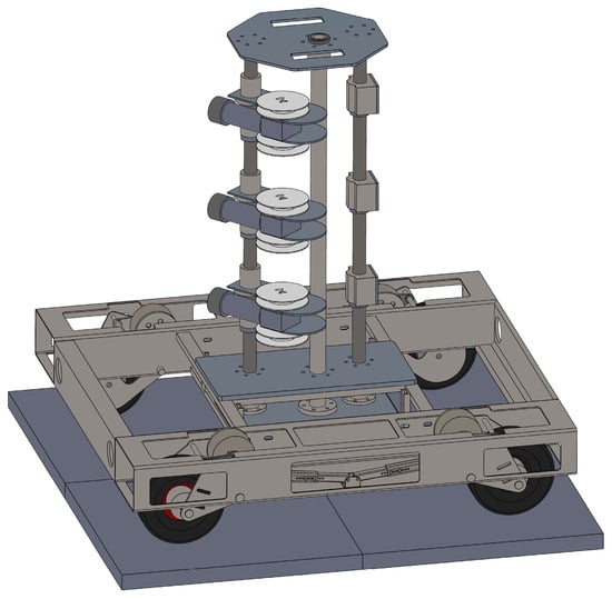
Figure 4.
Simplified CAD model of the UGV unit. The displayed configuration corresponds to the values of design variables DV1 and DV2 of 45° and 180°, respectively.
The CAD model was parametrized to facilitate the creation of different assembly configurations, which would serve as the basis for RSA or PO studies. The following design variables were defined, and the corresponding global variables were created in SolidWorks 2023:
- The angle of wires attached to winding coils, ranging from 45° to 315° (“DV1: Motoreductor angle” in Figure 5).
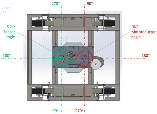 Figure 5. Design variables control the angle of wires attached to winding coils and the angle of wires attached to sensors. The picture shows the model in which the values of both variables are set to 180°.
 - The angle of wires attached to sensors, ranging from 45° to 315° (“DV2: Sensor angle” in Figure 5).
- The height of the lowest wires, i.e., of the mid-plane of wires 1 and 2 (“DV3” in Figure 6).
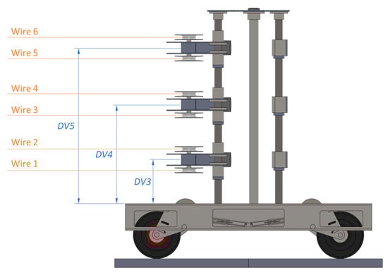 Figure 6. Design variables (DV3–DV5) controlling the height of wires (via the height of winding coils and sensors). Each design variable controls the height of two wires connected to one motoreductor.
 - The height of central wires, i.e., of the mid-plane of wires 3 and 4 (“DV4” in Figure 6).
- The height of the highest wires, i.e., of the mid-plane of wires 5 and 6 (“DV5” in Figure 6).
- The diameter of wires in the winding coil, i.e., the diameter of the circle containing the point at which a wire is leaving the coil (“DV6” in Figure 7).
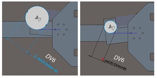 Figure 7. Design variable controlling the diameter of wires in the winding coil (DV6). This is achieved by modifying the diameter of the coil to simplify later definition of loads in FEA. The angle of the winding coil subassembly is automatically adjusted after each diameter change to keep the angle of wires equal to the value of DV1 (motoreductor angle), which in this image equals 180°.
2.4. Finite Element (FE) Model of UGV Assembly
The simplified geometric model of the UGV unit (Figure 4) was transformed into the FE model using advanced meshing tools. The discretized model (Figure 8) consisted of 954,684 nodes, forming 291,328 finite elements with quadratic shape functions. Joint and spring elements were added to simulate four shock absorbers, one of each in every wheel subassembly. The properties of materials used in the analysis are given in Table 1.
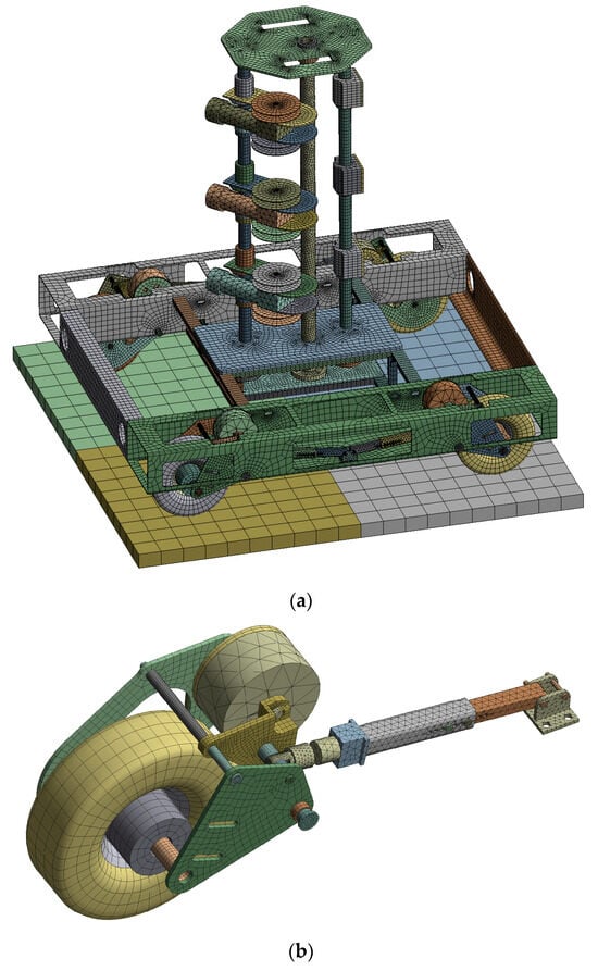
Figure 8.
(a) Discretized structure of the whole UGV assembly; (b) discretized structure of wheel subassembly. Different parts are shown in various colors, for clarity.

Table 1.
Properties of materials used in FEA of UVG assembly.
Steel S355 was used for frame components and pillars, aluminum 5754 H111 for all plates within vertical post subassembly, PLA for coils, and C45 for axles, pins, and sleeves. The material assigned to tires was originally solid wheel rubber. Its properties were changed to resemble plastic material, to achieve a much quicker convergence in FEA while keeping a similar stress state of the assembly. The material model of the ground was based on asphalt properties, without considering density, to exclude it from mass calculations. Motoreductor parts were assigned fictive material properties, where density was adjusted to yield the mass of the original motoreductor assembly when multiplied by part volume.
Contacts between frame parts, which are joined by bolted connections or by welding, were defined as “bonded” via multi-point constraint (MPC) formulation. The connections between moving parts were modeled using frictional contact, with a coefficient of friction varying from 0.1 to 0.2. The contact stiffness was updated in each FEA iteration.
Measurements showed that the UGV assembly is subjected to increased dynamic loads originating from the movement of the robotic unit on the rough terrain. The accelerations of the robotic unit frame were recorded by an inertial measurement unit (IMU) sensor that was positioned on the pillar base plate. A maximum load of 1.2 G was recorded at a maximum robotic unit speed (see Figure 9). An additional 0.1 G was considered to compensate for the weight of the excluded components. To simulate a total acceleration of 1.3 G, the additional 0.3 G acceleration load was combined with the standard gravity load.
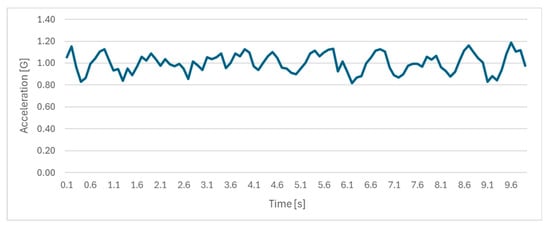
Figure 9.
Acceleration of UGV frame measured by IMU sensor.
The wire tensioning force acting on coils was limited to 80 N, as the noted force value was sufficient to ensure good wire tensioning at the maximal distance between the robotic units of 50 m [28]. Any additional increase in force beyond this threshold was deemed unnecessary as it would only result in added loads without any benefits to wire tensioning. The movement of components representing the ground was constrained in all directions. While the two wheels on one side of the UGV were defined as freely spinning, the rotation of the other two was prevented by constraining rotational degrees of freedom on brake surfaces. This setup aimed to simulate a real-world scenario involving the activation of wheel brakes.
In summary, the following loads and boundary conditions were defined on the FE model of the UGV unit (Figure 10):
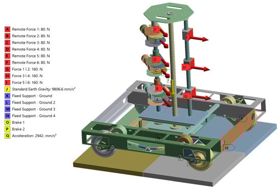
Figure 10.
Boundary conditions for static structural analysis of UGV assembly at increased dynamic loads. Different parts are shown in various colors, for clarity.
- tensioning force of 80 N acting on the winding coil (A–F)
- tensioning force of 160 N originating from tensioning of wires from another robotic unit (G–I)
- standard earth gravity (J)
- fixation of four parts representing ground (K–N)
- disk brakes applied on two wheels (O, P)
- acceleration of 0.3 G (Q)
The configuration shown in Figure 10 is the one corresponding to the motoreductor angle of 180° and sensor angle of 315°, evenly distributed wire heights, and maximum winding diameter. This specific configuration was determined to provide the highest value of maximum frame stress, as detailed in Section 3.
Models Used in Substructuring
Topology optimization was conducted on a submodel consisting of a section of the UGV frame, specifically of four large steel profiles (see Figure 11a). The smaller C-shaped profiles directly supporting the column subassembly were excluded from the frame subassembly, as their optimization was not considered practical. Surface imprints were made on the large rectangular profiles to indicate connections with the removed profiles, as depicted in Figure 11b. These imprints were used to transfer the displacements from the master model to the submodel. Displacements from the master model were also transferred to the submodel via cut boundaries created by removing small rectangular sections of the large profiles around the wheel axle holes and around the brackets belonging to the UGV height adjustment system (see Figure 11b). The removed volumes were therefore not considered in the TO. This was deemed acceptable because of their proximity to the contact regions between large rectangular profiles and other UGV components, which had to be preserved.

Figure 11.
(a) CAD model of UGV frame used in submodeling, (b) imprints and cut boundaries used for transfer of displacements from master model to submodel: (1) connections with the removed profiles, (2) removed rectangular sections around axle holes, (3) removed rectangular sections around height adjustment brackets.
A fine uniform mesh of quadratic tetrahedrons, with a typical element side of 3.5 mm, was created on the submodel according to recommendations of the software manufacturer [25], as shown in Figure 12.
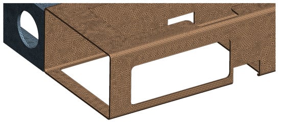
Figure 12.
A very fine FE mesh, created on the submodel.
3. Results
3.1. FEA of UGV Assembly and Response Surface Analysis (RSA)
According to the optimization workflow described in Section RoboShepherd UGV Unit Optimization Constraints and Workflow, the FE model of UGV assembly was used to assess UGV stress levels and identify components suitable for optimization. Out of the six design variables depicted in Figure 5, Figure 6 and Figure 7, the values of four were kept constant during the FE analysis. Within the UGV configuration containing three rows of double wires (Figure 10), the three variables defining wire heights (DV3, DV4, and DV5 in Figure 6) were set to specific values corresponding to the even distribution of wire pairs along column height (246 mm, 554 mm, and 872 mm, respectively). Such a configuration resulted in the maximum predicted sum load acting on the UGV column. The variable defining the diameter of wires in the winding coil (DV6 in Figure 7) was assigned the maximum value of 160 mm, as it was found to induce the most severe loading conditions on the column subassembly (i.e., the highest moment acting on coil axles and column pillars). To identify the critical values for the remaining two variables determining the wire angle in the horizontal plane (DV1 and DV2 in Figure 5), an RSA was carried out in ANSYS DesignXplorer to correlate these variables with the maximum stress observed in UGV components, as described next.
FEA of UGV assembly was performed as a means of virtual experimentation within the RSA. The DOE strategy employed was a central composite design with a “face centered” design type and an “enhanced” template type. This particular type of DOE generates a large number of points to cover the design space almost as thoroughly as if the full factorial DOE was employed. To prevent wire collisions with UGV pillars, the range of the two selected design variables was limited to 45–315° (see Figure 5 for reference). Additionally, to avoid the entanglement of wires originating from coils with wires originating from sensors (in certain positions of a UGV unit relative to the other two connected units), and to avoid creating very small areas between the wires in which the animals could become stuck, the minimum angle between the two wire sets was limited to 45°. The values of the two design parameters were varied at five levels each, to produce a total number of 17 design points (blue and white dots in Figure 13, which shows all combinations of design variables values vs. physically possible combinations vs. combinations created by DOE). Compared to the 25 points that full factorial DOE would produce, these 17 points required notably less time for analysis completion while still effectively covering the design space.
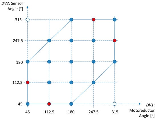
Figure 13.
Blue points represent the pairs of values of design variables (input parameters) created within DOE that correspond to possible combinations within the UGV assembly. White points were created within DOE but represent impossible combinations of parameter values. Red points represent the remaining possible combinations that were not covered by DOE.
From Figure 13, it is evident that 15 out of 19 possible combinations of design variables were covered by the DOE. Additionally, two impossible combinations of design variables were also included in DOE and served as the basis for two FEA simulations. Those simulations, though, yielded the results that were important for accurate construction of response surfaces. Table 2 displays the maximum stresses and minimum safety factors found in specific components of the UGV. Figure 14 illustrates the stress distribution across the assembly components of the UGV under the conditions that result in the highest stress within the assembly.
Table 2.
Maximum Von Mises stress values of the UGV assembly and frame and corresponding values of safety factors for various combinations of design variables values. Each FEA solution, or virtual experiment, is denoted as design point (DP) n, with n ranging from 1 to the total number of experiments in DOE. Solutions representing unattainable parameter combinations are highlighted in gray (DP12 and DP14). The solutions are arranged based on the maximal assembly stress value.
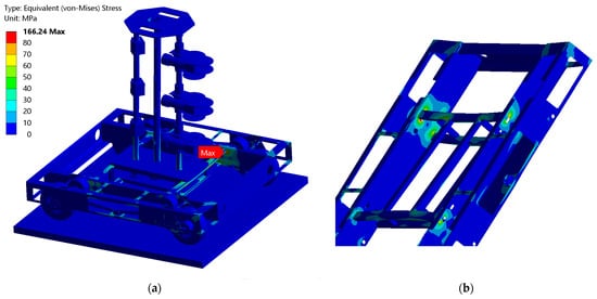
Figure 14.
Von Mises stress field corresponding to DP8 in Table 2: (a) UGV assembly, (b) frame.
Response surfaces of the “genetic aggregation” type were generated for all output parameters using the results of the DOE, as illustrated in Figure 15 and Figure 16.
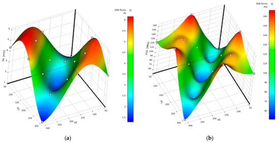
Figure 15.
(a) Response surface representing the maximum displacement value across the entire UGV assembly as a function of wire angles; (b) Response surface representing the maximum Von Mises stress value of the UGV frame as a function of wire angles.
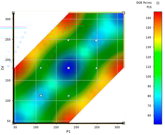
Figure 16.
Response surface representing maximum value of Von Mises stress of UGV frame as a function of wire angles. In this 2D view, surface regions corresponding to infeasible combinations of design variables were excluded.
The angle between wires originating from motoreductors and wires originating from sensors may be calculated as:
where αm is the angle denoted as “DV1: Motoreductor angle” in Figure 5 and αs is the angle denoted as “DV2: Sensor angle” in Figure 5.
By referring to Figure 16 and Table 2, it is evident that the greatest assembly stresses are present in scenarios associated with DP8, DP2, DP4, and DP6, all characterized by a 45° or 315° angle between the motoreductor and sensor wires. When an angle exceeds 180°, the explementary angle can be considered instead. In our case, the explementary angle of 315° equaled 360° − 315° = 45°, making all angles at which maximal stress is highest equal to 45°. Additionally, the data from Figure 16 and Table 2 reveal that the lowest stresses occur at an angle between the motoreductor and sensor wires of 180°, while mid values of stress occur at an angle of 112.5°. These results can be explained logically. At an angle between wires equal to 45°, the resultant force acting on the vertical post is maximal, whereas at an angle of 180°, wire forces nearly cancel each other out. If the stressed at design points for which the resultant angle is 45° are mutually compared, it is observed that the highest values occur when the angle between the resultant force and the frame diagonal is minimal (DP8, DP2, DP4, and DP6). For those design points, a stress concentration at oval holes near the connection of the two small C-shaped profiles and one large rectangular profile is pronounced, as can be seen from the top left section of Figure 14b.
Regarding stress distribution, the majority of UGV components exhibited extensive areas of low stress, suggesting significant room for weight reduction. Certain subassemblies, like columns or wheel assemblies, consisted of standard elements that were either not suitable for alteration or needed to maintain their integrity for purposes such as interfacing with other components or keeping the dirt out. However, the frame was identified as a subassembly where a substantial amount of excess material could be removed from the oversized profiles. Building on the findings and analysis presented earlier, it was determined that the bulky profiles of the frame would be targeted for weight reduction, with topology optimization selected as the appropriate method for this purpose.
From Figure 15b and Figure 16, it is obvious that response surface peaks are very close to stress values at design points yielding the highest frame stress. This was verified using Ansys DesignXplorer through response surface optimization (RSO) employing the multiobjective genetic algorithm (MOGA) with the goal of maximizing frame stress. The optimization process identified three potential points with maximum stress (Table 3), exhibiting parameter values similar to DP2. With a very small margin of 0.1 MPa, DP2 shared the highest stress level with DP8, while DP4 and DP6 had only slightly lower values of maximum stress. This analysis further supported the decision that TO would be based on four indicated load cases, i.e., on four design points for which the frame stress was the highest. The frame stress values obtained by FEA for these specific design points were very close to each other and significantly greater than those of the other design points (see Table 2 for reference).
Table 3.
Candidates for the optimal solution of response surface optimization (RSO) aiming at maximum UGV frame stress.
3.2. Topology Optimization (TO)
The process of topology optimization (TO) was carried out by considering four specific load cases and utilizing substructuring, as illustrated in Figure 17. For each load case, a corresponding substructuring analysis was defined based on the FE model outlined in Section Models Used in Substructuring, with displacements transferred from the main FE model (depicted in Figure 8a) to the submodel through cut boundary constraints (refer to Figure 11b). Following several preliminary TO runs, a fine and uniform mesh with an average edge size of 3.5 mm was created for further analyses (depicted in Figure 12). This choice was in line with prior experiences and recommendations from the software manufacturer, indicating that a fine mesh contributes to improved TO outcomes [23]. The selection of such a small edge size was beneficial as the thickness of rectangular profiles was only 3.8 mm, so the generated elements could stay proportional. Consequently, an FE mesh comprising 1,685,800 elements and 2,826,109 nodes was generated on the submodel.
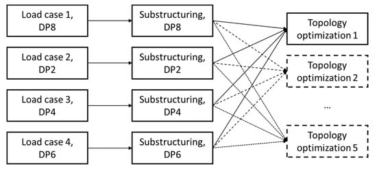
Figure 17.
TO workflow.
A comparison of von Mises stress distribution of the UGV frame obtained by FEA of the master model and submodel for load case 1 (DP8) is given in Figure 18, showing a very good match between the two. The difference in peak stress values was approximately 10% for all load cases, primarily due to employing a highly detailed mesh in the submodel.
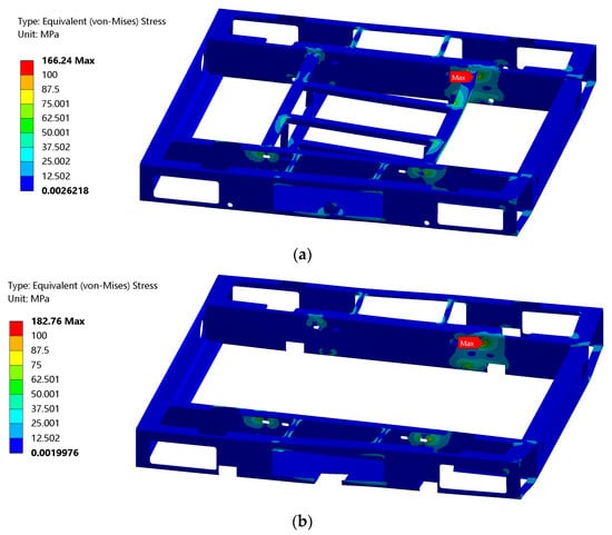
Figure 18.
Equivalent stress distribution of UGV frame obtained by FEA of (a) master model; (b) submodel.
Preliminary TO runs indicated that the mixable density method outperformed the density-based method in terms of boundary retention and shape integrity, while the level-set-based method did not yield a feasible solution. Consequently, the mixable density method was selected for further analysis. The definition of performed TO runs is shown in Figure 19. Four objectives were simultaneously set, each requiring the minimization of compliance (i.e., maximization of stiffness) in relation to one of the four load cases. All four profiles were designated as the design region, i.e., the region in which the TO may be performed. The cut boundaries were excluded from TO to ensure that the resulting geometry remained connected with the geometry containing the contact surfaces between the frame and other UGV components. Additionally, the inside plates of two rectangular profiles were omitted from TO as they served to protect the interior of the UGV from water and dirt ingress. Two design constraints were introduced to maintain the plane symmetry of the resulting geometry, defining symmetry about the XZ and YZ planes. The manufacturing constraints utilized in ANSYS 2023 R1 for TO include member size, pull-out direction, extrusion, AM overhang constraint, and housing [25]. Among these, only member size is applicable in the optimization of laser-cutting manufactured parts. This parameter determines the minimum thickness of geometric features, serving to prevent the generation of thin structures during TO. However, in ANSYS 2023 R1, it was not possible to use member size constraints with the mixable-density approach. Consequently, the manual avoidance of creating excessively thin features was necessary, as detailed in the subsequent sections. Five TO runs were defined, as depicted in Figure 17, with the response constraint ranging from 30% to 70% retained mass in 10% increments.
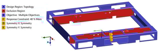
Figure 19.
Constraints and exclusion regions used in TO. Label “B” is not visible on the model but only in the legend. Nevertheless, it refers to the whole design region.
The outcomes of the five TO runs were examined, adjusting the “retained threshold” value to alter the percentage of material removed from the optimization region in each TO solution. The most suitable solution for modifying the frame geometry, as depicted in Figure 20, was achieved using a response constraint of 30% mass retention and a retained threshold value of 0.1, leading to a 34.6% mass retention. This solution served as the primary reference for frame geometry adjustments.
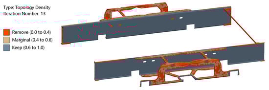
Figure 20.
The result of TO run with a response constraint of 30% mass retainment and retained threshold value of 0.1.
In the previous solution, a large portion of the frame that was still important for UGV integrity, robustness, and mounting of electronic components, such as fans, was omitted. Consequently, an additional TO solution (Figure 21), obtained with a 40% mass retention response constraint and retained threshold value of 0.1, was used to define the remaining portion of the frame.
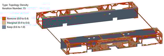
Figure 21.
The result of TO run with a response constraint of 40% mass retainment and retained threshold value of 0.1.
The optimized shape generated through TO, shown in Figure 20, was exported as a polygonal model to an STL file, and then imported into SolidWorks 2023. There, it was overlaid onto the current frame geometry to serve as a guide for trimming the central sections of rectangular profiles. The remaining regions of the frame were then reduced to slender sections defining its edges, similar to the geometry shown in Figure 21 but without intricate organic shapes that were challenging to replicate through cutting. The resultant frame geometry is displayed in Figure 22.

Figure 22.
Frame geometry obtained by the creation of additional cuts, based on TO results.
The optimization process led to a 39.8% reduction in mass across the four profiles that were defined as the optimization region. Subsequently, the whole frame experienced a 30.7% decrease in mass, while the entire UGV assembly saw a 9.5% mass reduction.
3.3. Validation of the Optimized Model
To confirm the structural integrity of the optimized UGV design under designated loads while ensuring minimal changes in stiffness and keeping stresses within safe thresholds, RSA, elaborated in Section 3.1, was conducted using the revised FE model (depicted in Figure 23). A more refined mesh was applied to the frame components to account for the finer details generated after TO. This led to an FE model consisting of 1,002,390 nodes contained in 298,152 finite elements. All other parameters, such as material properties, loads, boundary conditions, parameter ranges, and DOE definitions, remained consistent with the previous RSA iteration.
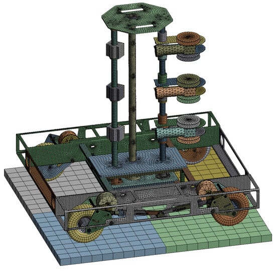
Figure 23.
The FE model of the UGV assembly with the frame modified based on TO results.
Maximum stresses and minimum safety factors of specific UGV components, obtained using the modified FE model, are shown in Table 4. The stress distribution across the assembly components of the UGV corresponding to the load case causing the highest stress within the assembly (DP2) is shown in Figure 24.
Table 4.
Maximum Von Mises stress values of the UGV assembly and frame and corresponding values of safety factors for various combinations of design variable values, obtained by FEA of the modified UGV model.
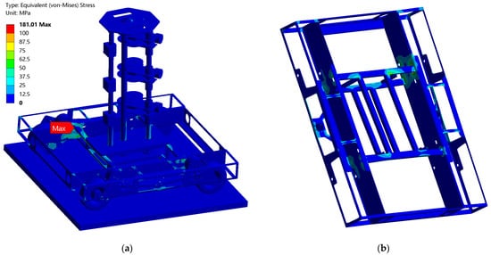
Figure 24.
Von Mises stress field corresponding to DP2 in Table 4: (a) UGV assembly, (b) frame.
Response surfaces of the “genetic aggregation” type generated during RSA based on the updated FE model are shown in Figure 25. The new surfaces were almost identical in shape to the ones obtained in the first RSA (refer to Figure 15).
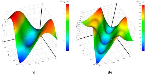
Figure 25.
Response surface generated using the modified UGV model: (a) Response surface representing the maximum displacement value across the entire UGV assembly as a function of wire angles; (b) Response surface representing the maximum Von Mises stress value of the UGV frame as a function of wire angles.
Upon comparing the results obtained during the RSA of the original and optimized models, it may be seen that, despite substantial mass reduction, the performance of UGV did not change significantly. The peak assembly stress, which coincided with the peak frame stress, was equal to 166.24 MPa (at DP8) and after optimization increased to 181.01 MPa (at DP2), representing a 9% rise. The corresponding safety factor decreased from 2.14 to 1.96, still maintaining a high value. The maximum displacement value, crucial for the proper functioning of winding coils and indicative of assembly stiffness, was 5.53 mm at DP5 and increased to 5.91 mm at DP15, reflecting a 6.9% change deemed insignificant for the proper functioning of the UGV unit. The significant resemblance in the response surfaces obtained before and after topology optimization indicates that the overall behavior of the UGV unit, when considering load directions leading to maximum displacement or stress, remained largely unchanged.
3.4. Buckling Analysis
To address any doubts regarding the potential buckling of slender components in the optimized UGV design, an RSA consisting of 17 nonlinear eigenvalue buckling analyses was performed. Each buckling analysis was performed according to the procedure described in [25], which aligns with the standard method for analyzing elastic buckling in textbooks. The analyses were based on the preceding static structural nonlinear prestress analyses, maintaining the load patterns used in those analyses. The first eight buckling load multipliers were computed in each analysis, with the results presented in Table 5. These multiplying load factors can be interpreted as buckling safety factors. With the lowest calculated load multiplier being 46.1 (DP8, load multiplier 6), it can be confidently stated that the UGV structure can withstand the designated loading conditions without buckling.
Table 5.
The values of load multipliers obtained by buckling analyses.
The buckling mode shape corresponding to the lowest obtained value of the load multiplier and the corresponding load case is shown in Figure 26.
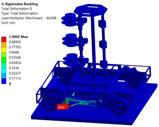
Figure 26.
The buckling mode shape corresponding to the lowest absolute load multiplier value of 46.1 (DP8, load multiplier 6).
3.5. Computational Resources and Analyses Times
The optimization was conducted on a standard engineering workstation featuring an Intel Core i9−12900KS processor running at 3.42 GHz and 128 GB of RAM. A typical FEA representing a single virtual experiment within the RSA took between 31 and 44 min. For four analyses involving a 180° angle between the motoreductor and sensor wires, durations ranged from 50 to 88 min. This variation in time was anticipated due to the increased time required to achieve static equilibrium when forces acted in opposite directions on the FE model featuring many contact surfaces. The cumulative duration of all FE analyses amounted to 12.4 h, while the total RSA time approached 14 h, accounting for additional time needed for parameter adjustments, CAD model regeneration, and new FE model creation. Substructuring analyses were completed in under 6 min each. TO using response constraints of 30% and 40% mass retainment took 2.5 and 2.8 h, respectively. The final RSA lasted around 16 h due to the inclusion of more finite elements in the corresponding FE model compared to the initial RSA. In total, 36 h of computational time were required to complete all phases of the optimization process. In addition, buckling RSA took around 18 h to complete.
The analysis times given above were considered completely acceptable in the context of project duration (two years) and when compared to the considerably longer model preparation times. Despite the majority of UGV components being thin walled, we concluded that there was no justification for employing shell elements. Although utilizing shell elements might likely accelerate the analyses, we considered that the accuracy of results in some model regions would be lowered. Additionally, the time saved as mentioned earlier could be negated as extra time would be required to model connections between shell and solid elements.
4. Discussion
In comparison to similar structural optimization studies centering on TO, e.g., [15,16,18,27,29], this study is innovative for its utilization of RSA in determining the worst load cases and the incorporation of submodels in TO. Additionally, the simultaneous consideration of multiple load cases, as demonstrated here, is seldom addressed in the existing literature. The complexity of the FE model utilized in this analysis surpasses that of typical models found in research, reflecting the unique design characteristics of the UGV which, to the best of our knowledge, have not been explored in the literature.
In addition to model complexity, another factor necessitated the use of substructuring. The complete UGV structure exhibited geometrically nonlinear behavior as a result of significant displacements of slender column structures, while the behavior of the frame could accurately be described as linear. Since the software utilized for TO could not handle nonlinear models, substructuring was essential, regardless of the model’s complexity.
The optimization process began with the prototype model, where the frame was constructed using standard profiles in which cuts were already created based on the need for accessing the wheel subassemblies and experience-based lightweighting. Having this in mind, the substantial 30.7% reduction in frame mass and 9.5% reduction in the overall UGV unit mass are regarded as significant achievements.
There is a strong likelihood that TO could yield better results if the initial design area was more extensive, consisting of profiles with minimal cuts essential for component mounting and structural maintenance. Based on the insights gained from this research, it is anticipated that in the future UGV design processes TO will be conducted at an earlier stage, beginning with bulk material regions, to enable the selection of optimal materials and shapes from the outset.
In summary, we consider that the methodology used enables the successful optimization of rather complex structures showing geometrically nonlinear behavior, particularly advantageous for rapid prototype development. One potential example of its application can be seen in agricultural robots with extended manipulator subassemblies. This is due to the potential existence of geometric nonlinearities and the significant impact of the manipulator’s position on structural loads. Those issues could be handled by adding RSO and substructuring to TO, similar to the procedure shown in this paper. We also consider that this approach applies not only to UGVs but also to any similar structures seeking lightweight design improvements. This could be particularly significant for UGVs and structures where payload capacity and weight are crucial factors. In essence, there appear to be no barriers to the applicability and scalability of this methodology.
The authors are considering using the methodology outlined in this study to optimize other machines that are currently under development or in the planning stages. For instance, the design of the earlier mentioned AgAR robot, which was previously optimized using TO only [10], could be revisited. Given the robot’s characteristics, such as adjustable ground clearance, wheel positioning, and platform leveling, RSA could be utilized to identify the most severe loading scenario. Additionally, by combining substructuring with TO, a more detailed design of its components could be achieved.
Author Contributions
Conceptualization, M.B. and N.K.; methodology, N.K. and M.B.; validation, N.K., V.P. and T.N.; formal analysis, N.K. and T.N.; investigation, N.K. and V.P.; writing—original draft preparation, N.K.; writing—review and editing, M.B., T.N. and V.P.; visualization, N.K. and V.P.; supervision, M.B.; project administration, M.B.; funding acquisition, M.B. All authors have read and agreed to the published version of the manuscript.
Funding
This research was funded in the frame of project RoboShepherd—automated animal husbandry and grazing system by the Innovation Fund of the Republic of Serbia and Coming Computer Engineering under grant number IF 50123.
Data Availability Statement
The data are not publicly available due to ownership by COMING.
Conflicts of Interest
The authors declare no conflicts of interest. The funders had no role in the design of the study; in the collection, analyses, or interpretation of data; in the writing of the manuscript; or in the decision to publish the results.
References
- Kondoyanni, M.; Loukatos, D.; Maraveas, C.; Drosos, C.; Arvanitis, K.G. Bio-inspired robots and structures toward fostering the modernization of agriculture. Biomimetics 2022, 7, 69. [Google Scholar] [CrossRef] [PubMed]
- Gangurde, Y.; Narayanan, S.S.; Rajalakshmi, P.; Mannam, N.P.B. Design of Autonomous Unmanned Ground Vehicles (UGVs) in Smart Agriculture. In Predictive Analytics in Smart Agriculture; CRC Press: Boca Raton, FL, USA, 2023; pp. 275–298. [Google Scholar]
- King, A.J.; Portugal, S.J.; Strömbom, D.; Mann, R.P.; Carrillo, J.A.; Kalise, D.; de Croon, G.; Barnett, H.; Scerri, P.; Groß, R. Biologically inspired herding of animal groups by robots. Methods Ecol. Evol. 2023, 14, 478–486. [Google Scholar] [CrossRef]
- Li, X.; Huang, H.; Savkin, A.; Zhang, J. Robotic Herding of Farm Animals Using a Network of Barking Aerial Drones. Drones 2022, 6, 29. [Google Scholar] [CrossRef]
- Karnovsky, I.A.; Lebed, O. Advanced Methods of Structural Analysis; Springer Nature: Berlin/Heidelberg, Germany, 2021. [Google Scholar]
- Christensen, P.W.; Klarbring, A. An Introduction to Structural Optimization; Springer Science & Business Media: Berlin/Heidelberg, Germany, 2008; Volume 153. [Google Scholar]
- Deaton, J.D.; Grandhi, R.V. A survey of structural and multidisciplinary continuum topology optimization: Post 2000. Struct. Multidiscip. Optim. 2014, 49, 1–38. [Google Scholar] [CrossRef]
- Tyflopoulos, E.; Steinert, M. Topology and parametric optimization-based design processes for lightweight structures. Appl. Sci. 2020, 10, 4496. [Google Scholar] [CrossRef]
- Cook, R.D. Concepts and Applications of Finite Element Analysis; John Wiley & Sons: Hoboken, NJ, USA, 2007. [Google Scholar]
- Banić, M.; Simonović, M.; Stojanović, L.; Rangelov, D.; Miltenović, A.; Perić, M. Digital twin based lightweighting of robot unmanned ground vehicles. Facta Univ. Ser. Autom. Control Robot. 2022, 1, 187–199. [Google Scholar] [CrossRef]
- Gadekar, A.; Fulsundar, S.; Deshmukh, P.; Aher, J.; Kataria, K.; Patel, V.; Barve, S. Rakshak: A modular unmanned ground vehicle for surveillance and logistics operations. Cogn. Robot. 2023, 3, 23–33. [Google Scholar] [CrossRef]
- Mohebbi, A.; Safaee, S.; Keshmiri, M.; Keshmiri, M.; Mohebbi, S. Design, simulation and manufacturing of a tracked surveillance unmanned ground vehicle. In Proceedings of the 2010 IEEE International Conference on Robotics and Biomimetics, Tianjin, China, 14–18 December 2010; pp. 1268–1275. [Google Scholar]
- Vardin, S.; Demircioğlu, P.; Böğrekci, İ. Development and implementation of an unmanned ground vehicle for off-road applications. Acta Tech. Napoc.-Ser. Appl. Math. Mech. Eng. 2022, 65, 1S. [Google Scholar]
- Wildman, R.; Gaynor, A. Topology optimization for robotics applications. In Robotic Systems and Autonomous Platforms; Elsevier: Amsterdam, The Netherlands, 2019; pp. 251–292. [Google Scholar]
- Demir, N.; Sucuoğlu, H.S.; Böğrekci, İ.; Demircioğlu, P. Topology optimization of mobile transportation robot. Int. J. 3d Print. Technol. Digit. Ind. 2021, 5, 210–219. [Google Scholar] [CrossRef]
- Sha, L.; Lin, A.; Zhao, X.; Kuang, S. A topology optimization method of robot lightweight design based on the finite element model of assembly and its applications. Sci. Prog. 2020, 103, 0036850420936482. [Google Scholar] [CrossRef] [PubMed]
- Kunpeng, N.; Dongbo, L.; Fei, H.; Yifei, T.; Kai, Z. Research on the structural optimization design of ER300 palletizing robot. Open Autom. Control Syst. J. 2015, 7, 1405–1414. [Google Scholar] [CrossRef]
- Junk, S.; Klerch, B.; Nasdala, L.; Hochberg, U. Topology optimization for additive manufacturing using a component of a humanoid robot. Procedia Cirp 2018, 70, 102–107. [Google Scholar] [CrossRef]
- Mantovani, S.; Barbieri, S.G.; Giacopini, M.; Croce, A.; Sola, A.; Bassoli, E. Synergy between topology optimization and additive manufacturing in the automotive field. Proc. Inst. Mech. Eng. Part B: J. Eng. Manuf. 2021, 235, 555–567. [Google Scholar] [CrossRef]
- Kato, J. Material Optimization of Fiber Reinforced Composites Applying a Damage Formulation; Institut für Baustatik und Baudynamik der Universit¨at Stuttgart: Stuttgart, Germany, 2010. [Google Scholar]
- Zhu, J.; Gao, T. Topology Optimization in Engineering Structure Design; Elsevier: Amsterdam, The Netherlands, 2016. [Google Scholar]
- Manfredi, L. Future trends. In Endorobotics; Elsevier: Amsterdam, The Netherlands, 2022; pp. 359–377. [Google Scholar]
- Trapp, M.; Nestorović, T. Non-gradient full waveform inversion approaches for exploration during mechanized tunneling applied to surrogate laboratory measurements. Tunn. Undergr. Space Technol. 2022, 120, 104252. [Google Scholar] [CrossRef]
- Nguyen, L.T.; Nestorović, T. Reconstructing disturbance zones ahead of the tunnel face by elastic waveform inversion supported by a parametric level-set representation. Soil Dyn. Earthq. Eng. 2018, 115, 606–621. [Google Scholar] [CrossRef]
- Ansys, I. Reference Guide, Release 2023R1; ANSYS Inc.: Canonsburg, PA, USA, 2023. [Google Scholar]
- Tyflopoulos, E.; Steinert, M. A comparative study of the application of different commercial software for topology optimization. Appl. Sci. 2022, 12, 611. [Google Scholar] [CrossRef]
- Ismail, A.Y.; Na, G.; Koo, B. Topology and response surface optimization of a bicycle crank arm with multiple load cases. Appl. Sci. 2020, 10, 2201. [Google Scholar] [CrossRef]
- Pavlović, V.D. Development and Control of an Intelligent Connection System Between Physically Connected Robots. Ph.D. Thesis, University of Niš, Faculty of Mechanical Engineering, Niš, Serbia, 2023. Available online: https://eteze.ni.ac.rs/application/showtheses?thesesId=8668 (accessed on 11 March 2024).
- Slavov, S.; Konsulova-Bakalova, M. Optimizing weight of housing elements of two-stage reducer by using the topology management optimization capabilities integrated in SOLIDWORKS: A case study. Machines 2019, 7, 9. [Google Scholar] [CrossRef]
Disclaimer/Publisher’s Note: The statements, opinions and data contained in all publications are solely those of the individual author(s) and contributor(s) and not of MDPI and/or the editor(s). MDPI and/or the editor(s) disclaim responsibility for any injury to people or property resulting from any ideas, methods, instructions or products referred to in the content. |
© 2024 by the authors. Licensee MDPI, Basel, Switzerland. This article is an open access article distributed under the terms and conditions of the Creative Commons Attribution (CC BY) license (https://creativecommons.org/licenses/by/4.0/).