Article

A Dynamic Pole Motion Approach for Control of Nonlinear Hybrid Soft Legs: A Preliminary Study

1
Department of Mechanical and Electrical Systems Engineering, Beijing Institute of Technology, Beijing 100081, China
2
Department of Mechanical Engineering, University of Saskatchewan, Saskatoon, SK S7N 4T9, Canada
*
Author to whom correspondence should be addressed.
Machines 2022, 10(10), 875; https://doi.org/10.3390/machines10100875
Submission received: 9 September 2022 / Revised: 19 September 2022 / Accepted: 26 September 2022 / Published: 28 September 2022
(This article belongs to the Special Issue Advances in Applied Mechatronics)

Abstract

:
Hybrid soft leg systems have been studied for advanced gaits of soft robots. However, it is challenging to analyze and control hybrid soft legs due to their nonlinearity. In this study, we adopted dynamic pole motion (DPM) to analyze stability of a nonlinear hybrid soft leg system with dynamic Routh’s stability criterion and to design a proper controller for the nonlinear system with an error-based adaptive controller (E-BAC). A typical hybrid soft leg system was taken as an example, as such a system can easily become unstable and needs a controller to get the system back to a stable state. Specifically, E-BAC was designed to control the unstable hybrid soft leg fast with a minimal overshoot. As a nonlinear controller, the implanted E-BAC in a feedback control system includes two dominant dynamic parameters: the dynamic position feedback K p e , t and the dynamic velocity feedback K v e , t . These parameters were properly selected, and the feedback was continuously varying as a function of system error e t , exhibiting an adaptive control behavior. The simulation shows that this approach for constructing an adaptive controller can yield a very fast response with no overshoot.

1. Introduction

Locomotion is an essential function of autonomous terrestrial robot systems, which carry out exploring, monitoring, and delivering tasks in complex and harsh environments. Although wheeled robots have been used in various engineering applications due to easy and simple steering operation, they face challenges on rugged and uneven terrains [1]. Legged terrestrial mobile robots are more versatile in the locomotory performance, and recently various bioinspired legged robots from animals and insects have been studied and developed in the form of two-legged (bipedal) [2,3], four-legged (quadrupedal) [4,5], six-legged (hexapedal) [6,7], and eight-legged (octopedal) [8,9] robots. It has been investigated that more legs on a robot yield superior stability to less legs on a robot during locomotion. Recently, with the new robotic concept, resilient robot [10,11,12,13], the more legs, the more resilient. Inspired by insects, hexapedal robots present the most efficient gaits, considering both stability and energy consumption [14].
A leg of a six-legged insect generally consists of five rigid segments (exoskeleton), coxa, trochanter, femur, tibia, and tarsus from proximal (toward the body) to distal (away from the body), connected by hinge joints, forming a sprawled posture [15], as illustrated in Figure 1a. Inspired from the five exoskeletons of the insect leg, a leg of a typical hexapedal robot includes three rigid links (coxa, fused trochanter and femur, and tibia without tarsus) with rotary joints, yielding multi-shape legs with three degrees of freedom (DOFs) [16], as shown in Figure 1b. Recent interests in bionic soft robots have attracted much attention with advantages of sustaining large deformation, safe interaction, and flexibility of motions with higher DOFs. However, soft robots require high computational costs of control due to the high DOFs [17,18,19,20]. Alternatively, hybrid soft robots have been introduced with the combination of rigid and soft components of a robot based on the hybridization engineering principle [21,22,23,24], and thus the hybrid soft robots retain the advantages of both rigid and soft robots, such as easier control, lighter weight, more flexibility, and so on [25]. Moreover, additive manufacturing (i.e., 3D printing technology) has promoted the fabrication processes of hybrid soft robots with various stiffnesses of robotic components [26,27]. Recently, Jiang et al. [28] introduced the flexoskeleton (external skeleton with flexible joint) printing process, and they introduced flexoskeleton legs (a quadrupedal robot) to promote the gait of insect-inspired hybrid soft robots with flexible locomotory performance. For a more stable gait of the robot, a hexapedal hybrid soft robot is desired as illustrated in Figure 1c.
For accurate manipulations, positioning control is essential for robots. Compared to the conventional control of rigid robots, control of soft robots is laborious due to high or infinite DOFs, including bending and torsion (i.e., nonlinearity). Hybrid soft robots face similar complications in control of undeniable flexible nonlinear components, although the structure of a hybrid soft robot is less distorting than a fully soft robot’s in motion. Moreover, various control strategies should be considered by actuator mechanisms of a soft robot or a hybrid soft robot, such as a fluidic-driven actuator, magnetic-driven actuator, tendon-driven (indirect-driven) actuator, and motor-driven (direct-driven) actuator [29].
Various control approaches for soft robots have been studied in forms of open-loop control and closed-loop control. Without specific sensors and feedback, open-loop control is adopted with more accurate analytical models from physical models. Thus, the deformation and the motion are well predicted for mobility of the robot. However, open-loop control faces many problems during the performance of soft robots due to the limited applications, and open-loop control is suitable for simple actuation control [30,31,32]. Closed-loop control can achieve more accurate and robust actuation control of soft robots with flexible proprioceptive sensors to achieve autonomous controls. Adaptive control schemes have been applied for nonlinear systems, such as inverse optimal controllers [33,34], and the scope of the adaptive controls has been extended to soft robotics [35,36]. Other closed-loop control approaches have also been studied, such as PD or PID controls [37,38,39] and FEM-based controls [40,41,42]. However, those approaches have not completely been solutions of nonlinearity soft robots exhibit owing to large deformations.
Furthermore, intelligent control approaches, such as machine learning algorithms, have been introduced to soft robotics due to uncertainties encountered during modelling. Learning based-approaches can achieve model-free control strategies based on collected data from a soft robot’s motion [43,44,45,46]. In addition, unsupervised learning schemes to control soft robots are available [47,48]. Although intelligent control approaches can handle nonlinearities of a soft robot system, there is still limitations in applicability due to required large amounts of data for training. Significant time is required to collect sufficient data to use, and the quality of the collected data is not fully reliable [49].
In this study, we adopt a dynamic pole motion (DPM) approach to analyze a nonlinear time-variant hybrid soft leg system by dynamic Routh’s stability criterion and to control the system by an error-based adaptive controller (E-BAC). Applying DPM, the dynamic Routh’s stability criterion quickly determines the stability of a nonlinear system, while conventional stability analysis requires complex procedures for nonlinear systems. Moreover, E-BAC manipulates a system to operate fast with little or without overshoot for a stable and robust control by utilizing system error. We investigated the stability of the hybrid soft leg system by the dynamic Routh’s stability criterion, and discovered that the leg system retains multiple regions of stability and instability. In order to overcome the unstable regions, we designed and implanted E-BAC in the system to achieve distinguished performance of the controlled system. The controlled system presented very fast settling time (~0.4 s) without overshoot, by adjusting system parameters, such as damping ratio varied from 0.35 to 1 and bandwidth from ~36 Hz to ~9 Hz.

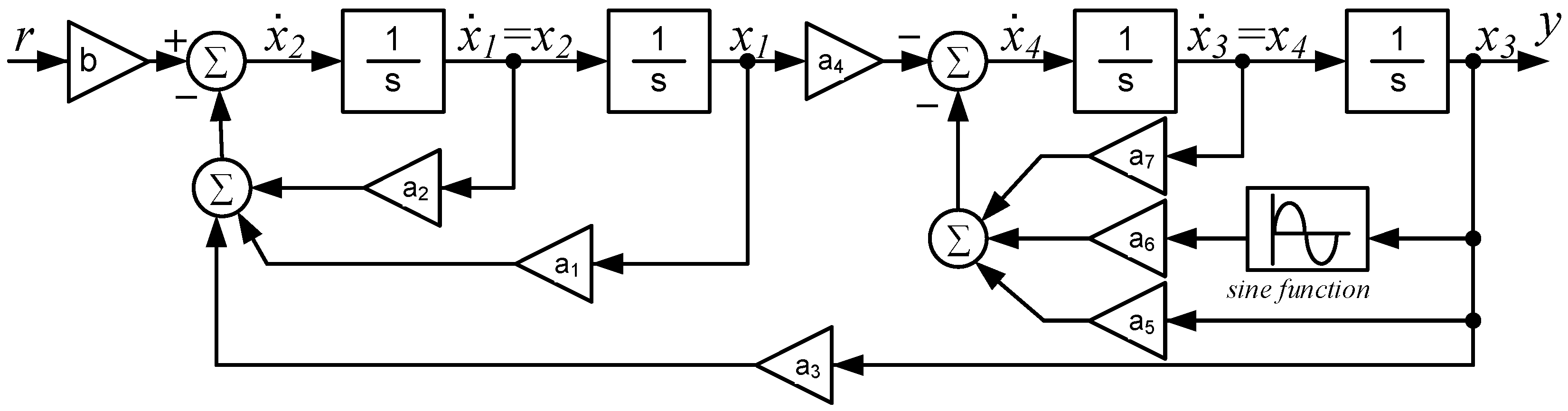
2. Analysis of a Motorized Hybrid Soft Leg: Dynamic Routh’s Stability Criterion for Nonlinear Systems

As illustrated in Figure 1, a leg of an insect, such as an ant, is composed of several connecting segments (called exoskeletons) as a structural support (i.e., link) or a joint. The exoskeletons are made from chitin networks which produce various stiffness (i.e., rigid or flexible) of the connecting exoskeletons depending on functions, dimensions, and shapes of the leg segments. The multi-stiffness of an insect leg significantly determines motions and mobility of an insect [28,50]. The rigid and flexible structure of an insect leg has motivated biomimetic hybrid soft legs, but the combination of various stiffness produces nonlinearity of the hybrid soft leg. A nonlinear system is simply described as a system whose output change is not proportional to input change, and a system is called as a time-variant system if the output of a system is varying depending on a function of time. Thus, nonlinear time-variant (NLTV) systems, such as soft robots (both complete and hybrid ones), are very challenging and difficult to be handled.
A hybrid soft leg can be schematically described with links and springs actuated by motors and gears as illustrated in Figure 2. A conventional 3D printing with polylactic acid (PLA) and thermoplastic polyurethane (TPU) could achieve the rigid link and the soft joint, respectively. The leg is connected through a gear train (harmonic drive) with the ratio n to a rigid link with length l, mass m, and moment of inertia m l 2 / 3 . The components of the structure are an actuator with rotor inertia JM, an actuator with viscous damping M, a joint actuator with a relative angular displacement θM, a motor shaft with a torque τM, and an end effector with a relative displacement θL. The joint flexibility is modeled by a linear torsional spring with stiffness k. Defining τM = r, the Euler–Lagrange equation can represent the dynamics of the hybrid soft leg as
m l 2 3 θ ¨ L + B L θ L ˙ + m g l 2 s i n θ L + k θ L + θ M n = 0
J M θ ¨ M + B M θ ˙ M + k n θ L + θ M n = r
Furthermore, defining x 1 t = θ M , x 2 t = θ ˙ M , x 3 t = θ L and x 4 t = θ ˙ L , the state variables xi, (i = 1, 2, 3, 4) can be derived as
x ˙ 1 t = x 2 t x ˙ 2 t = a 1 x 1 t a 2 x 2 t a 3 x 3 t + b r t x ˙ 3 t = x 4 x ˙ 4 t = a 4 x 1 t a 5 x 3 t a 6 s i n x 3 t a 7 x 4 t
where
b = 1 J M , a 1 = k J M n 2 , a 2 = B M J M , a 3 = k J M n a 4 = 3 k m n l 2 , a 5 = 3 k m l 2 , a 6 = 3 g 2 l , a 7 = 3 B L m l 2
From a block diagram of the motorized hybrid soft leg (see Figure 3), it is easily pointed out that this hybrid soft leg is NLTV since the sine function in the feedback loop of the system causes nonlinearity in the system, and the state variable x is dependent on function of time t, which yields some problems in designing an effective controller. The nonlinearity should be examined for designing a proper controller and analyzing stability of the system. In this study, we apply dynamic Routh’s stability criterion [51] to analyze the stability of this nonlinear hybrid soft leg system. Dynamic Routh’s stability criterion has advantages to analyze NLTV systems due to its simplicity as Routh’s stability criterion for linear time-invariant (LTI) systems.
The insight of dynamic Routh’s stability criterion was initiated by the perception that the position of poles and zeros of a system is changing (i.e., dynamic pole motion, DPM [52]) as the system state x varies with time t in a dynamic system. This rationale expanded the two-dimensional s-plane (i.e., real axis σ and imaginary axis ) to a three-dimensional g-plane (i.e., real axis σ, imaginary axis , and time-dependent variable) as illustrated in Figure 4. The stability region in the g-plane is defined from the definition of stability region in the s-plane (see Figure 4).
For simplicity, we set the value of the parameters ai ( i 1 , 7 ) and b equal to 1 in Equation (3) as
x ˙ 1 t = x 2 t x ˙ 2 t = x 1 t x 2 t x 3 t + r t x ˙ 3 t = x 4 t x ˙ 4 t = x 1 t 1 s i n x 3 t x 3 t x 3 t x 4 t
We first formulate a dynamic characteristic equation of the system by det g I A x , t = 0 , where
A x , t = 0 1 0 0 1 1 1 0 0 0 0 1 1 0 1 + s i n x 3 x 3 1
Thus, the dynamic characteristic equation of the motorized hybrid soft leg is given as
g 4 t + 2 g 3 t + 3 + ψ t g 2 t + 2 + ψ t g t + ψ t = 0 , ψ t = s i n x 3 t x 3 t .
With the dynamic characteristic equation, the stability of the hybrid soft leg system can be analyzed through dynamic Routh’s array as
g 4 1 ψ + 3 ψ g 3 2 ψ + 2 0 g 2 ψ + 4 2 ψ 0 g 1 ψ 2 + 2 ψ + 8 ψ + 4 0 0 g 0 ψ 0 0
Investigating the dynamic Routh’s array and considering that the Routh’s criteria for LTI systems is a subset of the dynamic Routh’s stability criterion for NLTV systems, we obtain the following interpretation:
(a)
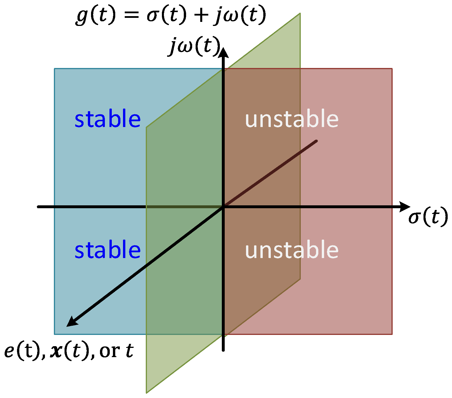
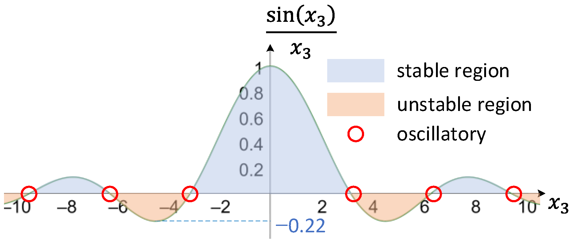
For stability of the system, all the elements in the first column of the dynamic Routh’s array must be positive non-zero values. Thus, we find that ψ > 0 from all the conditions of ψ + 4 > 0 , ψ 2 + 2 ψ + 8 > 0 , and ψ > 0 from each row, which means the condition of s i n x 3 t / x 3 t > 0 should be met to make the system stable. The stability region of s i n x 3 t / x 3 t is graphically represented in Figure 5.
(b)
Zero value at any rows in the first column of the dynamic Routh’s array represents that oscillatory dynamic poles are located on the imaginary axis of the g-plane, which indicates instability of the system. Zero value exists only if s i n x 3 t = 0 , which occurs periodically.
(c)
As the conventional Routh’s stability criterion, the dynamic Routh’s stability criterion can indicate the number of dynamic poles on the right-hand plane (RHP) of the g-plane by the number of sign (+ or −) changes in the first column of the dynamic Routh’s array. From the array, it can be found that one sign change could occur, which represents that one dynamic pole could be located in RHP of the g-plane when the system is not stable. Without a sign change, no dynamic poles are located in RHP of the g-plane, and the system is stable.
Next, the dynamic roots of this characteristic equation are calculated as
g 1 , 2 t = 1 2 1 ± 2 ψ 2 t + 4 2 ψ t 3 , g 3 , 4 t = 1 2 1 ± 2 ψ 2 t + 4 2 ψ t 3   .
The nonlinear function, ψ t = s i n x 3 t x 3 t , covers the range 0.22 ψ t 1 for all values of x 3 t over ,   , and the dynamic pole motion of this system is illustrated in Figure 6. As the system state x 3 t varies, the pole positions are fluctuating on the g-plane. Mostly, the poles are on the left-hand plane (LHP) in the g-plane, which represents stable states of the system. However, at some x 3 t values, one ( g 2 ) of the dynamic poles crosses over the imaginary axis to RHP, which implies unstable states of the system, and a proper controller is necessary for this hybrid soft leg.

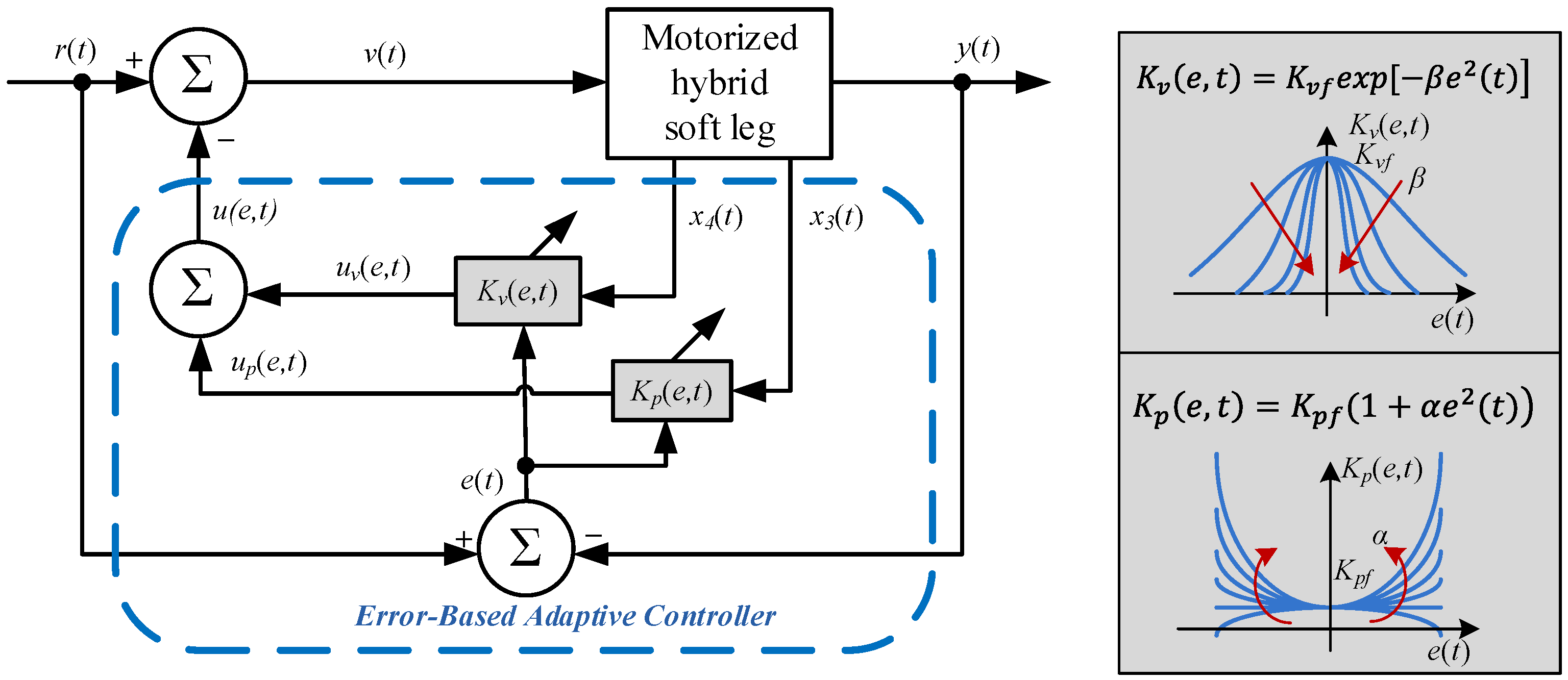
3. Error-Based Adaptive Controller (E-BAC) for the Motorized Hybrid Soft Leg

The initial concept of a dynamic pole motion (DPM) approach [52] was further standardized in [53,54] to facilitate the error-based adaptive controller (E-BAC) for nonlinear time-variant (NLTV) systems to accomplish a faster and more stable response of a system with little or without overshoots.
For the design of E-BAC, there are two dominant parameters to be considered, position feedback K p e , t and velocity feedback K v e , t . In a closed-loop control system, the feedback parameters are adapted by the system error e t and its states x t as shown in Figure 7, defining the position feedback K p e , t and the velocity feedback K v e , t gains as functions of system error e t [54] as
K p e , t = K p f 1 + α e 2 t
K v e , t = K v f e x p β e 2 t
e t = r t y t
y t = K p e , t x 1 t ,
where α and β are some gain constants which decide the slope of the functions and affect the system response, K p f and K v f are the final steady-state values of K p e , t and K v e , t , and e x p · is the exponential function as illustrated in Figure 7.
The position feedback K p e , t and the velocity feedback K v e , t gains were motivated from the natural frequency ( ω n ) and the damping ratio ( ζ ) of a conventional linear time-invariant (LTI) system. A small ζ and a large ω n (i.e., an underdamped dynamic with large bandwidth) yield a large error but a very fast system response with a very small rise time. Moreover, a large ζ and a small ω n (i.e., an overdamped system with a small bandwidth) result in a small error and inhibit overshoot of the system response. Therefore, defining K p e , t and K v e , t as functions of the system error, e t = r t y t , a very fast dynamic response of an NLTV system with no overshoot can be achieved. Designing K p e , t and K v e , t induces dynamic pole motions (DPM) (i.e., poles are moving as a function of time), and the system response can be controlled at an acceptable level following a linguistic algorithm [54] as below:
‘As error decreases from a large value to a small value, K p e , t = ω n 2 t is continuously decreased from a very large value to a small value, and simultaneously, K v e , t = 2 ζ t ω n t is increased from a small value to a large value’.
The error-based control signal u e , t is derived as a function of e t and time t using the following two steps:
p o s i t i o n   f e e d b a c k   c o n t r o l :   u p e , t = K p e , t x 3 t
v e l o c i t y   f e e d b a c k   c o n t r o l :   u v e , t = K v e , t x 4 t  
Thus, the total feedback signal u e , t is given by
u e , t = u p e , t + u v e , t ,
and, finally, the control signal v t (see Figure 4) is defined as
v t = r t u e , t
For this motorized hybrid soft leg, the design criteria of our error-based adaptive controller (E-BAC) follow some important points as below:
(a)
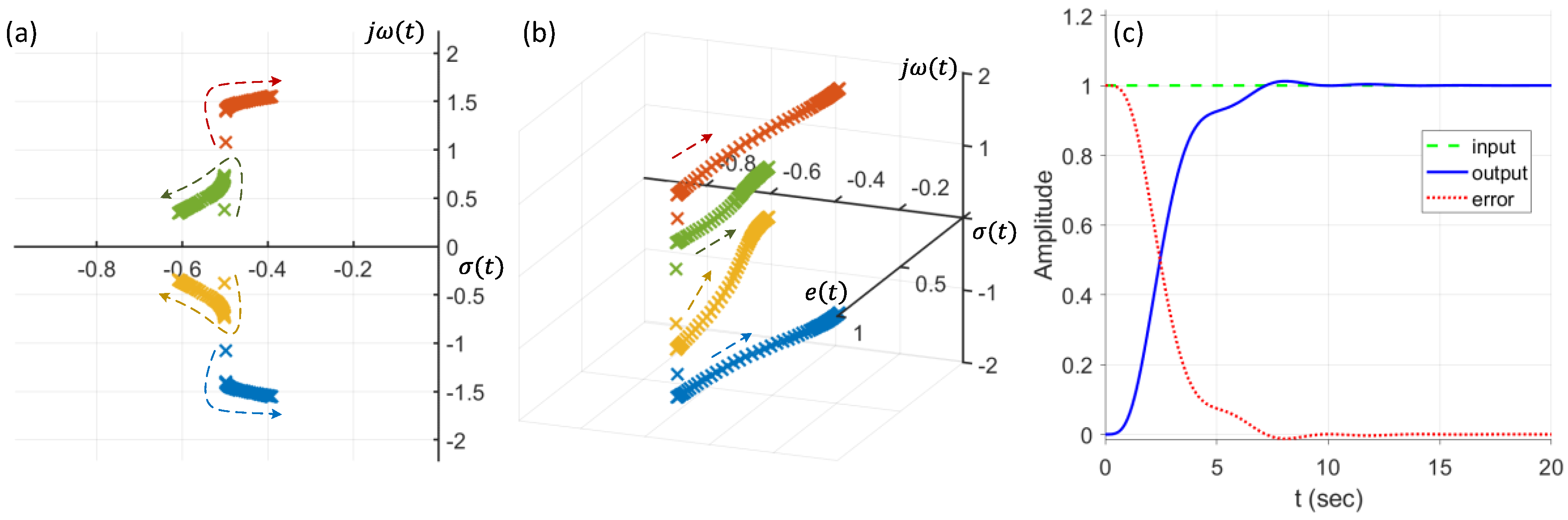
For the stability of the hybrid soft leg system, the dynamic poles should be always located on LHP on the g-plane for all values of x 3 t .
(b)
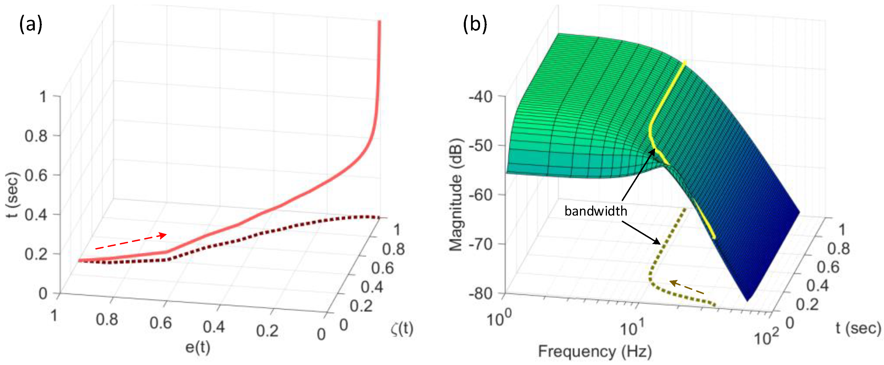
For achieving the fast response time, the system must have a large bandwidth for large errors and small bandwidth for small errors. Thus, the position feedback as the bandwidth parameter must be a function of the system error e t .
(c)
For no overshoot in the system response, damping should be adjusted continuously as a function of e t . K p e , t and K v e , t are designed such that they yield a small damping ratio with a large bandwidth for large errors, and a large damping ratio with small bandwidth for small errors.
The control input signal v t is derived as
v t = r t u e , t
u t = u p e , t + u v e , t
u p e , t = K p f 1 + α e 2 t   x 3 t
u v e , t = K v f e x p β e 2 t   x 4 t
where x 3 t = x and x 4 t = x ˙ are the states of the system, K p f and K v f are the steady-state values of feedback K p e , t and K v e , t , respectively, α and β are some gain constants for K p e , t and K v e , t , respectively, r t is the reference input of the system, and e t = y t r t =   r t K p e , t x 3 t is the system error.
As described in the design criteria, the objective of the embedded E-BAC is to design the control u t to make the system output y t follow the reference input signal r t . The dynamics of the close-loop system are continuously changing: initially for large errors, we make a large bandwidth and very small damping ratio ζ t , and as error decreases, the damping ratio ζ t is continuously increased, and the system bandwidth is decreased.

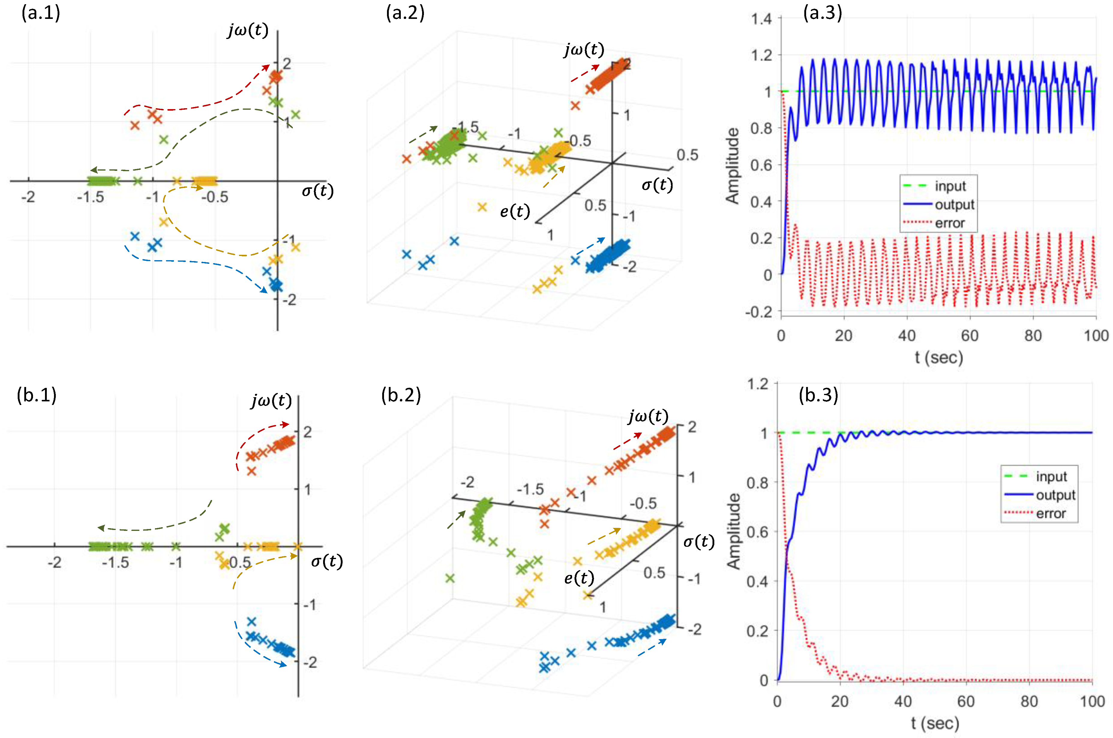
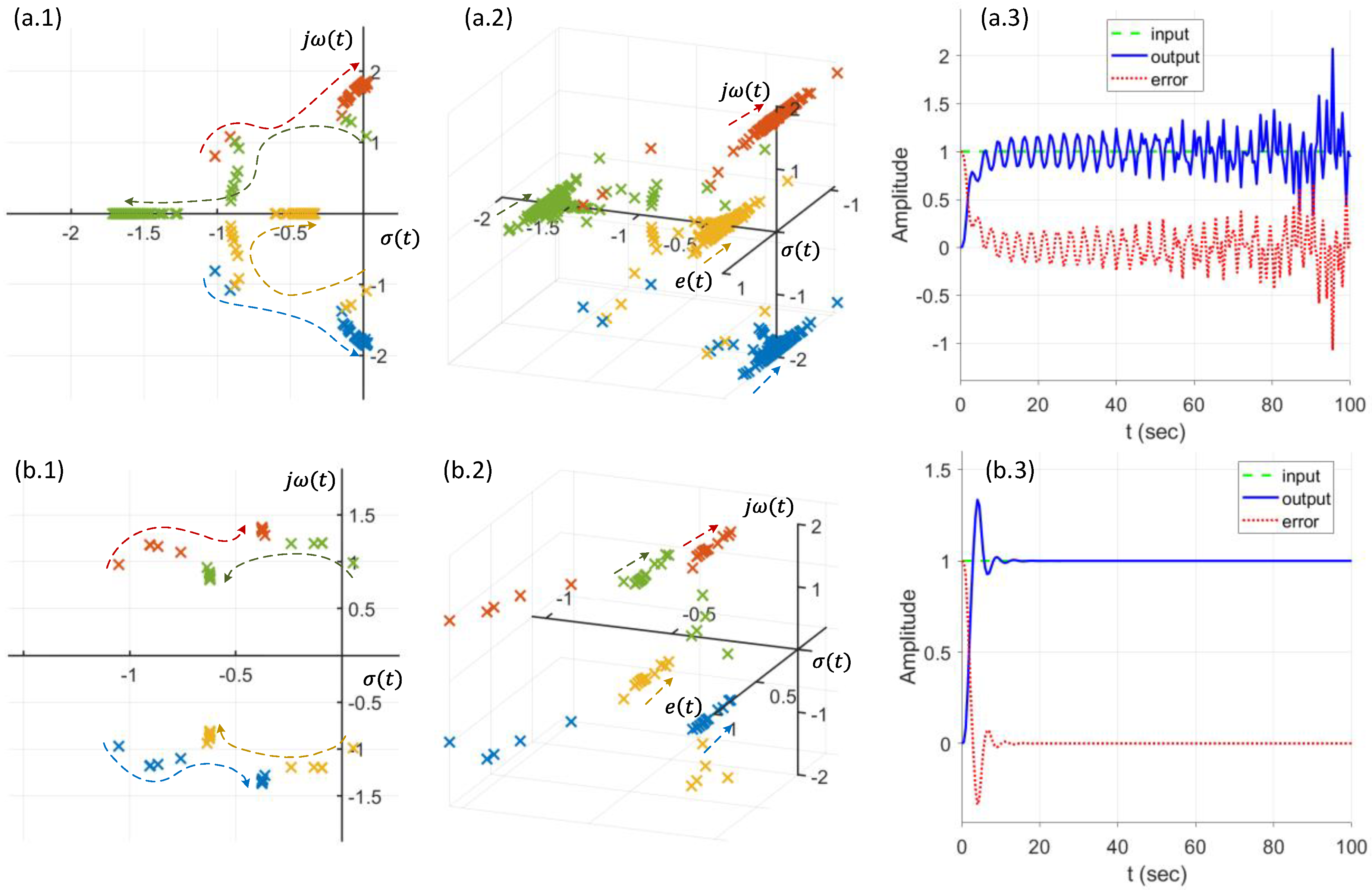
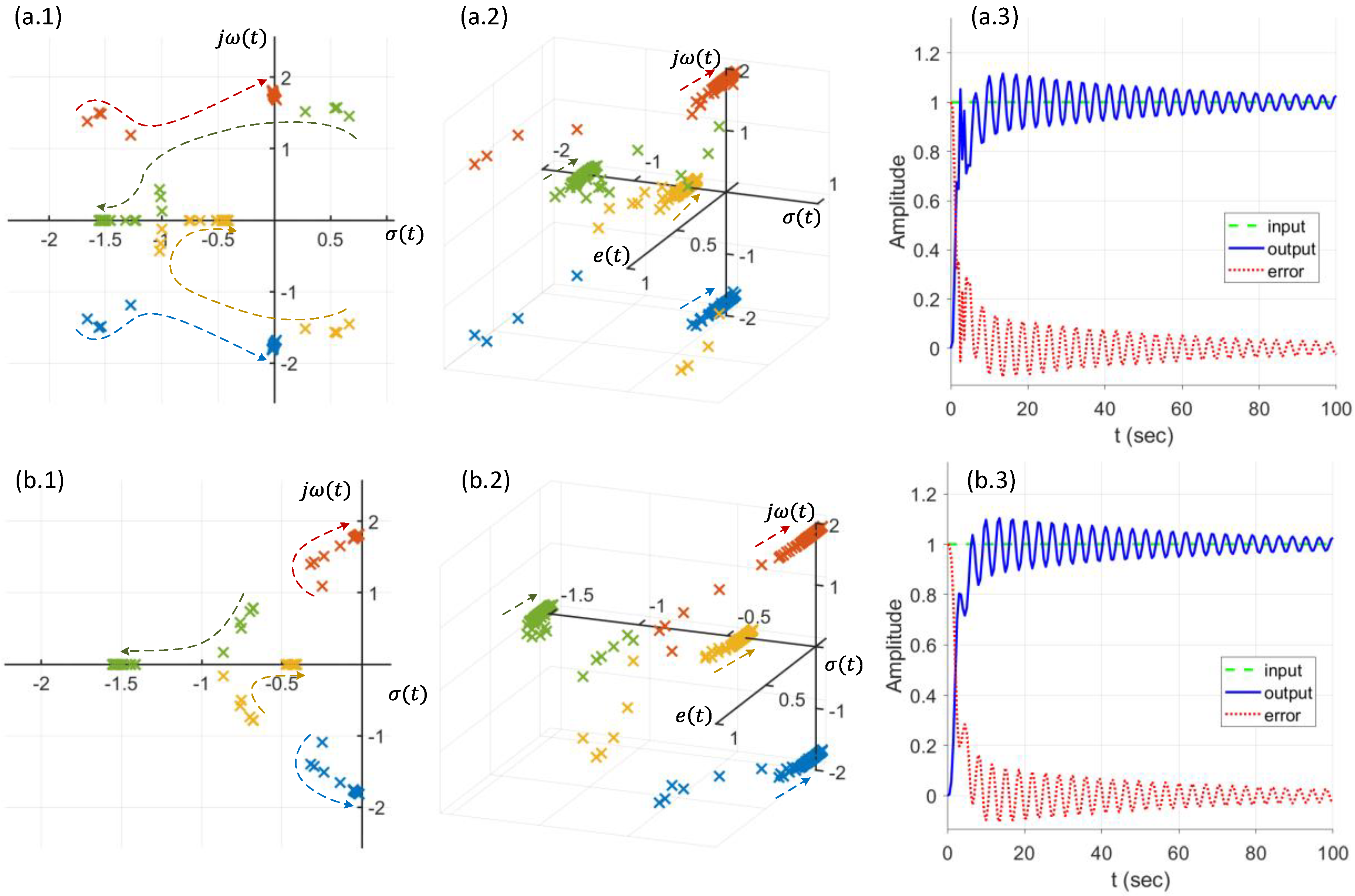
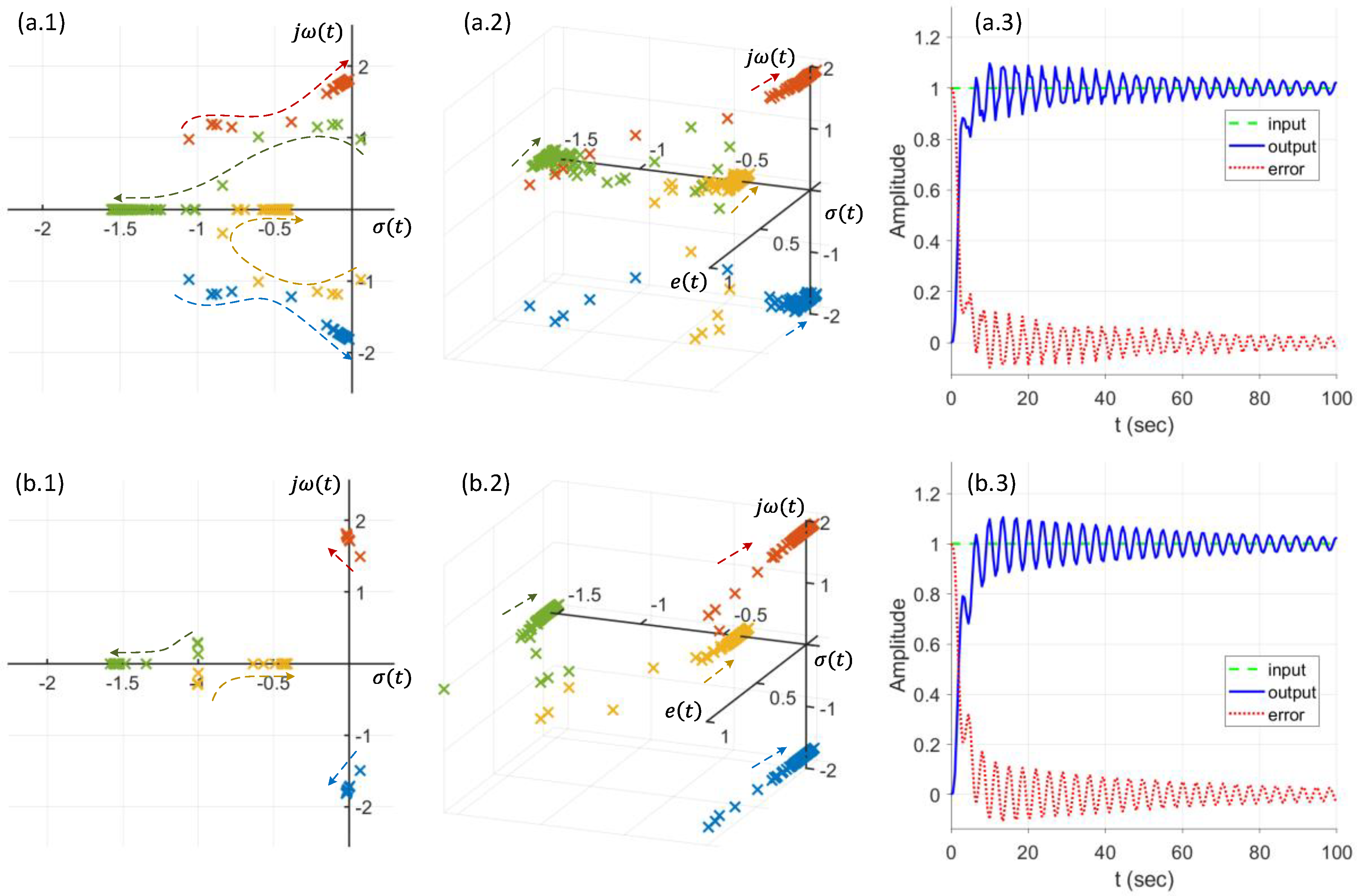
4. Simulation Study and Results

For a simulation study, we set the motorized hybrid soft leg in unstable states with x 3 t = 5 as indicated in the graphical representation (see Figure 5). In the design of the E-BAC, by the feedback K p e , t and K v e , t , the controlled system was expected to respond fast at the beginning (similar to an underdamped system) with large error, and then gradually the system was anticipated to behave slowly (as an overdamped system) with decreasing error. For the simulation, a step input ( r t = 1 ,   t > 0 ) was applied.
Initially, we arbitrarily chose the gains K p f = 1.1 , K v f = 3.5 , α = 1 , and β = 2 , and the results are shown in Figure 8. At t = 0 with an error of 1, two poles are placed in LHP (PLs), and the other two poles are located in RHP (PRs) near the imaginary axis. As time increased, the PLs approached the imaginary axis, and the PRs moved to the real axis in LHP with decreasing error. However, the changing error induced the oscillation of the system response by locating PRs near the imaginary axis (i.e., similar to an underdamped system). In the meantime, the error yielded the reduction of oscillation of the system by locating PLs on the real axis (i.e., similar to an overdamped system). Overall, the system response with the selected gains presented gradually decreasing oscillation to reach a stable state with reducing error. However, it took a long time (>100 s) before the system finally settled down.
Next, we investigated the gain to examine how the controlled system would behave by changing the individual gain values. First, we studied the effect of K p f on the controlled system response, keeping the initial values of other gains. K p f was initially set higher as K p f = 10 . With the increased K p f , the system response became unstable because PLs crossed the imaginary axis to the position in RHP after a certain time. A small increase of K p f = 1.5 yielded the system as stable, but the system response presented high oscillation with a small decrease, and thus the time to reach for a stable state (i.e., settling time) was longer (>500 s). However, lower gain, K p f = 0.1 , improved the system response as shown in Figure 9. All four poles were initially located in LHP, and as error changed, two poles approached near the imaginary axis, and the other two poles moved on the real axis in LHP (close to the origin). The error was reduced faster than that with a higher K p f , and the settling time with the small oscillation was also reduced because of the pole near the origin on the real axis. However, the settling time was still long (~50 s) with the small oscillation of the response before the settlement.
We further examined the effect of K v f on the controlled system response (i.e., only K v f was changed, keeping other gains with the initial values), and the results are exhibited in Figure 10. The initial poles with higher K v f   ( > ~ 4 ) were in both RHP (i.e., two PRs) and LHP (i.e., two PLs) similar to the case of higher K p f . As error changed, the PRs settled on the real axis in LHP, and the PLs moved to the imaginary axis and crossed the imaginary axis at higher K v f , which caused instability of the system. Lower K v f = 0.3 drove the controlled system stable and settled. As error changed, the two initial PRs moved to LHP, and the two initial PLs relocated toward the imaginary axis (but not close to it), which diminished the oscillation of the system. Moreover, the settling time was greatly reduced (~15 s). However, the controlled system presented a high overshoot as a typical underdamped system.
Next, only α was changed to investigate the effect on the controlled system response, keeping the other gains the initial values, and the controlled system responses are shown in Figure 11. Overall, both higher α = 10 (see Figure 11a) or lower α = 0.1 (see Figure 11b) did not significantly affect the system response, although the initial pole positions in both cases were different. The responses before and after altering α produced similar results with high oscillations and long settling time. Higher α drove the initial two PRs relatively further from the imaginary axis, and lower α induced all initial pole positions in LHP, but the final pole positions in both cases were similar (i.e., two poles near the imaginary axis, and two poles on real axis in LHP). The similar final pole positions induced similar system responses with high oscillation. However, the initial behaves of the controlled system became different with the different α values: higher α caused high peaks initially.
Finally, the effect of β was explored on the controlled system response with the initial values of other gains, and the results are presented in Figure 12. It was found that β did not also considerably influence the system response, but the initial system response and the shape of oscillation were slightly affected. Both higher and lower β induced two initial PRs and PLs, and the poles in both cases ended near the imaginary axis (two poles) and on the real axis (two poles) in LHP. The difference was that PRs settled on the real axis at higher β , but PLs landed on the real axis at lower β . As a result, lower β yielded smoother oscillating peaks, and higher β caused sharper oscillating peaks with lower error.
From the observation of the gain change, significances of gains in E-BAC to a control system were concluded as K p f and K v f mainly influence the oscillation of the system response, such as amplitude and decay, and α and β mostly affect the initial amplitude of the response and the shape of the oscillation. Considering the significance, we improved the controlled system response by selecting more proper gains as K p f = 0.25 , K v f = 0.5 , α = 2 , and β = 5 , and the results are presented in Figure 13. Small K p f and K v f produced little oscillation and its amplitude, and moderate α and β induced smooth curve of the controlled system response. Initially, all poles were placed in LHP. As error changed, two poles moved towards the imaginary axis (not close to it), and the other two poles approached the real axis in LHP, which resulted in a stable controlled system response with improved settling time (~7 s) without overshoot.
It should be noted that there would be more choices of gains to achieve the similar response as shown in Figure 13, but the settling time was not able to be greatly shortened (e.g., <1 s) because all four poles were dominant, and their movements for the system response were closely perturbed by each other’s. This explained that the current control system (simple structure and control design) of the motorized hybrid soft leg should be improved to keep two dominant system poles. In order to achieve two dominant poles of the control system, there will be various approaches to modify and/or to reform the physical structure with mechanical and electrical parts. In this study, we consider all the approaches as a compensator to add in the control system to achieve a compensated system ( G c ) of the motorized hybrid soft leg as illustrated in Figure 14. One of conceivable approaches for G c is to add two zeros near two poles not to disturb the movements of the other two dominant poles. In this study, we simply added zeros at −1 and −2 to achieve a G c as
G c t = g t + 1 g t + 2 g t + g 1 g t + g 2 g t + g 3 g t + g 4
We further set the gains of E-BAC as K p f = 210 , K v f = 31 , α = 2 , and β = 0.5 , and the controlled system response of the compensated motorized hybrid soft leg is shown in Figure 15. The selected gains placed initial positions of the dynamic poles of the system at g 1 , 2 0 = 0.99 and 1.99 , and g 3 , 4 0 = 8.76 ± j 23.6 . During the operation of the system, as error changed (to 0), the positions of the dynamic poles finally moved to −1, −1.93, −13.46, and −16.11 on the g-plane. The zeros located at around −1 and −2 by the compensator attracted two poles ( g 1 , 2 ) not to affect the dominant poles ( g 3 , 4 ). The controlled system response initially exhibited the trajectory of an underdamped system with a small damping ratio ( ζ t = 0.35 ) and a large bandwidth ( ω B W t = 35.62   H z ), and the response finally settled down like an overdamped system with a large damping ( ζ t = 1 ) and a smaller bandwidth ( ω B W t = 8.98   H z ). The settling time of the compensated system was extremely improved (~0.4 s), and no overshoot was observed.
It is clear from the figure that the dynamic motion of poles of the system is decided by the value of the system error. The initial positions of the dominant dynamic poles are placed to generate a low damping ratio ζ t and large bandwidth ω B W t of the system, which is the characteristic of an underdamped system. Thereafter, the dynamic poles are optimized and shifted as the system error decreases, increasing ζ t and reducing ω B W t . The final positions of the dominant dynamic poles drive the system as an overdamped system, resulting in large ζ t and small ω B W t . The variations of ζ t with respect to error and ω B W t at each time interval are shown in Figure 16.

5. Discussion and Conclusions

In this study, a new and simple control approach for NLTV hybrid soft leg system was introduced, employing the error-based adaptive controller (E-BAC) with the principle of dynamic pole motion (DPM). The design of this adaptive controller is conceptually error-based and can handle the complexity of the hybrid soft leg system. E-BAC is designed to continuously change feedback parameters as functions of the system error. Initially, the controller induces a large error to imitate an underdamped system with a small damping ratio and a large bandwidth, and then forces the system to behave as an overdamped system with a large damping ratio and a small bandwidth. In the state of an underdamped system, the system responds to the control signal quickly, and in the state of an over damped system, the system response becomes steady and stable to minimize (or eliminate) overshoots.
We first analyzed the motorized hybrid soft leg system by employing DPM and dynamic Routh’s stability criterion, and found that the system included three poles in LHP and one pole in RHP, which concluded that this system was genuinely unstable. We utilized E-BAC for the unstable system to achieve stable system performances. By selecting proper gain values of position and velocity feedback, the performance of the controlled system was improved and stable. However, it was still challenging to reduce the settling time and the overshoot of the controlled system.
Next, we enhanced the system response, especially the settling time and the overshoot, with a two-zero compensator to obtain a compensated system. A new E-BAC was designed for the compensated system where the motions of two dominant dynamic poles were not interrupted by other dynamic poles. As a result, the performance of the controlled system was greatly improved with very fast settling time (~0.4 s) without overshoot. During the processing, the damping ratio varied from 0.35 (t = 0) to 1 (t = ~0.4 s), but on the contrary, the bandwidth of the system changed from a large value (~36 Hz) to a small value (~9 Hz).
Several conclusions can be drawn from this study as follows:
The dynamic pole motion approach based on the g-plane is effective to control the NLTV hybrid soft leg systems.
The dynamic Routh’s stability criteria can quickly confirm the instability of the NLTV hybrid soft leg system.
The E-BAC can control an unstable state of the NLTV hybrid soft leg system to quickly get back to a stable state of the system without any overshoot.
On a general note, the approach to construct an error-based adaptive controller based on the concept of dynamic pole motion enjoys its simplicity to deal with the nonlinear dynamics of a plant, a hybrid soft let system in this case, especially quick settling time without overshoot. This approach thus has its merit over traditional control approaches. In the future, we will test this controller on a real hybrid soft leg system. Another future work is to apply this approach to constructing a controller for fully soft robotic systems, e.g., soft octopus [55], soft frog [56], and Jellyfish [57].

Author Contributions

Conceptualization, W.-J.Z. and K.-Y.S.; Methodology, W.-J.Z.; Software, K.-Y.S. and M.B.; Investigation, K.-Y.S.; Data Curation, K.-Y.S. and M.B.; Writing—Original Draft Preparation, K.-Y.S. and M.B.; Writing—Review and Editing, W.-J.Z.; Visualization, M.B. All authors have read and agreed to the published version of the manuscript.

Funding

This research received no external funding.

Data Availability Statement

Not applicable.

Conflicts of Interest

The authors declare no conflict of interest.

References

  1. Lu, Q.; Mahtab, B.; Zhao, F.; Song, K.Y.; Feng, Y. Bioinspiration to Robot Locomotion implementing 3D printed Foxtail Grass. In Proceedings of the 2021 IEEE International Conference on Robotics and Biomimetics (ROBIO), Sanya, China, 27–31 December 2021; pp. 69–73. [Google Scholar]
  2. Kim, D.; Jorgensen, S.J.; Lee, J.; Ahn, J.; Luo, J.; Sentis, L. Dynamic locomotion for passive-ankle biped robots and humanoids using whole-body locomotion control. Int. J. Robot. Res. 2020, 39, 936–956. [Google Scholar] [CrossRef]
  3. Wu, Q.; Yang, X.; Wu, Y.; Zhou, Z.; Wang, J.; Zhang, B.; Luo, Y.; Chepinskiy, S.A.; Zhilenkov, A.A. A novel underwater bipedal walking soft robot bio-inspired by the coconut octopus. Bioinspiration Biomim. 2021, 16, 046007. [Google Scholar] [CrossRef] [PubMed]
  4. Hyun, D.J.; Seok, S.O.; Lee, J.; Kim, S. High speed trot-running: Implementation of a hierarchical controller using proprioceptive impedance control on the MIT Cheetah. Int. J. Robot. Res. 2014, 33, 1417–1445. [Google Scholar] [CrossRef]
  5. Tanaka, H.; Chen, T.-Y.; Hosoda, K. Dynamic Turning of a Soft Quadruped Robot by Changing Phase Difference. Front. Robot. AI 2021, 8, 629523. [Google Scholar] [CrossRef] [PubMed]
  6. Yu, H.; Gao, H.; Ding, L.; Li, M.; Deng, Z.; Liu, G. Gait Generation with Smooth Transition Using CPG-Based Locomotion Control for Hexapod Walking Robot. IEEE Trans. Ind. Electron. 2016, 63, 5488–5500. [Google Scholar] [CrossRef]
  7. Fu, J.; Zhang, J.; She, Z.; Ovur, S.E.; Li, W.; Qi, W.; Su, H.; Ferrigno, G.; De Momi, E. Whole-body Spatial Teleoperation Control of a Hexapod Robot in Unstructured Environment. In Proceedings of the 2021 6th IEEE International Conference on Advanced Robotics and Mechatronics (ICARM), Chongqing, China, 3–5 July 2021; pp. 93–98. [Google Scholar]
  8. Grzelczyk, D.; Szymanowska, O.; Awrejcewicz, J. Kinematic and dynamic simulation of an octopod robot controlled by different central pattern generators. Proc. Inst. Mech. Eng. Part I: J. Syst. Control. Eng. 2019, 233, 400–417. [Google Scholar] [CrossRef]
  9. Kumar, V.A.; Meenakshipriya, B.; Bijoy Antony, P.T.; Adithya, B.; Vikinesh, M.H. Design and Fabrication of Octopod for Survey and Rescue Operation. IOP Conf. Ser. Mater. Sci. Eng. 2021, 1055, 012021. [Google Scholar] [CrossRef]
  10. Wang, F.; Qian, Z.; Yan, Z.; Yuan, C.; Zhang, W. A Novel Resilient Robot: Kinematic Analysis and Experimentation. IEEE Access 2020, 8, 2885–2892. [Google Scholar] [CrossRef]
  11. Wang, Z.; Qian, Z.; Song, Z.; Liu, H.; Zhang, W.; Bi, Z. Instrumentation and self-repairing control for resilient multi-rotor aircrafts. Ind. Robot. Int. J. Robot. Res. Appl. 2019, 45, 647–656. [Google Scholar] [CrossRef]
  12. Zhang, T.; Zhang, W.; Gupta, M.M. Resilient Robots: Concept, Review, and Future Directions. Robotics 2017, 6, 22. [Google Scholar] [CrossRef] [Green Version]
  13. Sun, Z.H.; Yang, G.S.; Zhang, B.; Zhang, W.J. On the concept of the resilient machine. In Proceedings of the 2011 6th IEEE Conference on Industrial Electronics and Applications, Beijing, China, 21–23 June 2011; pp. 357–360. [Google Scholar]
  14. Manoonpong, P.; Patanè, L.; Xiong, X.; Brodoline, I.; Dupeyroux, J.; Viollet, S.; Arena, P.; Serres, J.R. Insect-Inspired Robots: Bridging Biological and Artificial Systems. Sensors 2021, 21, 7609. [Google Scholar] [CrossRef] [PubMed]
  15. Chen, J.; Liang, Z.; Zhu, Y.; Zhao, J. Improving Kinematic Flexibility and Walking Performance of a Six-legged Robot by Rationally Designing Leg Morphology. J. Bionic Eng. 2019, 16, 608–620. [Google Scholar] [CrossRef]
  16. Weihmann, T. Survey of biomechanical aspects of arthropod terrestrialisation—Substrate bound legged locomotion. Arthropod Struct. Dev. 2020, 59, 100983. [Google Scholar] [CrossRef] [PubMed]
  17. Yang, H.; Xu, M.; Li, W.; Zhang, S. Design and Implementation of a Soft Robotic Arm Driven by SMA Coils. IEEE Trans. Ind. Electron. 2018, 66, 6108–6116. [Google Scholar] [CrossRef]
  18. Zhou, D.; Zuo, W.; Tang, X.; Deng, J.; Liu, Y. A multi-motion bionic soft hexapod robot driven by self-sensing controlled twisted artificial muscles. Bioinspiration Biomim. 2021, 16, 045003. [Google Scholar] [CrossRef]
  19. Chen, A.; Yin, R.; Cao, L.; Yuan, C.; Ding, H.K.; Zhang, W.J. Soft robotics: Definition and research issues. In Proceedings of the 2017 24th International Conference on Mechatronics and Machine Vision in Practice (M2VIP), Auckland, New Zealand, 21–23 November 2017; pp. 366–370. [Google Scholar]
  20. Tony, A.; Rasouli, A.; Farahinia, A.; Wells, G.; Zhang, H.; Achenbach, S.; Yang, S.M.; Sun, W.; Zhang, W. Toward a Soft Microfluidic System: Concept and Preliminary Developments. In Proceedings of the 2021 27th International Conference on Mechatronics and Machine Vision in Practice (M2VIP), Shanghai, China, 26–28 November 2021; pp. 755–759. [Google Scholar]
  21. Cao, L.; Dolovich, A.T.; Chen, A.; Zhang, W. Topology optimization of efficient and strong hybrid compliant mechanisms using a mixed mesh of beams and flexure hinges with strength control. Mech. Mach. Theory 2018, 121, 213–227. [Google Scholar] [CrossRef]
  22. Cheng, L.; Lin, Y.; Hou, Z.-G.; Tan, M.; Huang, J.; Zhang, W.J. Adaptive Tracking Control of Hybrid Machines: A Closed-Chain Five-Bar Mechanism Case. IEEE/ASME Trans. Mechatron. 2011, 16, 1155–1163. [Google Scholar] [CrossRef]
  23. Zhang, W.J.; Ouyang, P.R.; Sun, Z.H. A novel hybridization design principle for intelligent mechatronics systems. In Proceedings of the Abstracts of the International Conference on Advanced Mechatronics: Toward Evolutionary Fusion of IT and Mechatronics: ICAM 2010.5, Toyonaka, Japan, 4–6 October 2010; pp. 67–74. [Google Scholar]
  24. Wang, K.; Yin, R.; Lu, Y.; Qiao, H.; Zhu, Q.; He, J.; Zhou, W.; Zhang, H.; Tang, T.; Zhang, W. Soft-hard hybrid covalent-network polymer sponges with super resilience, recoverable energy dissipation and fatigue resistance under large deformation. Mater. Sci. Eng. C 2021, 126, 112185. [Google Scholar] [CrossRef]
  25. Stokes, A.; Shepherd, R.; Morin, S.A.; Ilievski, F.; Whitesides, G.M. A Hybrid Combining Hard and Soft Robots. Soft Robot. 2014, 1, 70–74. [Google Scholar] [CrossRef]
  26. Stano, G.; Percoco, G. Additive manufacturing aimed to soft robots fabrication: A review. Extreme Mech. Lett. 2020, 42, 101079. [Google Scholar] [CrossRef]
  27. Sachyani Keneth, E.; Kamyshny, A.; Totaro, M.; Beccai, L.; Magdassi, S. 3D Printing Materials for Soft Robotics. Adv. Mater. 2021, 33, 2003387. [Google Scholar] [CrossRef] [PubMed]
  28. Jiang, M.; Zhou, Z.; Gravish, N. Flexoskeleton Printing Enables Versatile Fabrication of Hybrid Soft and Rigid Robots. Soft Robot. 2020, 7, 770–778. [Google Scholar] [CrossRef] [PubMed]
  29. Wang, J.; Chortos, A. Control Strategies for Soft Robot Systems. Adv. Intell. Syst. 2022, 4, 2100165. [Google Scholar] [CrossRef]
  30. Tolley, M.T.; Shepherd, R.F.; Mosadegh, B.; Galloway, K.C.; Wehner, M.; Karpelson, M.; Wood, R.J.; Whitesides, G.M. A Resilient, Untethered Soft Robot. Soft Robot. 2014, 1, 213–223. [Google Scholar] [CrossRef]
  31. Martinez, R.V.; Branch, J.L.; Fish, C.R.; Jin, L.; Shepherd, R.F.; Nunes, R.M.; Suo, Z.; Whitesides, G.M. Robotic Tentacles with Three-Dimensional Mobility Based on Flexible Elastomers. Adv. Mater. 2013, 25, 205–212. [Google Scholar] [CrossRef] [PubMed]
  32. Marchese, A.D.; Komorowski, K.; Onal, C.D.; Rus, D. Design and control of a soft and continuously deformable 2D robotic manipulation system. In Proceedings of the 2014 IEEE International Conference on Robotics and Automation (ICRA), Hong Kong, China, 31 May–7 June 2014; pp. 2189–2196. [Google Scholar]
  33. Sepulchre, R.; Jankovic, M.; Kokotovic, P.V. Integrator forwarding: A new recursive nonlinear robust design. Automatica 1997, 33, 979–984. [Google Scholar] [CrossRef]
  34. Kalman, R.E. When Is a Linear Control System Optimal? J. Basic Eng. 1964, 86, 51–60. [Google Scholar] [CrossRef]
  35. Skorina, E.H.; Luo, M.; Tao, W.; Chen, F.; Fu, J.; Onal, C.D. Adapting to Flexibility: Model Reference Adaptive Control of Soft Bending Actuators. IEEE Robot. Autom. Lett. 2017, 2, 964–970. [Google Scholar] [CrossRef]
  36. Cao, G.; Liu, Y.; Zhu, Z. Observer-based Adaptive Robust Control of Soft Pneumatic Network Actuators. Int. J. Control. Autom. Syst. 2022, 20, 1695–1705. [Google Scholar] [CrossRef]
  37. Gerboni, G.; Diodato, A.; Ciuti, G.; Cianchetti, M.; Menciassi, A. Feedback Control of Soft Robot Actuators via Commercial Flex Bend Sensors. IEEE/ASME Trans. Mechatron. 2017, 22, 1881–1888. [Google Scholar] [CrossRef]
  38. Li, D.; Dornadula, V.; Lin, K.; Wehner, M. Position Control for Soft Actuators, Next Steps toward Inherently Safe Interaction. Electronics 2021, 10, 1116. [Google Scholar] [CrossRef]
  39. Khan, A.H.; Shao, Z.; Li, S.; Wang, Q.; Guan, N. Which is the best PID variant for pneumatic soft robots an experimental study. IEEE/CAA J. Autom. Sin. 2020, 7, 451–460. [Google Scholar] [CrossRef]
  40. Katzschmann, R.K.; Thieffry, M.; Goury, O.; Kruszewski, A.; Guerra, T.-M.; Duriez, C.; Rus, D. Dynamically Closed-Loop Controlled Soft Robotic Arm using a Reduced Order Finite Element Model with State Observer. In Proceedings of the 2019 2nd IEEE International Conference on Soft Robotics (RoboSoft), Seoul, Korea, 14–18 April 2019; pp. 717–724. [Google Scholar] [CrossRef]
  41. Zhang, Z.; Dequidt, J.; Kruszewski, A.; Largilliere, F.; Duriez, C. Kinematic modeling and observer based control of soft robot using real-time Finite Element Method. In Proceedings of the 2016 IEEE/RSJ International Conference on Intelligent Robots and Systems (IROS), Daejeon, Korea, 9–14 October 2016; pp. 5509–5514. [Google Scholar] [CrossRef]
  42. Marchese, A.D.; Tedrake, R.; Rus, D. Dynamics and trajectory optimization for a soft spatial fluidic elastomer manipulator. In Proceedings of the 2015 IEEE International Conference on Robotics and Automation (ICRA), Seattle, WA, USA, 26–30 May 2015; pp. 2528–2535. [Google Scholar]
  43. Van Meerbeek, I.M.; De Sa, C.M.; Shepherd, R.F. Soft optoelectronic sensory foams with proprioception. Sci. Robot. 2018, 3, eaau2489. [Google Scholar] [CrossRef] [PubMed]
  44. Homberg, B.S.; Katzschmann, R.K.; Dogar, M.R.; Rus, D. Robust proprioceptive grasping with a soft robot hand. Auton. Robot. 2019, 43, 681–696. [Google Scholar] [CrossRef]
  45. Truby, R.L.; Della Santina, C.; Rus, D. Distributed Proprioception of 3D Configuration in Soft, Sensorized Robots via Deep Learning. IEEE Robot. Autom. Lett. 2020, 5, 3299–3306. [Google Scholar] [CrossRef]
  46. Kang, B.B.; Kim, D.; Choi, H.; Jeong, U.; Kim, K.B.; Jo, S.; Cho, K.-J. Learning-Based Fingertip Force Estimation for Soft Wearable Hand Robot With Tendon-Sheath Mechanism. IEEE Robot. Autom. Lett. 2020, 5, 946–953. [Google Scholar] [CrossRef]
  47. Glauser, O.; Wu, S.; Panozzo, D.; Hilliges, O.; Sorkine-Hornung, O. Interactive hand pose estimation using a stretch-sensing soft glove. ACM Trans. Graph. 2019, 38, 1–15. [Google Scholar] [CrossRef]
  48. Roberge, J.P.; Rispal, S.; Wong, T.; Duchaine, V. Unsupervised feature learning for classifying dynamic tactile events using sparse coding. In Proceedings of the 2016 IEEE International Conference on Robotics and Automation (ICRA), Stockholm, Sweden, 16–21 May 2016; pp. 2675–2681. [Google Scholar]
  49. Kim, D.; Kim, S.H.; Kim, T.; Kang, B.B.; Lee, M.; Park, W.; Ku, S.; Kim, D.; Kwon, J.; Lee, H.; et al. Review of machine learning methods in soft robotics. PLoS ONE 2021, 16, e0246102. [Google Scholar] [CrossRef] [PubMed]
  50. Clark, A.J.; Triblehorn, J.D. Mechanical properties of the cuticles of three cockroach species that differ in their wind-evoked escape behavior. PeerJ 2014, 2, e501. [Google Scholar] [CrossRef]
  51. Sahu, B.K.; Gupta, M.M.; Subudhi, B. Stability analysis of nonlinear systems using dynamic-Routh’s stability criterion: A new approach. In Proceedings of the 2013 International Conference on Advances in Computing, Communications and Informatics (ICACCI), Mysore, India, 22–25 August 2013; pp. 1765–1769. [Google Scholar]
  52. Song, K.; Gupta, M.M.; Jena, D.; Subudhi, B. Design of a robust neuro-controller for complex dynamic systems. In Proceedings of the NAFIPS 2009—2009 Annual Meeting of the North American Fuzzy Information Processing Society, Cincinnati, OH, USA, 14–17 June 2009; pp. 1–5. [Google Scholar]
  53. Song, K.-Y.; Gupta, M.M.; Jena, D. Design of an error-based robust adaptive controller. In Proceedings of the 2009 IEEE International Conference on Systems, Man and Cybernetics, San Antonio, TX, USA, 11–14 October 2009; pp. 2386–2390. [Google Scholar] [CrossRef]
  54. Song, K.-Y.; Gupta, M.M.; Homma, N. Design of an Error-Based Adaptive Controller for a Flexible Robot Arm Using Dynamic Pole Motion Approach. J. Robot. 2011, 2011, 726807. [Google Scholar] [CrossRef]
  55. Laschi, C.; Cianchetti, M.; Mazzolai, B.; Margheri, L.; Follador, M.; Dario, P. Soft Robot Arm Inspired by the Octopus. Adv. Robot. 2012, 26, 709–727. [Google Scholar] [CrossRef]
  56. Soomro, A.M.; Memon, F.H.; Lee, J.-W.; Ahmed, F.; Kim, K.H.; Kim, Y.S.; Choi, K.H. Fully 3D printed multi-material soft bio-inspired frog for underwater synchronous swimming. Int. J. Mech. Sci. 2021, 210, 106725. [Google Scholar] [CrossRef]
  57. Almubarak, Y.; Punnoose, M.; Maly, N.X.; Hamidi, A.; Tadesse, Y. KryptoJelly: A jellyfish robot with confined, adjust pre-stress, and easily replaceable shape memory alloy NiTi actuators. Smart Mater. Struct. 2020, 29, 075011. [Google Scholar] [CrossRef]
Figure 1. Comparison of six-legged insect and robot: (a) a biological six-legged ant and schematics of its hinder leg, (b) schematics of a rigid hexapedal robot and the structure of rigid leg with motors, and (c) schematics of a hybrid soft hexapedal robot and the structure of its hybrid soft leg with a motor and a spring. The same colors in 2D diagram represent the same segments of the leg (some segments in a biological insect leg are excluded in a robot leg). The blue arrow and the gray column at coxa joint in 2D diagram represent the direction of motion and the body, respectively.
Machines 10 00875 g001
Figure 2. A schematic diagram of the mechanism of a motorized hybrid soft leg illustrated in Figure 1c. The mechanical structure consists of a single link manipulator and a flexible spring joint.
Machines 10 00875 g002
Figure 3. Block diagram of the hybrid soft leg with rigid links and a flexible joint (spring). The system has both linear and nonlinear feedback.
Machines 10 00875 g003
Figure 4. Having the stability region, a three-dimensional g-plane consists of a real part σ t , imaginary part j ω t , and time-dependent part. The time-dependent part can be time t , error e t , or state variable x t .
Machines 10 00875 g004
Figure 5. Graphical representation of the stable region of the dynamic characteristic equation, g 4 t + 2 g 3 t + 3 + ψ t g 2 t + 2 + ψ t g t + ψ t = 0 . For simplicity of graphical representation, a specific time t is applied for ψ t .
Machines 10 00875 g005
Figure 6. The sketch of dynamic pole motion (DPM) of the hybrid soft leg without a controller: (a) two-dimensional representation with σ t - and j ω t -axes and (b) three-dimensional representation adding a x 3 t -axis. The arrows in (a) indicate the paths of pole movements.
Machines 10 00875 g006
Figure 7. Schematics of an error-based adaptive controller (E-BAC): x 4 t = x ˙ 3 t , and the change of the slopes of K p e , t and K v e , t curves. For various values of α and β, the directions of the arrows indicate the increasing values of α and β .
Machines 10 00875 g007
Figure 8. Dynamic pole motion of the controlled hybrid soft leg and the controlled system response by error change with the gains of K p f = 1.1 , K v f = 3.5 , α = 1 , and β = 2 : (a) 2D plot, (b) 3D plot, and (c) the system response to the step input. The arrows indicate the direction of pole motions.
Machines 10 00875 g008
Figure 9. Dynamic pole motions of the controlled hybrid soft leg and the controlled system response by error change with the gains of (a) K p f = 1.5 , K v f = 3.5 , α = 1 , and β = 2 , and (b) K p f = 0.1 , K v f = 3.5 , α = 1 , and β = 2 . The arrows indicate the direction of pole motions.
Machines 10 00875 g009
Figure 10. Dynamic pole motions of the controlled hybrid soft leg and the controlled system response by error change with the gains of (a) K p f = 1.5 , K v f = 4 , α = 1 , and β = 2 , and (b) K p f = 0.1 , K v f = 0.3 , α = 1 , and β = 2 . The arrows indicate the direction of pole motions.
Machines 10 00875 g010
Figure 11. Dynamic pole motions of the controlled hybrid soft leg and the controlled system response by error change with the gains of (a) K p f = 1.1 , K v f = 0.3 , α = 10 , and β = 2 , and (b) K p f = 1.1 , K v f = 0.3 , α = 0.1 , and β = 2 . The initial system responses were slightly distinct with different peaks, but the rest of the response remained similar. The arrows indicate the direction of pole motions.
Machines 10 00875 g011
Figure 12. Dynamic pole motions of the controlled hybrid soft leg and the controlled system response by error change with the gains of (a) K p f = 1.1 , K v f = 0.3 , α = 1 , and β = 20 , and (b) K p f = 1.1 , K v f = 0.3 , α = 1 , and β = 0.2 . The system responses were slightly distinct with different oscillating shapes (higher β presented sharper peaks), but the rest of the response remained similar. The arrows indicate the direction of pole motions.
Machines 10 00875 g012
Figure 13. Dynamic pole motion of the controlled hybrid soft leg and the controlled system response by error change with the gains of K p f = 0.25 , K v f = 0.5 , α = 2 , and β = 5 : (a) 2D plot, (b) 3D plot, and (c) the system response to the step input. The arrows indicate the direction of pole motions.
Machines 10 00875 g013
Figure 14. Schematic block diagram of a compensated system of the motorized hybrid soft leg with a compensator and E-BAC.
Machines 10 00875 g014
Figure 15. Dynamic pole motion of the controlled compensated hybrid soft leg and the system response by error change with the gains of K p f = 210 , K v f = 31 , α = 2 , and β = 0.5 : (a) 2D plot, (b) 3D plot, and (c) the system response to the step input ( ζ : damping ratio and ω B W : bandwidth in Hz). The arrows in (a,b) indicate the direction of pole motions.
Machines 10 00875 g015
Figure 16. Variations of properties of the controlled compensated system: (a) dynamic damping ratio ζ t (from 0.35 to 1) with respect to error and time (the dot line is the projection plot of ζ t on error-damping ratio plane), and (b) 3D sketch of dynamic magnitude plot of the system and dynamic bandwidth ω B W t (yellow curve, from 35.62 Hz to ~9 Hz) at each time interval (the dot line is the projection plot of ω B W t on frequency–time plane).
Machines 10 00875 g016
Publisher’s Note: MDPI stays neutral with regard to jurisdictional claims in published maps and institutional affiliations.

