Abstract
Cable-driven parallel robots (CDPRs) offer significant advantages, such as the lightweight design, large workspace, and easy reconfiguration, making them essential for various spatial applications and extreme environments. However, despite their benefits, CDPRs face challenges, notably the uncertainty in terms of the post-reconstruction parameters, complicating cable coordination and impeding mechanism parameter identification. This is especially notable in CDPRs with redundant constraints, leading to cable relaxation or breakage. To tackle this challenge, this paper introduces a novel approach using reinforcement learning to drive redundant constrained cable-driven robots with uncertain parameters. Kinematic and dynamic models are established and applied in simulations and practical experiments, creating a conducive training environment for reinforcement learning. With trained agents, the mechanism is driven across 100 randomly selected parameters, resulting in a distinct directional distribution of the trajectories. Notably, the rope tension corresponding to 98% of the trajectory points is within the specified tension range. Experiments are carried out on a physical cable-driven device utilizing trained intelligent agents. The results indicate that the rope tension remained within the specified range throughout the driving process, with the end platform successfully maneuvered in close proximity to the designated target point. The consistency between the simulation and experimental results validates the efficacy of reinforcement learning in driving unknown parameters in redundant constraint-driven robots. Furthermore, the method’s applicability extends to mechanisms with diverse configurations of redundant constraints, broadening its scope. Therefore, reinforcement learning emerges as a potent tool for acquiring motion data in cable-driven mechanisms with unknown parameters and redundant constraints, effectively aiding in the reconstruction process of such mechanisms.
1. Introduction
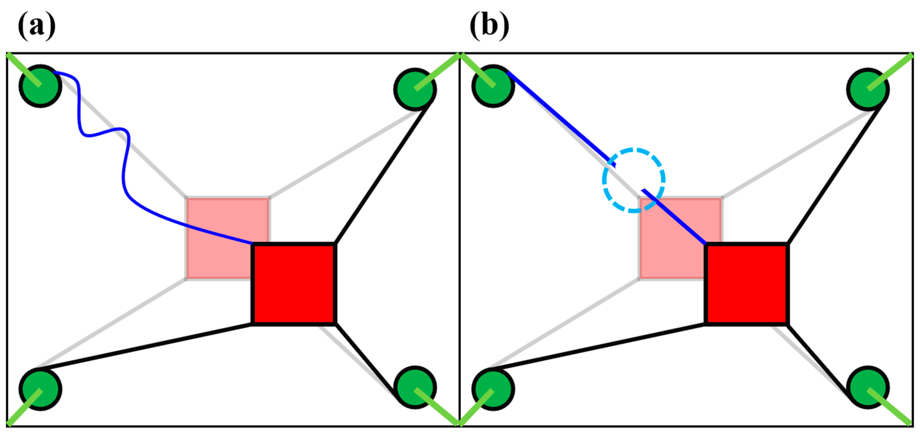
The cable-driven robot has garnered considerable attention from researchers owing to its impressive performance [1,2], which includes a high load-to-weight ratio, potential for a large forming space, high-speed motion, and ease of reconstruction [3,4,5,6,7,8]. Additionally, the cable-driven method offers significant flexibility compared to other drive mechanisms. It is widely employed in robots that require compliance and dexterity, such as multi-cable-driven continuum robots [9,10]. Particularly noteworthy is its ease of reconfiguration, which greatly facilitates equipment deployment in practical scenarios. In situations where robots are unable to be configured based on preset parameters due to terrain limitations or limited space, on-site parameter identification of the deployed equipment becomes crucial to ensure the robot’s accurate operation [11,12]. However, when dealing with unknown parameters, specific challenges arise in terms of parameter identification for cable-driven robots with redundant constraints. As depicted in Figure 1, when driving a cable-driven robot with redundant constraints and unknown parameters, ensuring the smooth and coordinated movement of multiple cables becomes challenging. This situation may lead to cables becoming loose or excessively tensioned. Loose cables can alter the mechanism’s behavior, rendering the acquired data unusable for the parameter identification of the original mechanism. Conversely, excessive tension in the cables can potentially damage the robot if protective measures are not in place or halt its movement if such measures are implemented. Both scenarios impede the acquisition of effective data for parameter identification, thereby complicating the process of discerning unknown parameters through the kinematic or dynamic characteristics of cable-driven robots.

Figure 1.
Explanation of the difficulty in driving a cable-driven mechanism with redundant constraints of unknown parameters. (a) The presence of unknown parameters presents a challenge to effectively coordinating and controlling the planar redundant constraint cable-driven mechanism, leading to cable relaxation. (b) The planar redundant constraint cable-driven mechanism, due to the presence of unknown parameters and the complexity of collaborative control, is susceptible to experiencing excessive tension in the cables, which can ultimately lead to cable fracture.
One method to address the aforementioned issue involves securing the end effector at various positions using auxiliary devices and employing precision instruments like laser rangefinders to gauge its position [13,14]. Subsequently, the length of each rope is iteratively adjusted until it is fully tensioned, just enough to maintain the end effector’s position upon removal of the auxiliary device. However, the complexity of the tension adjustment process makes this method time-consuming and labor-intensive.
Another approach entails optimizing or modifying the tension distribution of the ropes based on sensor data in response to instances of rope relaxation or excessive tension during the operation of the redundant constraint cable drive mechanism. The optimization of the tension distribution in CDPRs has garnered significant attention from researchers [15]. Geng X et al. [16] proposed the method of using two-dimensional polygons to determine a feasible set of rope forces, and then determining the optimal tension distribution based on various optimization objectives. Lim WB et al. [17] introduced the tension hypersphere mapping algorithm to avoid rope relaxation or excessive tension, avoid iterative calculations, and meet the requirements of real-time control design and trajectory planning. Furthermore, an enhanced gradient projection method has been utilized to derive adjustable tension solutions for each configuration, controllable via manipulation of the introduced tension-level index [18]. Another contribution involves the proposal of a real-time cable tension distribution algorithm for non-iterative two-degree-of-freedom redundancy CDPRs, addressing the imperative for real-time control in adjusting the cable tension for highly dynamic CDPRs [19].
While researchers have conducted numerous studies on optimizing the tension distribution of CDPRs, the proposed algorithm is not suitable for the specific issues outlined in this article. This limitation arises from the necessity when applying these methodologies of utilizing structural matrices, Jacobian matrices, or inverse kinematics of CDPRs, thereby requiring prior knowledge of the CDPRs’ parameters. Consequently, these control methods pose challenges when applied to adjusting the rope tension in CDPRs with unknown parameters.
Notable advancements in machine learning [20] have offered a promising avenue for addressing the challenge of the tension distribution in CDPRs with unknown parameters. This paper proposes the utilization of reinforcement learning to drive redundant-constrained CDPRs with unknown parameters. This novel method circumvents the issues of rope relaxation and excessive tension encountered during the operation of cable-driven robots with unknown driving parameters. Considering that the driving of CDPRs aims to collect data for parameter identification, the generated motion trajectory does not necessarily need to be accurate; rather, it should ensure that the rope tension remains within a specified range. Additionally, the generated trajectory should be distributed as evenly as possible throughout the workspace to ensure that the acquired data comprehensively reflect the characteristics of the mechanism, thereby enabling more accurate parameter identification.
At present, there is relatively little research on using machine-learning methods to study CDPRs. Xiong H et al. [21] proposed a control framework that combines robust controllers with a series of neural networks for controlling the direction of fully constrained cable-driven parallel robots with unknown Jacobian matrices. Piao J et al. [22] introduced a method for indirectly estimating end-effector forces using artificial neural networks to address the issue of inaccurate cable tension measurement, especially in CDPRs’ force control. Nomanfar P et al. [23] proposed using reinforcement learning to control cable-driven robots, which can avoid solving the complex dynamics of cable-driven robots. This study used reinforcement learning to control the motion of a rope-driven robot with a known configuration in a simulation environment. In order to solve the kinematics of CDPRs with cable wrapped on a rigid body, Xiong H et al. [24] developed a data-driven kinematic modeling and control strategy. This study indicates that data-driven kinematic modeling and control strategies can effectively control the CDPRs with cables wrapped around rigid bodies. Xu G et al. [25] developed a data-driven dynamic modeling strategy for a planar fully constrained rope driven robot that allows collision. This data-driven dynamic modeling strategy can simultaneously solve collision and optimal tension distribution problems. Zhang Z et al. [26] proposed using GNN to solve the forward kinematics (FK) problem of CDPRs. This study indicates that the proposed CafkNet can learn the internal topology information of CDPRs and act as an FK solver to accurately solve FK problems. A distinguishing feature of the present study when compared with prior research lies in the dynamic nature of the parameters under investigation. Existing research commonly addresses invariant parameters, whereas this study focuses on parameters that are both unknown and variable. Specifically, following each reconstruction, the parameters of the cable-driven robot are uncertain and distinct. Consequently, control methods derived through learning and training for a specific configuration are inapplicable. On the contrary, the agents trained through reinforcement learning in this paper can effectively drive any redundant-constrained CDPRs with unknown parameters, thus better meeting the real-time requirements of on-site operations.
The structure of this paper is organized as follows: Section 2 establishes the kinematic and dynamic models of the studied mechanism. Section 3.1 elaborates on the environmental setup for reinforcement learning utilizing the established dynamic model; Section 3.2 provides a concise introduction to the reinforcement learning Deep Deterministic Policy Gradient (DDPG) algorithm; and Section 3.3 discusses the methodologies for training and employing reinforcement learning agents. Section 4 presents the parameters for the computation and simulation, demonstrating the outcomes of the simulations and experiments. Section 5 examines the efficacy of extending the proposed method to various mechanisms. Finally, Section 6 provides the conclusion.
2. Kinematic and Dynamic Models
The subject of the investigation in this paper is a cable-driven parallel robot featuring redundant constraints, as depicted by way of an exemplar mechanism in Figure 1. Firstly, this paper establishes the kinematic and dynamic models of a rope-driven robot to construct a training environment for reinforcement learning.
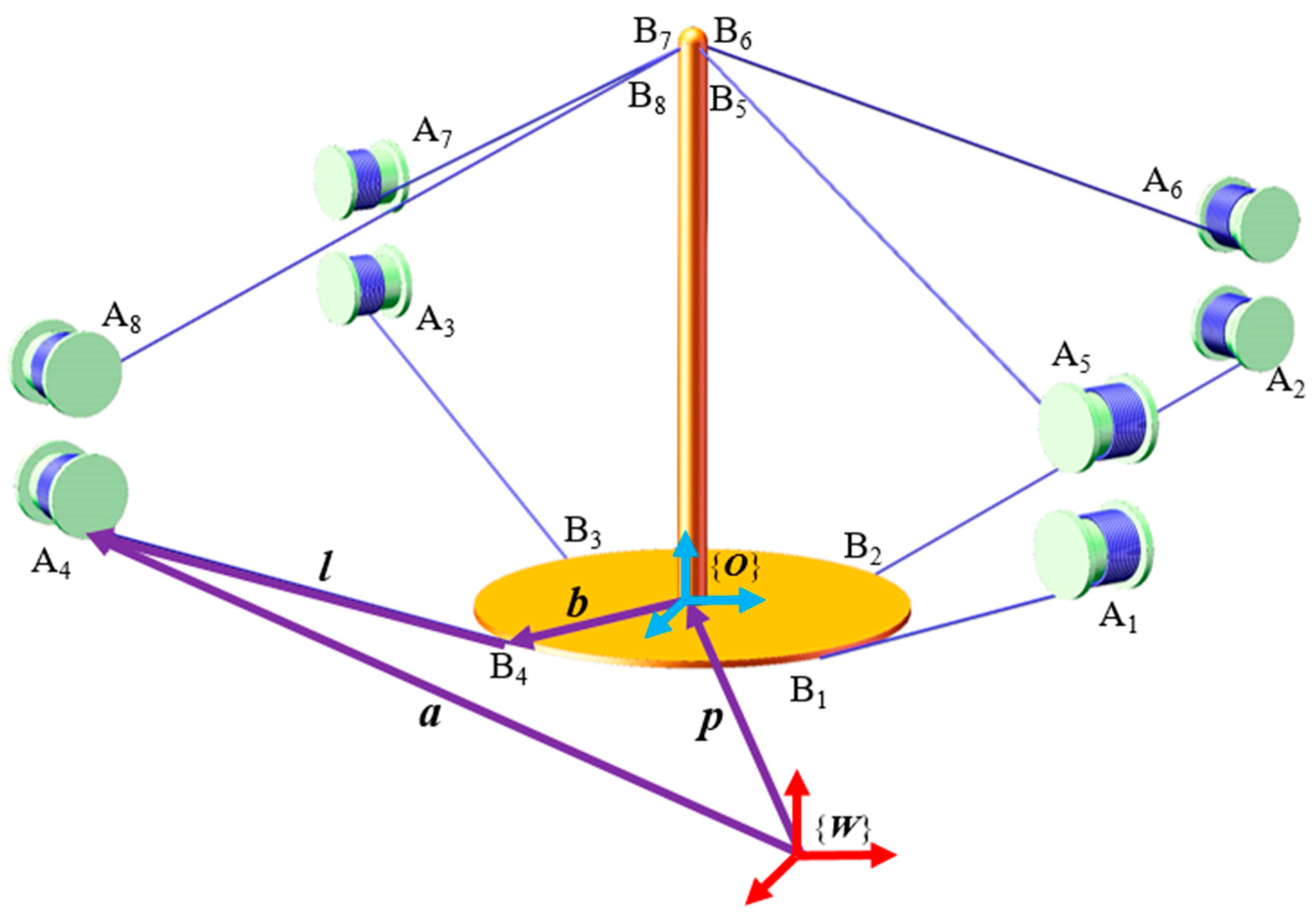
In Figure 2, {W} represents the frame coordinate system, while {O} denotes the coordinate system fixed on the moving platform. The pose of the moving platform is described by the orientation of {O} relative to {W}, represented as [p, θ], where p signifies the position vector and θ denotes the angle vector. The attachment points between the mobile platform and the ropes are labeled as B1, B2, …, B8, while the winding points between the ropes and the winches are denoted as A1, A2, …, A8. In the coordinate system {O}, the coordinates of Bi are denoted as bi, where i ranges from 1 to 8. Similarly, in the coordinate system {W}, the coordinates of Ai are represented as ai, where i ranges from 1 to 8. The length of each rope is represented by the vector li, where i ranges from 1 to 8. The vector geometric relationship between the mobile platform and the rack is described as follows:
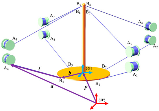
Figure 2.
Schematic diagram of the redundantly constrained cable-driven parallel robot studied in this paper.
Within this context, R is constructed from the rotation matrix calculated from θ. Determining ai given [p, θ] represents the inverse kinematics problem of the mechanism, whereas obtaining [p, θ] given ai constitutes the forward kinematics problem of the mechanism.
In the context of the text, the rope is conceptualized as a parallel spring-damping system capable of exerting unidirectional tension. Here, the deformation coefficient is denoted as k, and the elongation amount and rate of change of each rope are, respectively, represented as ei, where i ranges from 1 to 8. The magnitude of the rope tension is defined as follows:
Here, c denotes the internal damping within the rope. When the elongation amount is less than 0, the tensile force is 0. The elongation of the rope can be computed based on the length of the driving rope and the position of the moving platform:
Here, di represents the length of the driving rope, ||li|| denotes the rope length of the current pose calculated from Equation (1), ||l0i|| represents the rope length of the initial pose, and f0i, where i ranges from 1 to 8, signifies the pre-tension of the rope in the initial pose.
The dynamic model of the mobile platform can be formulated using the Newton–Euler equation:
Here, Io denotes the inertial tensor of the mobile platform; Fw represents the combined force of the rope tension and external load in the coordinate system {W}, and M signifies the mass of the mobile platform. Additionally, To denotes the tension of the rope and the torque of the external load on the center of mass of the mobile platform in the coordinate system {O}, and and denote the angular velocity vector and angular acceleration vector of the mobile platform in the coordinate system {O}. The angular acceleration of the mobile platform in the coordinate system {W} is denoted as , and its relationship with is as follows.
The dynamic model of the mechanism encompasses both a rope dynamic model and a mobile platform dynamic model. The model neglects the mass, lateral vibration, and mutual interference of the rope. In this context, the length of the driving rope serves as the system input, with no consideration of the dynamics of the winch. The simulation results indicate that selecting the length of the driving rope instead of the motor torque is more conducive to the convergence of the training process for the reinforcement learning agent.
3. Methods
3.1. Environment Settings
In reinforcement learning, the environment encompasses the entities with which the agent interacts. It receives actions from the intelligent agent, produces corresponding dynamic responses, and provides feedback to the agent in the form of observation values. Additionally, the environment generates a reward signal to assess the quality of the agent’s actions. Through repeated interactions, the agent learns to make appropriate decisions based on the observed values, refining its behavior-generation strategy to maximize the long-term cumulative rewards [27]. The environment in this context comprises the dynamic model of the system and the interface for interaction with the intelligent agent. These interfaces are responsible for receiving the agent’s actions, providing feedback on observations, rewards, and signals for interaction termination.
In this study, the control objective is to generate a suitable sequence of driving rope lengths, ensuring that the motion posture of the mobile platform is evenly distributed within the given space and that the rope tension remains within specified limits during motion. Based on this control task, it is evident that the actions generated by the agent correspond to the driving rope lengths. The action values can be discrete or continuous. However, for a mechanism with 8 ropes, discretizing the action space of the 8-dimensional vector leads to numerous combinations, necessitating significant computational effort in selecting the optimal action for the agent. Therefore, in practical operation, actions of continuous variable types are preferred to avoid the combinatorial explosion.
The reward function governs the spatial distribution of the mobile platform’s motion posture driven by the intelligent agent. In the article, the design concept of the reward function is articulated as follows: with the target position as the reference, the closer the mobile platform approaches the target position, the higher the reward bestowed upon the agent. Consequently, the agent endeavors to propel the trajectory of the mobile platform as closely as possible along the line connecting the initial position and the target position. Moreover, when confronted with multiple target positions, the trajectory of the mobile platform is steered to distribute near a uniformly planned straight line in space.
Furthermore, the environment encourages the rope tension of the mobile platforms to converge toward the specified value within the predetermined range during motion, mitigating tendencies of tension fluctuations toward the boundary of the range. Should the rope tension surpass the designated range, the environment levies a penalty on the intelligent agent. The expression of the reward function is delineated as follows:
where re represents the reward function value, and k1, k2, k3, k4, k5 are the coefficients of the reward function. Pos denotes the end-effector pose, Postarget represents the target pose, (x, y, z) are the end-effector position coordinates, (xtarget, ytarget, ztarget) are the target position coordinates, δ is a small numerical value, F denotes the cable tension, and Ftarget represents the target tension.
The observations acquired by the intelligent agent from the environment should encompass adequate information to facilitate the adoption of an optimal strategy. While greater informational sufficiency in terms of the observation values renders it easier for the intelligent agent to make optimal judgments, it concurrently complicates the actual measurement process. In this article, the posture of the mobile platform and the tension of the rope serve as observation values, obtainable through cameras and tension sensors. However, a single-step observation value is insufficient to fully map the institutional configuration A. Consequently, the agent cannot perform optimal actions based solely on single-step observations. Nevertheless, through multiple rounds of interaction, the agent can implicitly accumulate adequate information to make optimal decisions. Rewrite the differential Equation (4) as Ft, pt, θt, A. The algebraic form of the implicit functions for these variables:
Similarly, rewrite Equations (2) and (3) as implicit functions as follows:
In the above formula, t represents the current time step, and t+1 represents the next time step, where Ft, pt and θt, respectively, denote the cable tension, end-effector position, and end-effector orientation at the current time step. Ft+1, pt+1, and θt+1, respectively, represent the cable tension, end-effector position, and end-effector orientation at the next time step.
Each observation can be complemented by 6 valid equations derived from Equation (7). The transition from the current observation to the subsequent one can be governed by Equation (8), offering 8 valid equations. Ideally, through interacting with the environment for more than two rounds, the intelligent agent can amass sufficient information to refine its strategy.
In accordance with the control task requirements, a constraint mandates that the rope tension remains within the specified range. Furthermore, a potential constraint dictates that the posture of the mobile platform should also fall within the designated range. Correspondingly, the termination condition of the environment is set to the detection of the rope tension or posture surpassing the specified range.
3.2. Deep Deterministic Policy Gradient
To address the control problem with a continuous action space, the Deep Deterministic Policy Gradient (DDPG) algorithm presents itself as a suitable choice [28,29]. The DDPG adopts an actor–critic architecture, comprising two actor networks (actor network and target actor network) and two critic networks (critic network and target critic network). The actor network models the behavioral strategies of intelligent agents, denoted as μ, parameterized by θμ:
where at represents the action values output by the actor network, and st denotes the current state. The selection of a behavior based on the current state in the fitting of a critic network, denoted as qt, is determined by θQ:
The target actor network, denoted as μ’, and the target critic network, denoted as Q’, share identical structures with their respective actor and critic counterparts. They are parameterized by θμ′ and θQ′ to mitigate the training variance. Throughout the training process, the agent performs actions based on the deterministic policy network, denoted as μ(s). The DDPG introduces random noise to this behavior to enhance the agent’s exploration ability:
Execute action at to obtain reward rt and next state st+1, and store (st, at, rt, st+1) in the experience replay buffer for subsequent updates of the critic and actor. The quality of strategy μ(s), denoted as J, can be evaluated by the expected value of the initial state:
where denotes the expectation of the rewards obtainable by taking action according to the current policy μ(s) given the state s, and is the probability density function of the state. Substituting Equations (9) and (10) into Equation (12) results in:
According to the chain rule of differentiation, taking the gradient of Equation (13) allows for the determination of the update direction of the actor network:
where N denotes the size of the mini-batch randomly sampled from the experience replay buffer, containing experiences (st, at, rt, st+1). In Equation (14), Eμ represents the expected cumulative return obtained by intelligent agents following strategies μ. This expected cumulative return indicates the effectiveness of the strategy. Specifically, Equation (14) represents the gradient of the cumulative expected return with respect to the parameters θ. However, due to the difficulty of calculating the probability distribution of μ and Q in this formula, it is also challenging to directly compute their corresponding gradient with respect to θ. In practical applications, the average gradient of μ and Q relative to θ is often used as a substitute for the expected value. Consequently, the right side of Equation (14) is approximately equal to the right side of Equation (15). The updating of the critic network is accomplished by minimizing the loss function L:
Here, represents the value function objective, which is the sum of the current reward value and the discounted long-term reward. The discount factor is denoted as γ, and is expressed as:
where is the discount factor. To mitigate the training variance, the target actor and target critic are updated smoothly at each time step using the actor and critic:
where is the update coefficient. This dictates the appropriate update intensity for and . Another approach to mitigate the training variance is to update and periodically by assigning them the values of θμ and θQ at specified intervals.
The Algorithm 1 of DDPG is as follows.
| Algorithm 1 Deep Deterministic Policy Gradient (DDPG) | |
| 1. | Initialize actor network μ and critic network Q with random weights θμ and θQ |
| 2. | Initialize target networks μ′ and Q′ with weights θμ′ = θμ and θQ′ = θQ |
| 3. | Initialize replay buffer R |
| 4. | for episode = 1 to M do |
| 5. | Initialize a random process N for action exploration |
| 6. | Receive initial state s1 |
| 7. | for t = 1 to T do |
| 8. | Select action |
| 9. | |
| 10. | Execute action and observe reward rt and new state +1, Store transition (, , rt, +1) in R |
| 11. | Sample a random minibatch of N transitions (, , ri, +1) from R |
| 12. | Set |
| 13. | |
| 14. | Update critic by minimizing the loss: |
| 15. | |
| 16. | Update the actor policy using the sampled policy gradient: |
| 17. | |
| 18. | Update the target networks: |
| 19. | |
| 20. | |
| 21. | end for |
| 22. | end for |
| 23. | return actor network μ and critic network Q |
3.3. Training and Driving
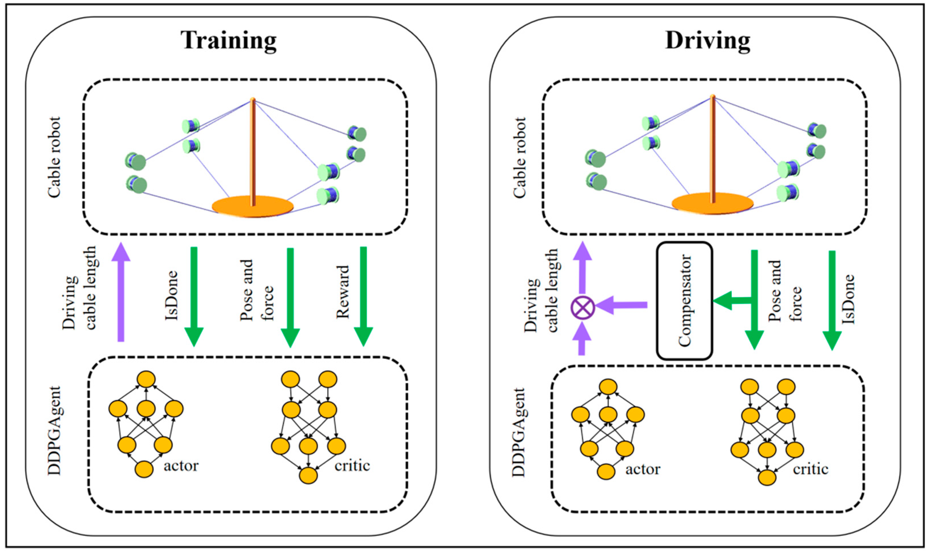
As depicted in Figure 3, throughout the training phase, the agent lacks knowledge of the dynamic model governing the rope mechanism. Through observation of the current pose and rope tension of the moving platform, as well as the subsequent pose and rope tension after executing the prescribed driving rope length, the agent acquires insights into the mechanism’s dynamic model. Leveraging rewards and termination signals, the intelligent agent iteratively refines its behavioral strategy, aiming to maximize the accumulated returns obtained. The ultimate objective of training is to cultivate an intelligent agent capable of effectively driving the cable-driven mechanism to any unknown coordinate Ai. Effective driving entails ensuring that the movement posture of the mobile platform is as evenly distributed as possible within the given space and that the tension of the rope remains within the specified range during the movement process.
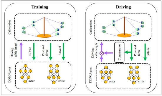
Figure 3.
Training and driving process of reinforcement learning agents for driving the cable-driven robot with unknown parameters.
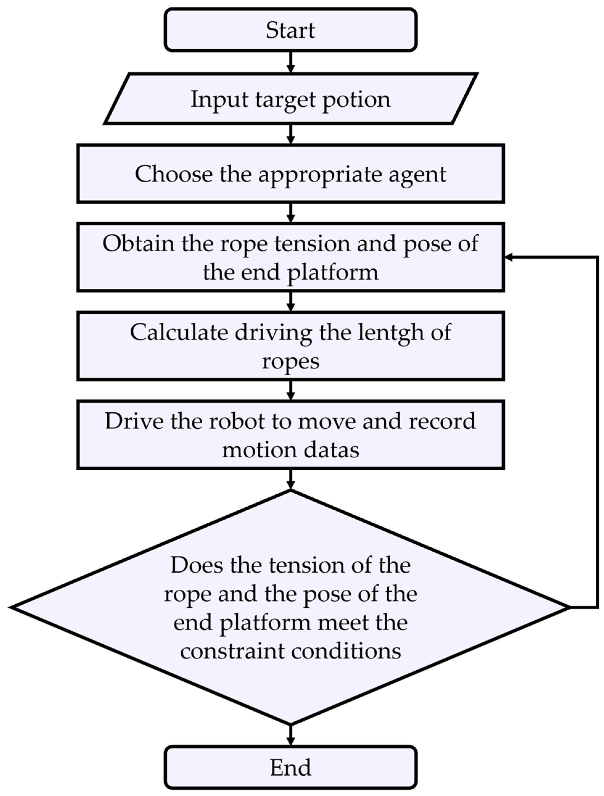
The procedure for employing trained agents to operate a cable-driven parallel robot is as follows Figure 4:
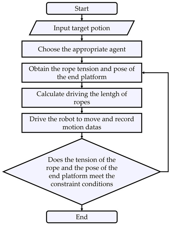
Figure 4.
Flowchart illustrating the process of using trained agents to drive a cable-driven parallel robot.
To alleviate the training complexity and enhance the convergence speed, a practical approach involves maintaining the constant value of Ai while reducing the constraints. The direct notion to enable the intelligent agent to effectively maneuver the mechanism of Ai at any unknown coordinate is to randomly generate Ai in each training round, thereby eliminating the agent’s reliance on a specific Ai value for mechanism control. However, empirical evidence suggests that employing the method of randomly generating Ai can significantly impede the training convergence. Conversely, keeping Ai constant considerably streamlines the training process. Nonetheless, this approach engenders a challenge: the intelligent agent remains effective solely for rope mechanisms within a certain range rather than arbitrary configurations, specifically the neighborhood of Ai that remains unaltered during training. This issue is easily addressed, and we will elucidate how to extend this range to any interval in future studies.
Strict constraints make it easier for agents to terminate training, resulting in the sparsity of effective rewards, which leads to slow learning rates for agents. During actual training, constraints on the upper and lower boundaries of the force and the pose of the moving platform are simplified to solely encompass the maximum load-bearing capacity. In this way, the intelligent agent can more easily manipulate the mobile platform and learn to optimize the tension distribution and attitude space distribution through the reward function. Due to the absence of mandatory lower force boundaries and the mechanism’s nonlinear dynamic characteristics, the strategy network is predisposed to converge toward a local optimal solution. This manifests during the mechanism’s operation by the intelligent agent: certain ropes may slacken, denoted by tension changes to 0. To rectify the rope slackness, a proportional compensator is incorporated during the driving process. When the rope tension falls below the specified value, the compensator outputs a driving rope length proportional to the disparity between the given tension and the detected tension. Conversely, when the rope tension surpasses the specified value, the compensator’s output is set to 0.
Moreover, aside from integrating a compensator into the driving process, another significant disparity between the training and driving processes lies in the differing termination conditions. During the training process, the termination condition is simplified as tension exceeding the given maximum value to reduce the complexity of the training. In the final driving process, comprehensive constraints should be used as termination conditions, including the rope tension exceeding the specified range or the platform posture exceeding the specified range.
4. Results
Table 1 and Table 2 present the dynamic model of the cable-driven mechanism and the parameters utilized during the training process of the intelligent agent, respectively.

Table 1.
Parameters for the dynamic model of the cable-driven mechanism.
Table 2.
Parameters for training agents.
In Table 1, ‘m’ represents the mass of the moving platform, ‘I’ denotes the inertia tensor of the moving platform, ‘k’ signifies the elastic coefficient of the rope, and ‘c’ stands for the damping coefficient. During training, the tangent points of the rope and winch are positioned near the four top corners of the rack. The rack takes the form of a rectangle, with ‘la’, ‘wa’, and ‘ha’ denoting the length, width, and height of the rectangle, respectively. Δh represents the difference between the height of the tangent point between the four upper ropes and the winch and the height of the tangent point between the lower ropes and the winch. ‘lb’ and ‘wb’ represent the length and width of the rectangle where the connection point between the lower rope and the moving platform is situated. ‘db’ refers to the z-coordinate size of the connection point between the lower rope and the moving platform in the moving platform coordinate system, while ‘hb’ denotes the z-coordinate size of the connection point between the upper rope and the moving platform, with its x and y coordinates set to 0. The ‘Ai’ of the institution remains unchanged during training, but the ‘Ai’ of the institution driven by the trained agent is randomly generated. The random generation method entails randomly selecting coordinates in the cube space centered on the ‘Ai’ used during training, with the size of the cube’s edge taken as ‘drnd’. ‘Pos0’ represents the initial pose of the moving platform, while ‘Posb’ specifies the constraint space for the pose of the moving platform, with the boundaries of each dimension in the constraint space given by ‘Pos0i ± Posbi’, where ‘i = 1,2, …,6’. ‘Fmin’ and ‘Fmax’ denote the minimum and maximum values of the tension of the rope to be ensured during the final driving process.
Table 2 displays the parameter values associated with the training agents. ‘Action’ refers to the length of the driving rope output by each agent, ranging from −0.003 m to 0.003 m. ‘Ts’ represents the sampling time of the intelligent agent in the environment, while ‘Tf’ denotes the runtime of the simulation, which also serves as the maximum duration of each episode. The maximum number of time steps per episode is determined by ‘Ts’ and ‘Tf’. The range of the running trajectory of the moving platform is determined by the maximum number of time steps and the range of actions.
The Postarget of the reward function is set to four different coordinates, namely (0.8, 0, 0.75), (0, 0.8, 0.75), (0.4, -0.4, 0.75), and (−0.4, −0.4, 0.75). Four agents are trained with different driving directions for these four different Postarget. The value of Ftarget in the reward function is 20, and the values of k1, k2, k3, k4 and k5 are 100, 20, 20, 20, 20 and 0.1, respectively.
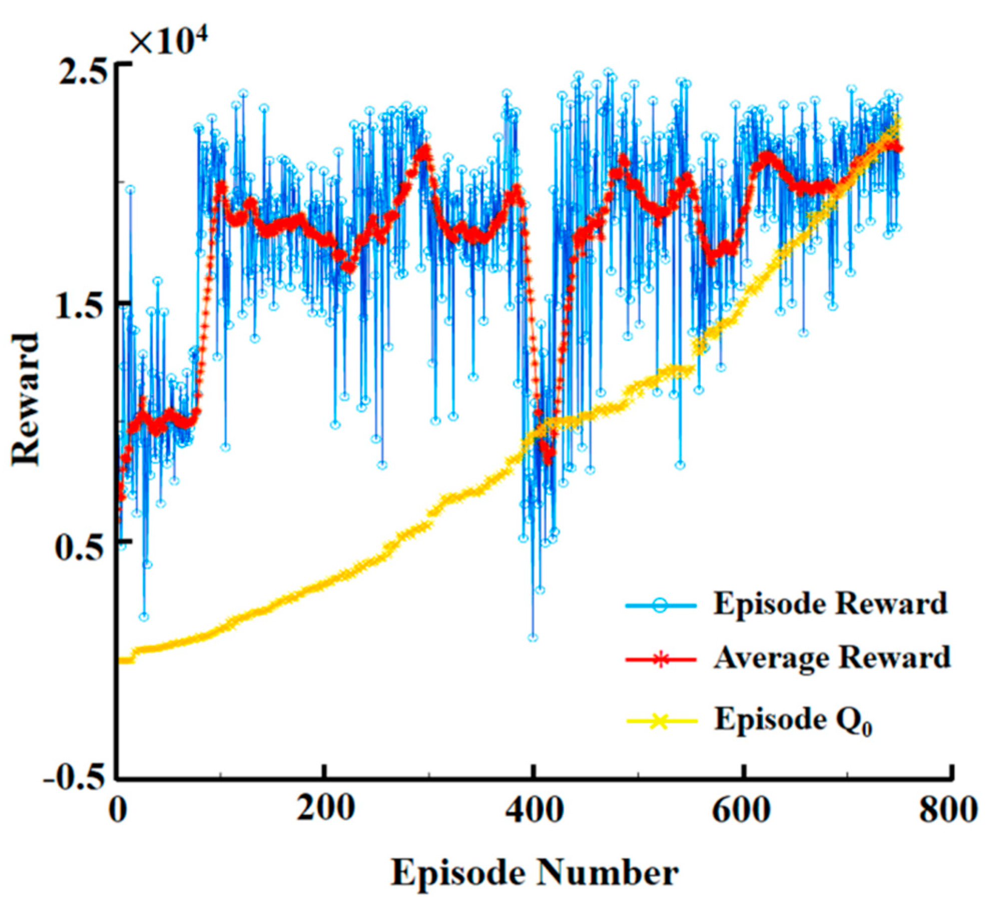
The cumulative rewards obtained by the intelligent agent throughout the training process are illustrated in Figure 5. The training process terminates after 800 episodes. Using a CPU model i7-8700k with six threads running in parallel, the training time is approximately 30 min, demonstrating a satisfactory training speed. In this article, the simulation and testing of the algorithm were carried out using TensorFlow-2.8.0. The DDPG intelligent agent was implemented utilizing the TF-Agents library. Ultimately, the agents were exported to a C# environment to enable motion control of a physical cable-driven parallel robot within the C# framework.

Figure 5.
Training process for the agent. Each episode depicts one driving process of the mechanism using the agent. The cumulative reward obtained during the driving process serves as the reward value for that episode.
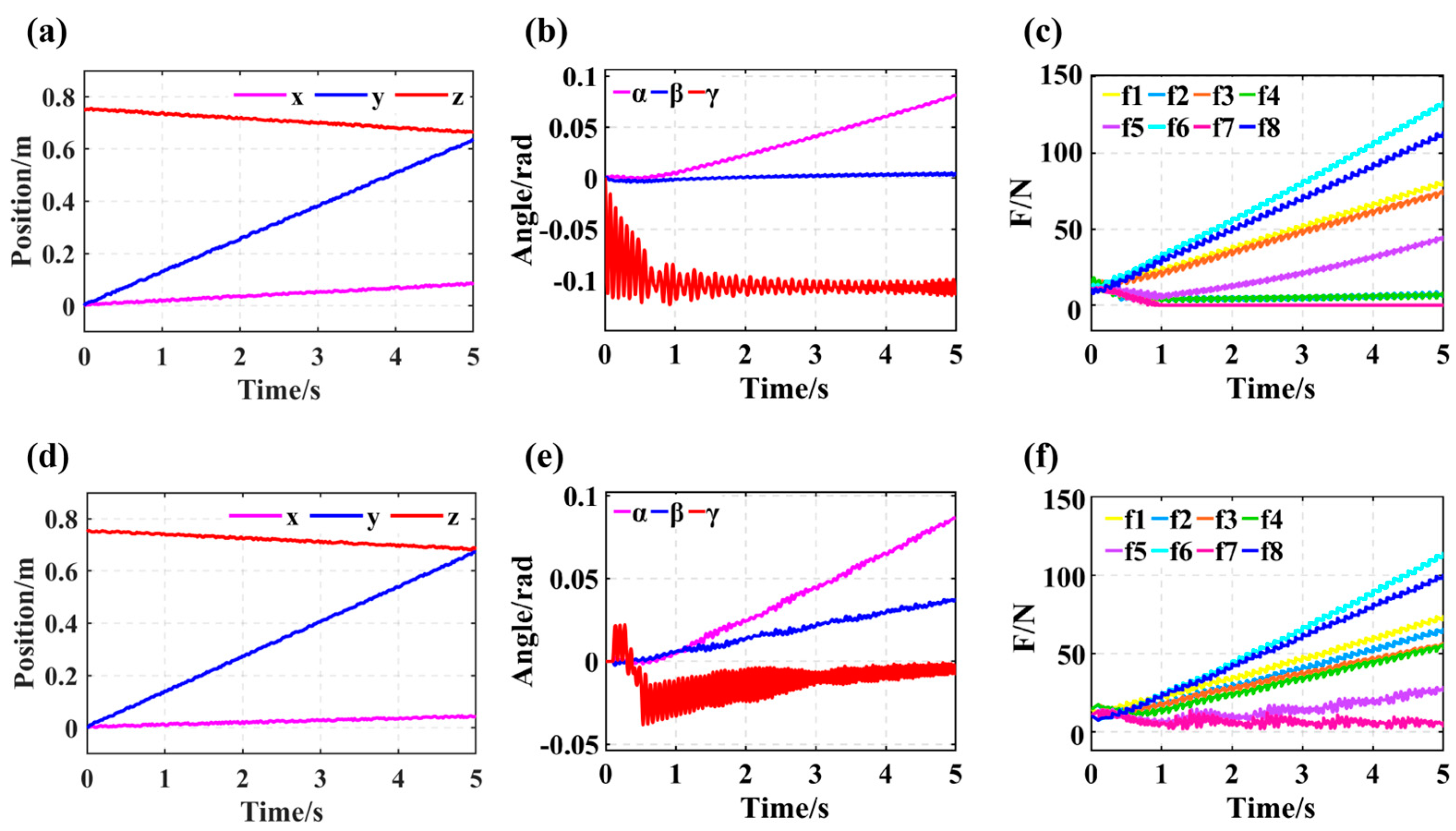
After terminating the training, an agent is employed to conduct driving tests on randomly generated Ai mechanisms to assess the agent’s generalization capability. The target point coordinates for the driving are (0, 0.8, 0.75). Figure 6 depicts the pose and rope tension of the mobile platform during the driving process. Figure 6a–c represent results without the tension compensator driving, while Figure 6d–f depict results with the tension compensator driving added. It is evident that regardless of the presence of a compensator, the agent ensures the movement of the platform toward the target point with minimal turning angles. Upon adding a compensator, the tension, initially below the set minimum value, increases to near the set minimum value, ensuring all the ropes in the drive are tensioned. Furthermore, there are observable changes in the mobile platform’s pose before and after adding the compensator. However, multiple driving tests indicate that the addition of a compensator does not lead to significant changes in the pose, thereby maintaining the pose constraints.
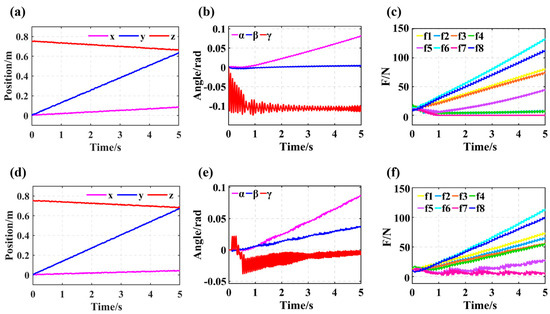
Figure 6.
Simulation results of driving cable-driven robots with unknown parameters using trained agents. (a) Variation in the end-effector position during the driving process. (b) Variation in the end-effector orientation during the driving process. (c) Variation in the cable tensions during the driving process. (d) Variation in the end-effector position during the driving process with the tension compensator. (e) Variation in the end-effector orientation during the driving process with the tension compensator. (f) Variation in the cable tensions during the driving process with the tension compensator.
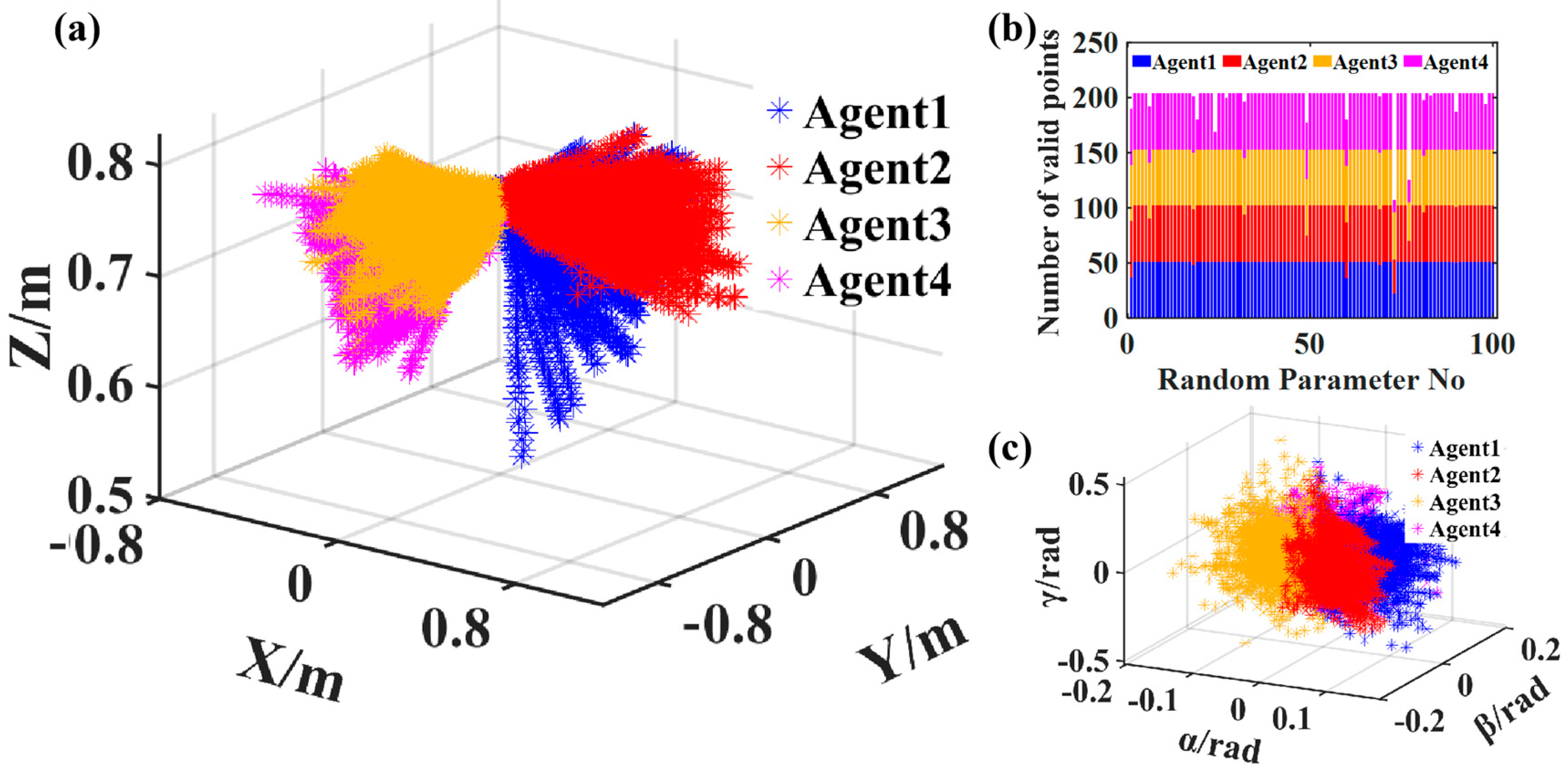
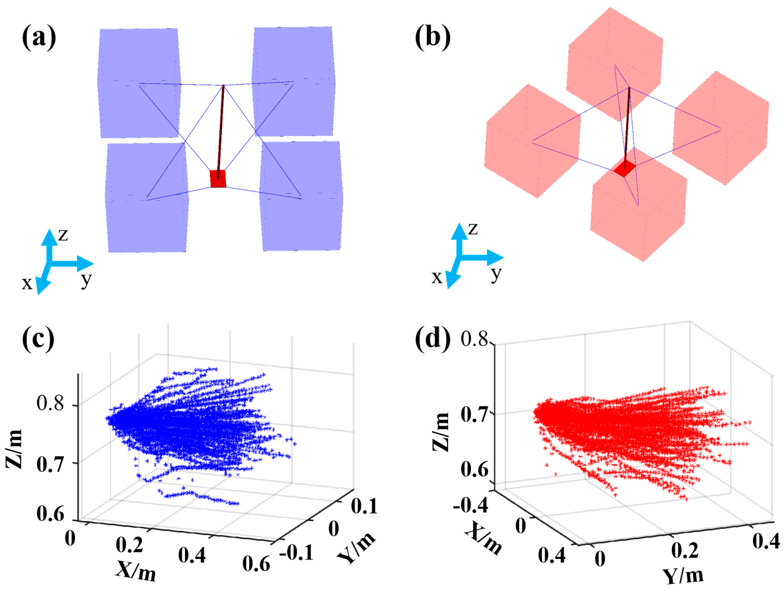
Figure 7 presents the results of multiple drives for several mechanisms with randomly selected parameters. For 100 randomly configured mechanisms, 4 trained intelligent agents were employed for the driving. In Figure 7a, the spatial distribution of the driving trajectories is depicted, illustrating the evident directionality of the driving trajectories generated by each agent for different unknown mechanisms, which facilitates the generation of uniformly distributed trajectories in space. The stronger the directional tendency of the trajectories generated by the agents, the better the assurance of a uniform spatial distribution of the trajectories. This can be achieved by setting relatively uniform target points. Conversely, if an agent’s driving trajectories lack obvious directionality, the trajectories generated by different agents may cluster in a corner of space, rendering the acquired data unable to fully reflect the characteristics of the mechanisms, thereby impeding accurate parameter identification.

Figure 7.
Results of driving a cable-driven robot with 100 unknown parameters using 4 trained agents. (a) Spatial distribution of the mechanism’s trajectory during the driving process. (b) Statistical results of the effective sampling points during the driving process. (c) Variation of the end-effector orientation during the driving process.
Figure 7b illustrates the statistical distribution of 100 driving trajectory points. In the simulation setup, the maximum data sampling limit for a single drive is set to 200. The actual number of valid points obtained depends on when the intelligent agent violates the constraint conditions during the mechanism’s operation. Specifically, if the tension and terminal platform of the mechanism driven by the intelligent agent remain within the specified range throughout the entire motion process, 200 data points can be collected. If the constraint conditions are violated at the beginning of the driving phase, leading to premature termination, only a small amount of data will be collected. In the 100 tests conducted, only 2 trajectory data points were below 150. According to the results, the number of effective data points accounts for 98% of the total planned data points. The results suggest that utilizing trained intelligent agents to operate a rope mechanism with randomly selected parameters can yield ample motion data.
Figure 7c delineates the angular distribution of the mobile platform during testing. It can be observed that α and β fall within the range of −0.2 to 0.2 radians, while γ ranges from −0.5 to 0.5 radians. The minimal angular rotation of the mobile platform during operation does not induce interference among the ropes, thereby affirming the validity of disregarding the assumption of rope interference in the mechanism’s dynamic modeling.
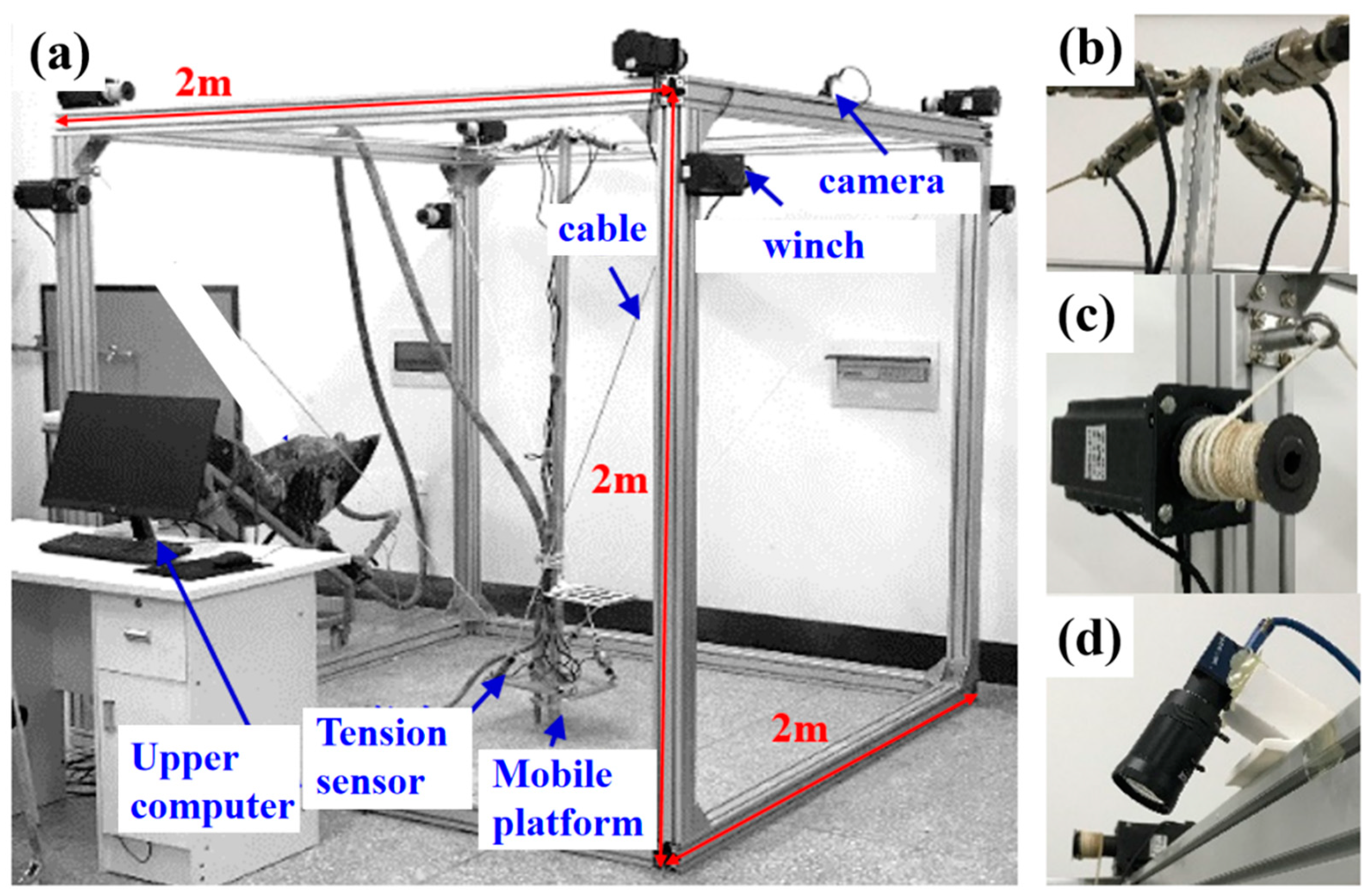
The experimental setup employed in this study comprises an eight-rope six-degree-of-freedom redundant constrained rope driving mechanism, as depicted in Figure 8. The driving elements of this mechanism consist of 86-step motors and rope pulley systems. The end moving platform is constructed with a rectangular plate affixed to a perpendicular rod. The tension sensors are connected in series between the rope and the end moving platform. Data acquisition is facilitated through a data acquisition card, with tension readings from the eight ropes transmitted to the host computer via the RS485 bus. To mitigate the impact of the sensor weight, conduct a zero-tension program at the origin position of the end platform before initiating each operation of the rope mechanism. The end platform’s pose is determined through a monocular vision system, which operates on the principle of acquiring the external parameters of the camera relative to the target. A detailed methodology regarding the construction and operation of the monocular vision system is provided in the Supplementary Materials. The monocular vision system used in this study consists of an industrial camera fixed on the frame and a calibration disk fixed on the end platform. Sampling occurs at a rate of 30 frames per second, enabling accurate and real-time pose estimation.
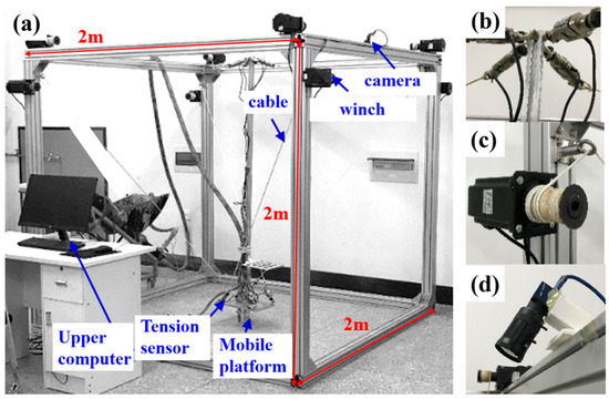
Figure 8.
The cable-driven parallel robot used in the experiment. (a) The cable-driven parallel robot system. (b) The tension sensor used for measuring the cable tensions. (c) The winch of the cable-driven robot. (d) The monocular camera fixed on the frame.
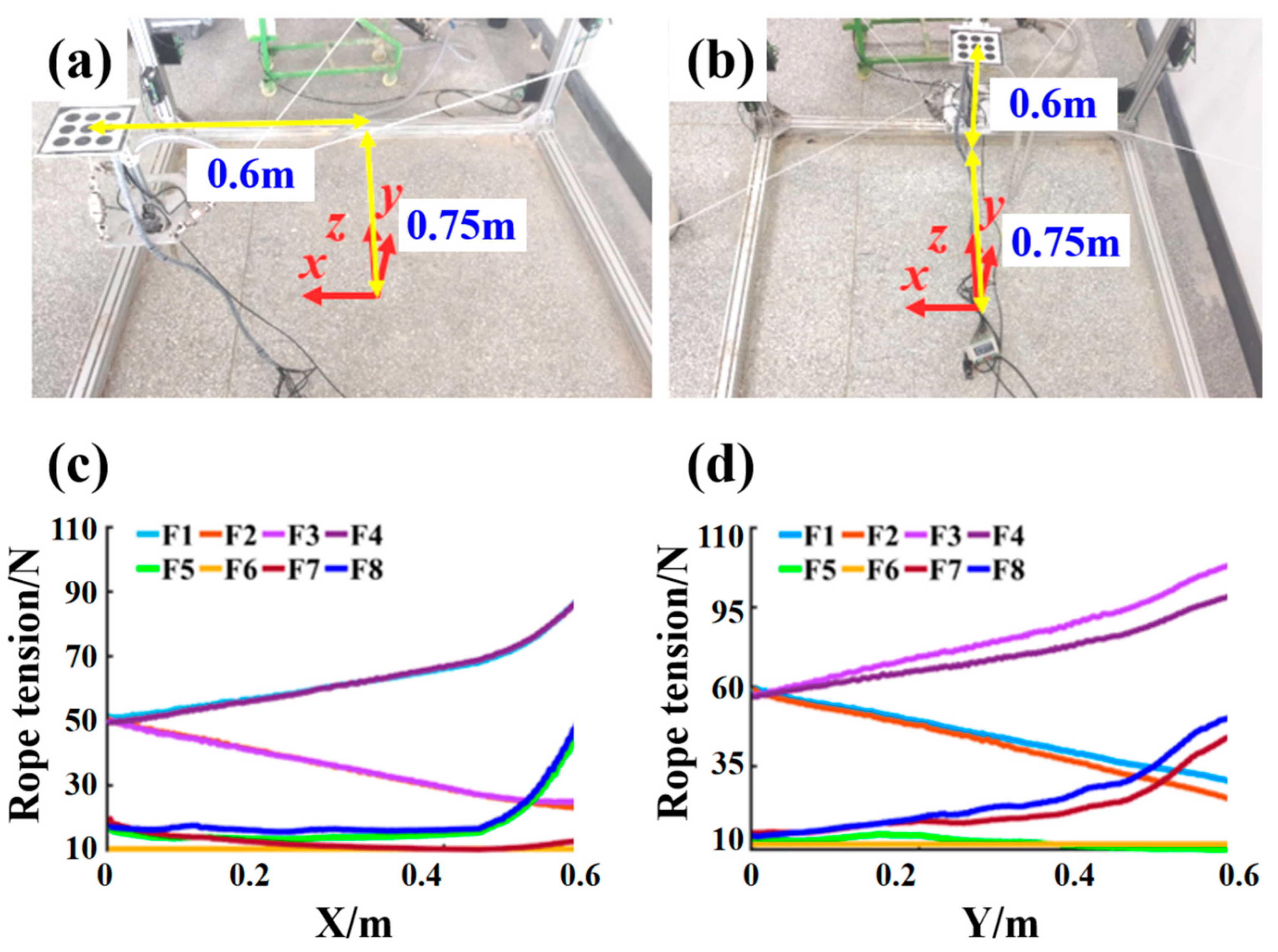
Figure 9 presents the experimental outcomes of driving the trained agent within a physical system. By selecting target points (0.8, 0, 0.75) and (0, 0.8, 0.75) to navigate the rope device, Figure 9a,b exhibit the actual driving results. Evidently, the end platform is successfully propelled toward the vicinity of the target point along a coarse trajectory. Despite the modest motion accuracy of the mechanism, this outcome is deemed satisfactory due to the discernible directional trajectory, which facilitates the acquisition of ample effective sampling data for the subsequent mechanism parameter calibration.
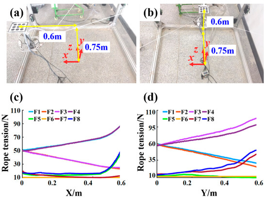
Figure 9.
Results of driving the cable-driven mechanism using trained agents. (a) Results of driving the cable-driven mechanism toward the target point (0.8, 0, 0.75). (b) Results of driving the cable-driven mechanism toward the target point (0, 0.8, 0.75). (c) Variation of the cable tensions during the driving process toward the target point (0.8, 0, 0.75). (d) Variation of the cable tensions during the driving process toward the target point (0, 0.8, 0.75).
Figure 9c,d depict the measured tension values of the rope along the trajectory. Notably, the rope tension remains below 110 N throughout the entire movement process, falling below the prescribed threshold of 150 N. Thanks to the tension compensator introduced in Section 3, the minimum tension of each rope remains around 10 N, effectively preventing rope relaxation. The initial tension of the rope is established by the pre-tension force applied to the end platform at the origin. From Figure 9c,d, it can be observed that the initial tension and pre-tension of the two driving processes are not identical, indicating the robustness of the trained intelligent agent against minor variations in the pre-tension within the mechanism.
The experimental results indicate that employing reinforcement learning to drive CDPRs with unknown parameters effectively facilitates the collection of motion data essential for subsequent parameter identification.
5. Discussion
The simulations and experiments conducted above have configured parameters Ai within specified ranges. When the range of Ai values expands, the efficacy of the obtained agent’s driving capabilities diminishes, potentially rendering it ineffective. This article presents an extension of the method used to accommodate mechanisms with arbitrarily configured parameters Ai in space. Figure 10a illustrates the configuration of the mechanism in both the simulation and experiment settings mentioned previously. The light blue cube symbolizes the random value space of Ai in the driving tests. In Figure 10c, the trajectory during the driving test of agent1 trained with target position values (0.8, 0, 0.75) is depicted. The mechanism configuration in Figure 10b is obtained by rotating the configuration shown in Figure 10a around the z-axis by −45°. Similarly, the target pose is obtained by rotating the target pose by 45° around the z-axis. Agent1′ is then trained using the mechanism configuration shown in Figure 10b. Subsequently, agent1′ is employed to drive the mechanism with randomly selected values of Ai within the red cube, resulting in the trajectory distribution depicted in Figure 10d.

Figure 10.
Results of driving the mechanism with rotated parameters using reinforcement learning. (a) Range of parameter values before rotation. The blue area represents the spatial range of the randomly selected mechanism coordinates. (b) Range of parameter values after rotation. The red area represents the spatial range of the randomly selected mechanism coordinates. (c) Randomly select 100 sets of parameters from the blue area in (a), and employ reinforcement learning to drive the mechanisms corresponding to these parameters, resulting in a trajectory distribution. (d) Randomly select 100 sets of parameters from the red area in (b), and employ reinforcement learning to drive the mechanisms corresponding to these parameters, resulting in a trajectory distribution.
A comparison between Figure 10c,d reveals a strikingly similar trajectory distribution, albeit with spatial rotation. This aligns with the intuitive expectation that irrespective of transformations in the mechanism’s coordinate system relative to the world coordinate system, as long as the intelligent agent can perceive changes in the pose and rope tension of the end platform relative to the mechanism’s coordinate system, effective driving is achievable. However, the driving trajectory undergoes similar transformations to the mechanism’s coordinate system. Though agent1 may struggle to drive the mechanism configured by Ai in the red cube space, it can still be driven through subsequent transformations. For instance, for the mechanism depicted in Figure 10b, rotating the end platform pose coordinates around the z-axis by 45° and transferring these rotated coordinates and the rope tension to the intelligent agent trained in Figure 10a can yield an effective driving trajectory. Finally, rotating the driving trajectory around the z-axis by −45° produces the trajectory of the mechanism driven by the agent in Figure 10b. It is essential to note that while the transformation of the mechanism in Figure 10b relative to Figure 10a is understood, in reality, the coordinate relationship between the mechanism and Figure 10a remains unknown. This challenge can be addressed by employing a finite number of transformations to rotate Figure 10a and cover the entire space. Simulation experiments demonstrate that for a 2 m × 2 m × 2 m rack mechanism, each agent can effectively drive the mechanism with Ai values within a 1 m × 1 m × 1 m configuration cube. This indicates that only a limited number of transformations are required to fully encompass the configuration space of interest. Various transformations can be attempted to practically drive the mechanism. Given that these transformations span the entire space, effective driving operations corresponding to each transformation can be identified to drive and sample any mechanism with unknown parameters.
An alternative approach to extending the proposed method to mechanisms with arbitrary parameters involves discretizing the space into effective red cube subspaces, as illustrated in Figure 10b. A set of intelligent agents can then be trained for each scenario using the method described in this article. Subsequently, different intelligent agents can be tested to drive the mechanism in practice.
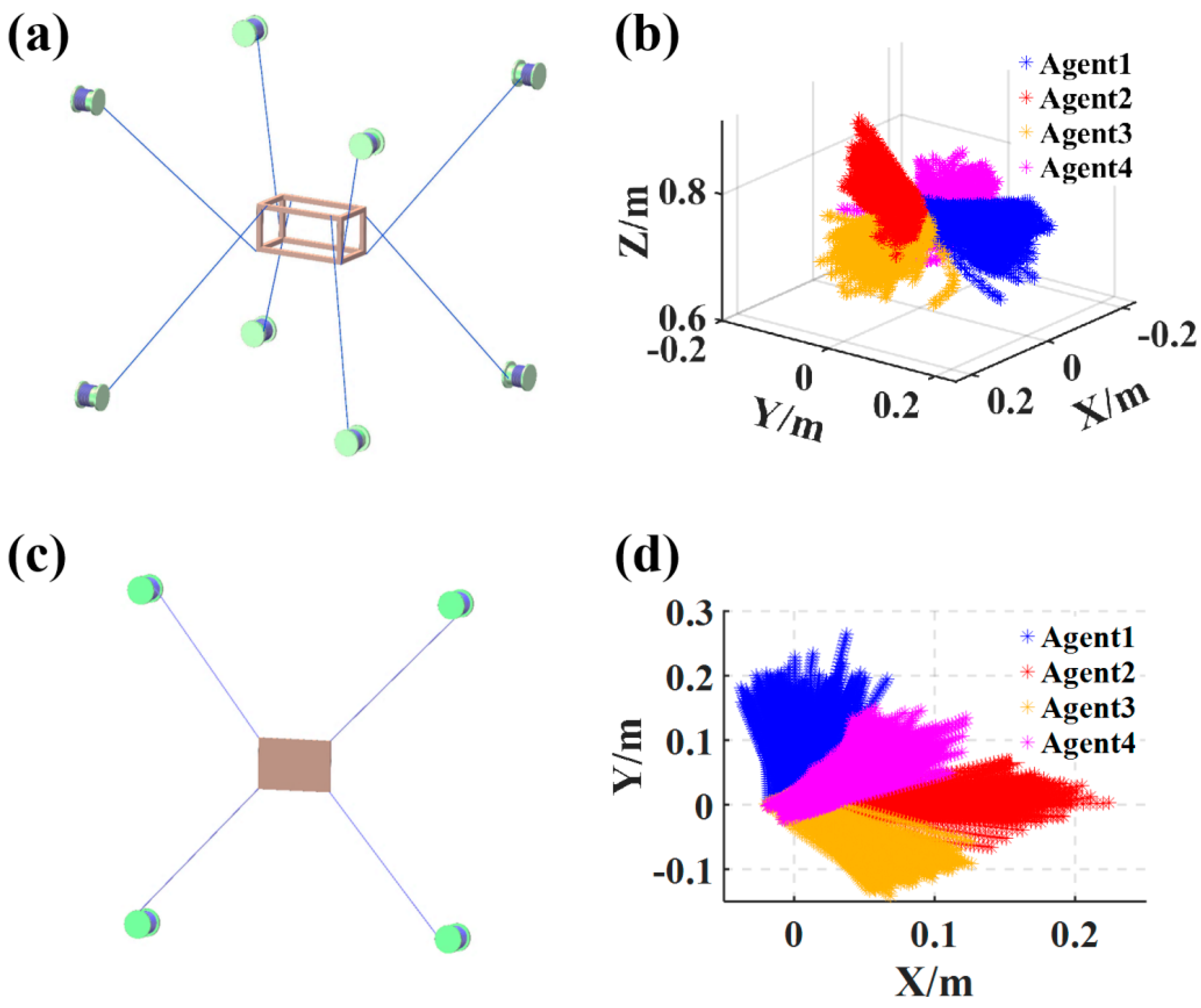
To verify the universality of the method for redundantly constrained cable-driven mechanisms, simulations were conducted on the spatial eight-rope mechanism and the planar four-rope mechanism illustrated in Figure 11. As can be seen from Figure 11b,d, the driving trajectory exhibits clear directionality and both generate sufficient effective motion data. This confirms the method’s applicability to other redundantly constrained cable-driven mechanisms.
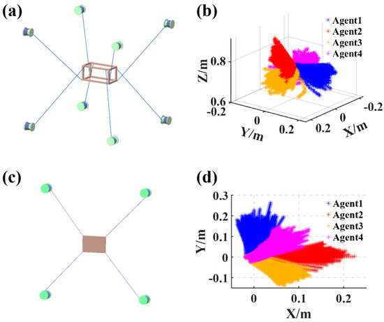
Figure 11.
Results of driving different cable-driven mechanisms using reinforcement learning. (a) Another type of 8-cable, 6-DOF cable-driven parallel robot. (b) Trajectory distribution of the robot in (a) driven by reinforcement learning. (c) Planar 4-cable, 3-DOF cable-driven parallel robot. (d) Trajectory distribution of the robot in (c) driven by reinforcement learning.
In fact, attempts were made to apply the method to under-constrained cable-driven parallel robots; however, the results indicated challenges in addressing the rope relaxation issues during driving through simple compensatory measures. This forms part of our future research plans, aiming to leverage reinforcement learning for effectively driving under-constrained cable-driven parallel robots with unknown parameters.
6. Conclusions
This paper proposes employing reinforcement learning to drive redundant constrained cable-driven robots with unknown parameters. A dynamic model of the cable-driven robot is established, and this model is utilized to construct an environment for interaction with the reinforcement learning agent. A method is adopted during training to reduce the constraints and increase the proportional compensators during driving, thereby reducing the training difficulty and improving the convergence speed. Using the trained reinforcement learning agent, the cable-driven mechanisms corresponding to 100 randomly generated parameter sets are driven, resulting in the simulated trajectories demonstrating a distinct directional spatial distribution. The driving results show that the rope tension corresponding to 98% of the trajectory points is within the specified tension range. Driving experiments conducted on a physical cable-driven setup demonstrate that the rope tension remains within the specified range throughout the driving process, successfully maneuvering the end platform near the designated target point. The simulation and experimental results indicate that this method effectively drives redundant constrained cable-driven robots with unknown parameters to produce directed trajectory distributions and ample sampled data, validating the proposed approach. The application of this method extends from mechanisms with parameters randomly selected within a given region to those with parameters arbitrarily selected, and from specialized configurations of cable-driven robots to various configurations of redundant constrained cable-driven robots. Thus, reinforcement learning emerges as a powerful tool for facilitating the rapid reconstruction of cable-driven robots. In future research, to enable the operation of under-constrained cable-driven parallel robots with unknown parameters, we will employ reinforcement learning agents to interact with the robot and predict its tension distribution space. Subsequently, we will plan a path within this tension distribution space to achieve effective control of the under-constrained cable-driven parallel robot with unknown parameters.
Supplementary Materials
The following supporting information can be downloaded at: https://www.mdpi.com/article/10.3390/machines12060372/s1, Figure S1: Critic neural network structure and actor neural network structure of DDPG; Figure S2: Schematic diagram of Monocular Stereo Vision P3P problem; Figure S3: A monocular stereo vision system constructed using an industrial camera and a target; Table S1: Parameters for neural network.
Author Contributions
Conceptualization, D.Z.; Methodology, D.Z.; Software, D.Z.; Validation, D.Z.; Formal analysis, D.Z.; Data curation, D.Z.; Writing—original draft, D.Z.; Visualization, D.Z.; Supervision, B.G.; Project administration, B.G. All authors have read and agreed to the published version of the manuscript.
Funding
This research received no external funding.
Data Availability Statement
Data are contained within the article.
Acknowledgments
I extend my gratitude to Guo Bin for his invaluable guidance during the problem exploration and experimental implementation.
Conflicts of Interest
The authors declare no conflict of interest.
References
- Liu, F.; Song, Z.; Ma, J. Modeling and analysis of a cable-driven serial-parallel manipulator. Proc. Inst. Mech. Eng. Part C J. Mech. Eng. Sci. 2024, 238, 1012–1028. [Google Scholar] [CrossRef]
- Zarebidoki, M.; Dhupia, J.S.; Xu, W. A review of cable-driven parallel robots: Typical configurations, analysis techniques, and control methods. IEEE Robot. Autom. Mag. 2022, 29, 89–106. [Google Scholar] [CrossRef]
- Qian, S.; Jiang, X.; Qian, P.; Zi, B.; Zhu, W. Calibration of Static Errors and Compensation of Dynamic Errors for Cable-driven Parallel 3D Printer. J. Intell. Robot. Syst. 2024, 110, 31. [Google Scholar] [CrossRef]
- Chesser, P.C.; Wang, P.L.; Vaughan, J.E.; Lind, R.F.; Post, B.K. Kinematics of a cable-driven robotic platform for large-scale additive manufacturing. J. Mech. Robot. 2022, 14, 021010. [Google Scholar] [CrossRef]
- Williams, R.L.; Graf, E. Eight-cable robocrane extension for NASA JSC argos. In Proceedings of the International Design Engineering Technical Conferences and Computers and Information in Engineering Conference, Virtual, Online, 17–19 August 2020. [Google Scholar]
- Li, H.; Sun, J.; Pan, G.; Yang, Q. Preliminary running and performance test of the huge cable robot of FAST telescope. In Proceedings of the Cable-Driven Parallel Robots: Proceedings of the Third International Conference on Cable-Driven Parallel Robots, Quebec, QC, Canada, 2–4 August 2017; pp. 402–414. [Google Scholar]
- Kuan, J.Y.; Pasch, K.A.; Herr, H.M. A high-performance cable-drive module for the development of wearable devices. IEEE/ASME Trans. Mechatron. 2018, 23, 1238–1248. [Google Scholar] [CrossRef]
- Zheng, Y.; Zhao, S. Calculation principle of dynamic derivatives for wire-driven parallel suspension systems used in forced oscillation experiments in low-speed wind tunnels. In Proceedings of the International Conference on Automatic Control and Artificial Intelligence (ACAI 2012), Xiamen, China, 3–5 March 2012; pp. 622–626. [Google Scholar]
- Sun, Y.; Liu, Y.; Lueth, T.C. Optimization of stress distribution in tendon-driven continuum robots using fish-tail-inspired method. IEEE Robot. Autom. Lett. 2022, 7, 3380–3387. [Google Scholar] [CrossRef]
- Chen, X.; Yao, J.; Li, T.; Li, H.; Zhou, P.; Xu, Y.; Zhao, Y. Development of a multi-cable-driven continuum robot controlled by parallel platforms. J. Mech. Robot. 2021, 13, 021007. [Google Scholar] [CrossRef]
- Lau, D. Initial length and pose calibration for cable-driven parallel robots with relative length feedback. In Proceedings of the Cable-Driven Parallel Robots: Proceedings of the Third International Conference on Cable-Driven Parallel Robots, Quebec, QC, Canada, 2–4 August 2017; pp. 140–151. [Google Scholar]
- Yuan, H.; You, X.; Zhang, Y.; Zhang, W.; Xu, W. A novel calibration algorithm for cable-driven parallel robots with application to rehabilitation. Appl. Sci. 2019, 9, 2182. [Google Scholar] [CrossRef]
- He, Z.; Lian, B.; Song, Y.; Sun, T. Kinematic Parameter Identification for Parallel Robots With Passive Limbs. IEEE Robot. Autom. Lett. 2023, 9, 271–278. [Google Scholar] [CrossRef]
- Luo, X.; Xie, F.; Liu, X.-J.; Xie, Z. Kinematic calibration of a 5-axis parallel machining robot based on dimensionless error mapping matrix. Robot. Comput.-Integr. Manuf. 2021, 70, 102115. [Google Scholar] [CrossRef]
- Gouttefarde, M.; Lamaury, J.; Reichert, C.; Bruckmann, T. A versatile tension distribution algorithm for $ n $-DOF parallel robots driven by n + 2 cables. IEEE Trans. Robot. 2015, 31, 1444–1457. [Google Scholar] [CrossRef]
- Geng, X.; Li, M.; Liu, Y.; Li, Y.; Zheng, W.; Li, Z. Analytical tension-distribution computation for cable-driven parallel robots using hypersphere mapping algorithm. Mech. Mach. Theory 2020, 145, 103692. [Google Scholar] [CrossRef]
- Lim, W.B.; Yeo, S.H.; Yang, G. Optimization of tension distribution for cable-driven manipulators using tension-level index. IEEE/ASME Trans. Mechatron. 2013, 19, 676–683. [Google Scholar] [CrossRef]
- Song, D.; Zhang, L.; Xue, F. Configuration optimization and a tension distribution algorithm for cable-driven parallel robots. IEEE Access 2018, 6, 33928–33940. [Google Scholar] [CrossRef]
- Xiong, H.; Diao, X. Cable tension control of cable-driven parallel manipulators with position-controlling actuators. In Proceedings of the 2017 IEEE International Conference on Robotics and Biomimetics (ROBIO), Macau, Macao, 5–8 December 2017; pp. 1763–1768. [Google Scholar]
- Sharifani, K.; Amini, M. Machine learning and deep learning: A review of methods and applications. World Inf. Technol. Eng. J. 2023, 10, 3897–3904. [Google Scholar]
- Xiong, H.; Zhang, L.; Diao, X. A learning-based control framework for cable-driven parallel robots with unknown Jacobians. Proc. Inst. Mech. Eng. Part I J. Syst. Control Eng. 2020, 234, 1024–1036. [Google Scholar] [CrossRef]
- Piao, J.; Kim, E.-S.; Choi, H.; Moon, C.-B.; Choi, E.; Park, J.-O.; Kim, C.-S. Indirect force control of a cable-driven parallel robot: Tension estimation using artificial neural network trained by force sensor measurements. Sensors 2019, 19, 2520. [Google Scholar] [CrossRef] [PubMed]
- Nomanfar, P.; Notash, L. Reinforcement Learning Control for Cable-Driven Parallel Robot. 2023. Available online: https://www.researchgate.net/publication/380359761_Reinforcement_Learning_Control_for_Cable-Driven_Parallel_Robot_Comprehensive_Exam_Report (accessed on 8 May 2024).
- Xiong, H.; Xu, Y.; Zeng, W.; Zou, Y.; Lou, Y. Data-Driven Kinematic Modeling and Control of a Cable-Driven Parallel Mechanism Allowing Cables to Wrap on Rigid Bodies. IEEE Trans. Autom. Sci. Eng. 2023. [Google Scholar] [CrossRef]
- Xu, G.; Zhu, H.; Xiong, H.; Lou, Y. Data-driven dynamics modeling and control strategy for a planar n-DOF cable-driven parallel robot driven by n+ 1 cables allowing collisions. J. Mech. Robot. 2024, 16, 051008. [Google Scholar] [CrossRef]
- Zhang, Z.; Yang, L.; Sun, C.; Shang, W.; Pan, J. CafkNet: GNN-Empowered Forward Kinematic Modeling for Cable-Driven Parallel Robots. arXiv 2024, arXiv:2402.18420. [Google Scholar]
- Ernst, D.; Louette, A. Introduction to Reinforcement Learning. 2024. Available online: http://blogs.ulg.ac.be/damien-ernst/wp-content/uploads/sites/9/2024/02/Introduction_to_reinforcement_learning.pdf (accessed on 8 May 2024).
- Tiong, T.; Saad, I.; Teo, K.T.K.; bin Lago, H. Deep reinforcement learning with robust deep deterministic policy gradient. In Proceedings of the 2020 2nd International Conference on Electrical, Control and Instrumentation Engineering (ICECIE), Kuala Lumpur, Malaysia, 28 November 2020; pp. 1–5. [Google Scholar]
- Afzali, S.R.; Shoaran, M.; Karimian, G. A Modified Convergence DDPG Algorithm for Robotic Manipulation. Neural Process. Lett. 2023, 55, 11637–11652. [Google Scholar] [CrossRef]
Disclaimer/Publisher’s Note: The statements, opinions and data contained in all publications are solely those of the individual author(s) and contributor(s) and not of MDPI and/or the editor(s). MDPI and/or the editor(s) disclaim responsibility for any injury to people or property resulting from any ideas, methods, instructions or products referred to in the content. |
© 2024 by the authors. Licensee MDPI, Basel, Switzerland. This article is an open access article distributed under the terms and conditions of the Creative Commons Attribution (CC BY) license (https://creativecommons.org/licenses/by/4.0/).