Abstract
The lack of real-world data on Connected and Autonomous Vehicles (CAVs) has prompted researchers to rely on simulations to assess their societal impacts. However, few studies address the operational and technological challenges of integrating CAVs into existing transport systems. This paper introduces a new CAV driving model featuring a constant time gap longitudinal control algorithm that accounts for sensor errors and platoon formations of varying sizes. Additionally, it develops a high-level route-based decision-making algorithm for CAV path choice. These algorithms were tested in a calibrated motorway corridor simulation, examining different market penetration rates, platoon sizes, and sensor error scenarios. Traffic conflicts were used as a primary safety performance indicator. The findings indicate that CAV sensors are generally adequate, but optimal platoon sizes vary with market penetration rates. To further explore factors influencing traffic conflicts, a hierarchical Bayesian negative binomial regression model was used. This model revealed that in addition to unobserved heterogeneity and spatial autocorrelation, the standard deviation of speeds between lanes and the CAV market penetration rate significantly affect conflict occurrences. These results corroborate the simulation outcomes, enhancing our understanding of CAV deployment impacts on traffic safety.
1. Introduction
Connected and Autonomous Vehicle (CAV) technology has advanced significantly over the past few years. As the deployment of CAVs in the road network is expected to bring about a radical overhaul in existing transport systems, this disruptive technology has attracted a great deal of interest from original equipment manufacturers, policymakers, and academics. CAV technology has the potential to revolutionise our economy and society by reducing traffic congestion, road traffic crashes, and vehicle emissions [1]. In particular, regarding road safety, since 94% of the crashes include a form of human error as a contributing factor [2], CAVs are expected to decrease road traffic crashes by 90% at high market penetration rates [1]. However, such an estimate is yet to be quantitatively confirmed.
According to a recent study, using real-world data to verify the safety benefits of CAVs is currently impractical because hundreds of millions of miles, or in some cases, hundreds of billions of miles of real-world CAV operational data, are needed to obtain statistical evidence of potential safety benefits [3]. This amount of data would take several decades to be collected [3]. As a result, research has focused on identifying alternative methods to assess the impacts of CAVs, such as traffic microsimulation.
Simulating CAVs is a complex task that involves multiple subsystems, including sensing, perception, planning, and control. These subsystems must be simulated to address the challenges posed by various road network layouts. For the longitudinal and lateral control of CAVs, numerous algorithms for path tracking [4] and lane-changing [5,6,7] have been developed. Additionally, extensive research has utilised traffic simulation to examine the traffic and safety impacts of longitudinal control algorithms and the formation of vehicle platoons on motorways and freeways [8,9,10,11]. However, these studies primarily focus on accurate vehicle kinematic characteristics and often overlook inherent uncertainties at strategic, tactical, and operational levels [12]. Such uncertainties, particularly regarding sensor measurements and vehicle control systems, can significantly affect the performance of a CAV simulation model, potentially leading to suboptimal results [13]. Moreover, further challenges from a macroscopic flow perspective, such as the use of collaborative route-based decision-making algorithms and the impact of CAV platoon size on safety, remain to be addressed.
This paper attempts to address these shortcomings, targeting Level 4 or 5 CAVs [14]. A calibrated motorway corridor is created in a traffic microsimulation environment. Then, an external code is used to control the longitudinal movement and the lateral decision-making of CAVs, taking into consideration a route-based decision-making algorithm and uncertainties in vehicle sensor measurements. Additionally, a sensitivity analysis is conducted to identify the optimal CAV platoon size that maximises the safety benefits. Multiple scenarios are formulated to examine several different CAV characteristics and market penetration rates. The safety evaluation of the simulation methodology is conducted by using traffic conflicts calculated by the Surrogate Safety Assessment Model (SSAM) [15] as a key performance indicator.
Finally, even though safety research over the years has focused on the statistical modelling of accident count [16,17], there is a lack of studies investigating the underlying factors behind the occurrence of traffic conflicts in a traffic microsimulation environment. For this purpose, using data collected through the developed simulation framework, a Bayesian hierarchical negative binomial model that takes into account spatial autocorrelation is developed to derive a functional relationship between the number of traffic conflicts occurring in a motorway and the contributing factors associated with traffic characteristics.
2. Related Work
Depending on the desired level of CAV simulation details, studies attempting to simulate CAVs can be categorised into two main groups. The first group accurately represents each subsystem of a CAV with a different software [18,19,20,21]. For instance, the sensors and control algorithms of a CAV are controlled by a sub-microscopic simulation software, and the information coming from the vehicle sensors is communicated via a Transmission Control Protocol to a traffic microsimulation software where the surrounding traffic is simulated accurately. This type of framework achieves a high-detail CAV simulation but has limitations; the complexity and computational needs that accompany them limit the size of the conducted experiments and make the collection and interpretation of their results challenging [22].
The second group includes studies that either perform a high-level simulation of CAVs [9] or focus on simulating only specific characteristics of CAVs, such as CAV platooning and CAV longitudinal control. For instance, Li et al. [23] assessed the effects of three CAV driving strategies—adaptive cruise control, follower-stopper, and jam-absorption driving—on both ring roads and freeways in mixed traffic conditions. Hou [24] explored the impact of CAVs on traffic efficiency and safety in mixed traffic under varying weather conditions. Liang et al. [25] created a multi-agent system-based hierarchical architecture for CAV platoon control, enhancing efficiency and safety through coordinated decision-making and actions. Zhou et al. [26] introduced a platoon-based intelligent driver model that improves car-following stability in CAVs by enhancing resistance to periodic perturbations. Liang et al. [27] proposed a robust predictive control scheme for autonomous vehicle path tracking that combines a polytopic model, non-parallel distributed compensation state-feedback control, and robust H∞ compensation to address time-varying parameters and disturbances, validated through simulations and field tests for improved performance. This type of study includes simplifications such as an indirect simulation of vehicle sensors or communication. However, despite their assumptions and their lack of in-depth CAV path planning algorithms, these studies developed large-scale experiments and managed to obtain significant results that provide useful recommendations to policymakers. The simulation platforms used in this approach use traffic simulation software such as VISSIM, AIMSUN, or PARAMICS [8,9,10,28,29,30]. Most of these studies attempted to simulate CAV driving behaviour either within the simulation software by adjusting the human-driver model parameters [30], or externally, by using an application programming interface or component object model. A few of these studies that evaluated the safety impact of the proposed framework [8,10,22] demonstrated significant safety benefits. However, their proposed platforms did not include important inherent challenges of CAV driving that arise from the use of sensor technology such as sensor measurement error. Additionally, even though the existing literature has expressed concerns about platoons compromising road safety and traffic stability [11,31], none of the aforementioned simulation studies has studied the impact of platoon size on safety or the safety effect of CAV cooperative decision-making in terms of route choice [32].
Traffic conflicts calculated through the SSAM were used as a safety measure in most simulation studies discussed above. Their results usually included a presentation of the number of conflicts produced by the scenarios developed [33,34]. However, none of them investigated the explanatory variables affecting the number of traffic conflicts from a statistical point of view that could provide useful insights to identify the root of the problem. The modelling of traffic conflict counts is a task that can be related to the modelling of accident count, which has been widely researched in the past. Accidents and conflicts, when examined proportionally (yearly accidents versus hourly conflicts), are similar in nature; they are non-negative integer values that are characterised by low mean values and heteroscedasticity. Hence, negative binomial models might be a suitable approach to model them [35]. Additionally, when examining these counts within a certain area such as a motorway environment, their numbers might demonstrate spatial correlation; the number of traffic conflicts observed in one motorway segment might be correlated with the conflicts observed in neighbouring segments. To tackle these challenges, hierarchical Bayesian negative binomial models that take into account unobserved heterogeneity and spatial autocorrelation have been developed and used in the literature [16,36].
In summary, most of the studies identified in the literature have a narrow scope and focus on certain elements of CAV driving without investigating the safety impact of CAVs in depth. There is a need to incorporate and address as many CAV challenges as possible in an integrated framework that will evaluate the safety impact of CAVs and study the underlying factors affecting them. Hence, this study initially presents an integrated CAV simulation framework. The framework contains a CAV longitudinal control and lateral decision-making algorithm but most importantly, for the first time, sensor error, platoon size, and collaborative CAV decision-making are included in an experiment to evaluate the safety impact of CAVs. Finally, a hierarchical Bayesian negative binomial model that takes into account unobserved heterogeneity and spatial correlation is developed to study the occurrence of traffic conflicts within a traffic microsimulation environment in depth.
3. Method and Data
3.1. Microsimulation Model Study Area
The traffic microsimulation software PTV VISSIM 9.0 was chosen for this study as it has been widely used for safety-oriented research purposes in the existing literature [10,22,34,37,38]. Additionally, the External Driver Model API of VISSIM was used to simulate advanced user-defined algorithms and scenarios that are explained in the following paragraphs.
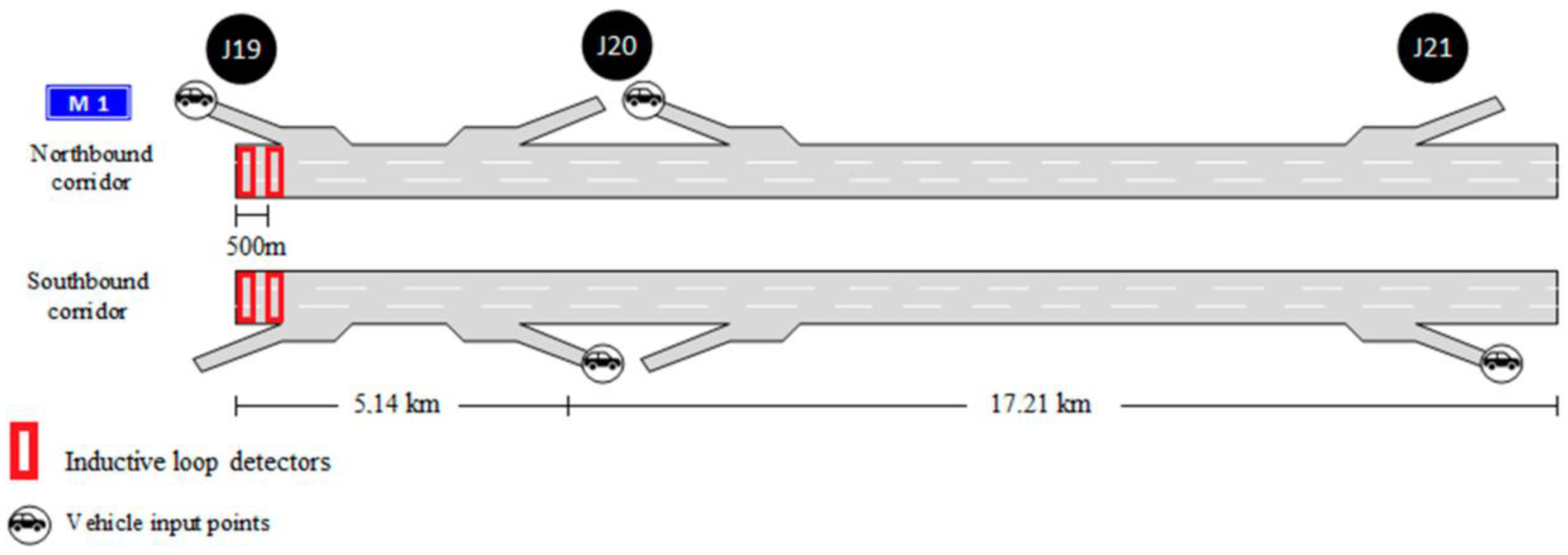
A segment of the three-lane M1 Motorway in the United Kingdom between the cities of Leicester and Rugby was designed in the microsimulation software, consisting of three junctions (J19, J20, and J21). Both directions of the motorway were designed according to real-world geometry. The simulated network was 44.7 km long and contained 4 vehicle input points and 8 merging and diverging areas (See Figure 1 [39]).

Figure 1.
Outline of the simulated motorway network [39].
The real-world mainline corridor of the M1 motorway as well as all the on and off-ramps were equipped with inductive loop detectors approximately every 500 metres. Each set of detectors provided traffic data such as speed, headway, traffic volume, occupancy, and composition for each lane at 1-min intervals [40].
3.2. Data Collection and Traffic Microsimulation Model Validation/Calibration
For a traffic microsimulation model to provide reliable outcomes, it is of utmost importance to be calibrated and validated. Since the final output of the simulation platform is related to safety, a two-stage calibration and validation approach is followed [34,37]. The first stage of the calibration ensures that traffic characteristics such as traffic volume or speed are accurately represented in the simulation, while the second stage of the calibration confirms that the existing safety conditions are simulated efficiently. The developed model was calibrated and validated for traffic conditions between 11:00 and 12:00 am due to data availability. The number of simulations needed to achieve a 95% confidence level for the simulation output was calculated using Equation (1). This equation represents a standard method for estimating the required sample size, which is derived from the normal distribution, where denotes the number of standard deviations corresponding to the desired confidence level (e.g., 95%) [41].
where is the required number of simulation runs, is the sample standard deviation of the simulation output, denotes the Student’s t-statistic for the two-sided error of with degrees of freedom, and represents the allowed error range.
The results showed that 15 simulation runs are sufficient for each calibration and validation stage. The first 800 s of the simulation were used as a warm-up period.
3.2.1. First-Stage Calibration of the Traffic Microsimulation Model
Using historical data (between January 2016 and December 2017) from inductive loop detectors, the input of the simulation was calculated. The dataset was split equally into a calibration and validation dataset. After cleansing and fusing this dataset, the traffic flow values per minute were input in the simulation, along with the speed and time headway distributions for the corresponding time of the day. The performance measures chosen for the first stage of the calibration were the travel time and traffic flow values observed in the field versus the simulated values. To compare the real-world traffic volume measurements to the simulated ones, the Geoffrey E. Havers (GEH) statistic shown in Equation (2) was used:
where stands for the simulated traffic volume and is the observed traffic volume in the real world. For the calibration to be successful, the GEH statistic should be less than 5 for 85% of the compared cases. On the other hand, for travel time calibration and validation, FHWA suggests the direct comparison of the simulated values to the observed ones [42]. According to the same guidelines, the simulated values should be within ±15% of the observed values for more than 85% of the simulated cases. The simulation outputs indicated that 94.18% of the travel time simulated values were within the real-world measurements, and 100% of the traffic volume measurements had a GEH statistic value lower than 5.
3.2.2. Second-Stage Calibration of the Traffic Microsimulation Model
For the second-stage calibration, data collected using the radar-equipped vehicle of Loughborough University were used. Fifteen real-world trips between the simulated junctions on the motorway were conducted between April 2017 and December 2017 with a total duration of 600 min. Using the radar data collected, a Time-To-Collision (TTC) distribution was calculated. TTC is defined as the time that remains until a collision between the leading and following vehicles occurs if they remain on the same path while keeping their current speeds [43]. The TTC equation is presented in Equation (3).
where and indicate the position and the speed of the leading vehicle, and are the position and the speed of the following vehicle, respectively, and is the length of the leading vehicle.
The TTC distribution was calculated from the radar data using an automated algorithm developed in [44]. To complete the second-stage calibration process, a simulated TTC distribution was used. An external code was developed in C++ using the External Driver Model API of PTV VISSIM that could record the TTC values of the simulated vehicles in a data file. The real-world TTC distribution was compared to the TTC distribution from the simulated vehicles using the non-parametric Mann–Whitney statistical test. During the calibration process, the Wiedemann 99 parameter CC3, which is the threshold time gap that a VISSIM vehicle enters the following state, was changed from 8 s to 5 s. After this change, the significance value calculated by the Mann–Whitney test was 0.611, which indicated that the calibration was acceptable. The calibration was also validated using the validation dataset. More details regarding the calibration and validation of the network can be found in [39].
3.3. CAV Driving Behaviour
The External Driver Model API of VISSIM allows the development of a user-defined driver model in C++ programming language. The code is assigned to a specific CAV type in VISSIM. The developed API can access surrounding traffic data such as nearby vehicles’ speeds, accelerations, and distance to the ego vehicle and calculate the state of the vehicle in the next time step. One of the main goals of the developed API is to simulate all the subsystems of the CAV as accurately as possible and address the challenges that are not covered in the existing literature.
3.3.1. Sensing and Perception
The sensing subsystem of a CAV uses a plethora of vehicle sensors, such as radar, lidar, camera, and communication equipment for raw data gathering, while the perception subsystem translates the raw data into useful information about the vehicle and its surroundings. This behaviour is programmed in this paper as follows:
The API-controlled vehicle can scan surrounding traffic up to an infinite range. This assumption was considered unrealistic; therefore, the detection range of the API-controlled vehicle in this study is programmed to represent the scanning range of a typical radar sensor used in motor vehicles (200 m). The raw data initially gathered by the API include 100% accurate data on the surrounding vehicles’ relative speed, distance, lane, and destination. This may not be realistic as real-world sensors are characterised by their operating limits where anomalies are inevitable. Hasch et al. [45] indicate that the typical distance and inaccuracy values of a generic long radar sensor are 0.1 m and 0.1 m/s, respectively, while the manual of a typical automotive long-range radar [46] specifies that the distance and inaccuracy values might reach 0.25 m and 0.14 m/s, respectively. There is a lack of information on how this error in the radar measurements is distributed, and there are significant differences in distance accuracy measurements. According to Zhou et al. [12], a reasonable assumption is that the error follows a normal distribution.
Based on the abovementioned considerations, a first group of scenarios is defined, where the impact of sensor inaccuracies is examined. Since 95% of the observations of a normal distribution fall within the range of two standard deviations from the mean, the standard deviation of the sensor errors with respect to distance and speed measurement pairs (distance s.d and speed s.d.) are 0.05 m and 0.05 m/s, 0.1 m and 0.06 m/s, 0.15 m and 0.07 m/s, and 0.2 m and 0.08 m/s, respectively. These sensor error rates were added to the equations used to control the API-controlled vehicle, which are presented below.
3.3.2. Planning and Control Subsystems
The planning subsystem in a real-world CAV usually includes trajectory planners and behaviour planners, whereas the control subsystem includes the actuators and commands to drive the car.
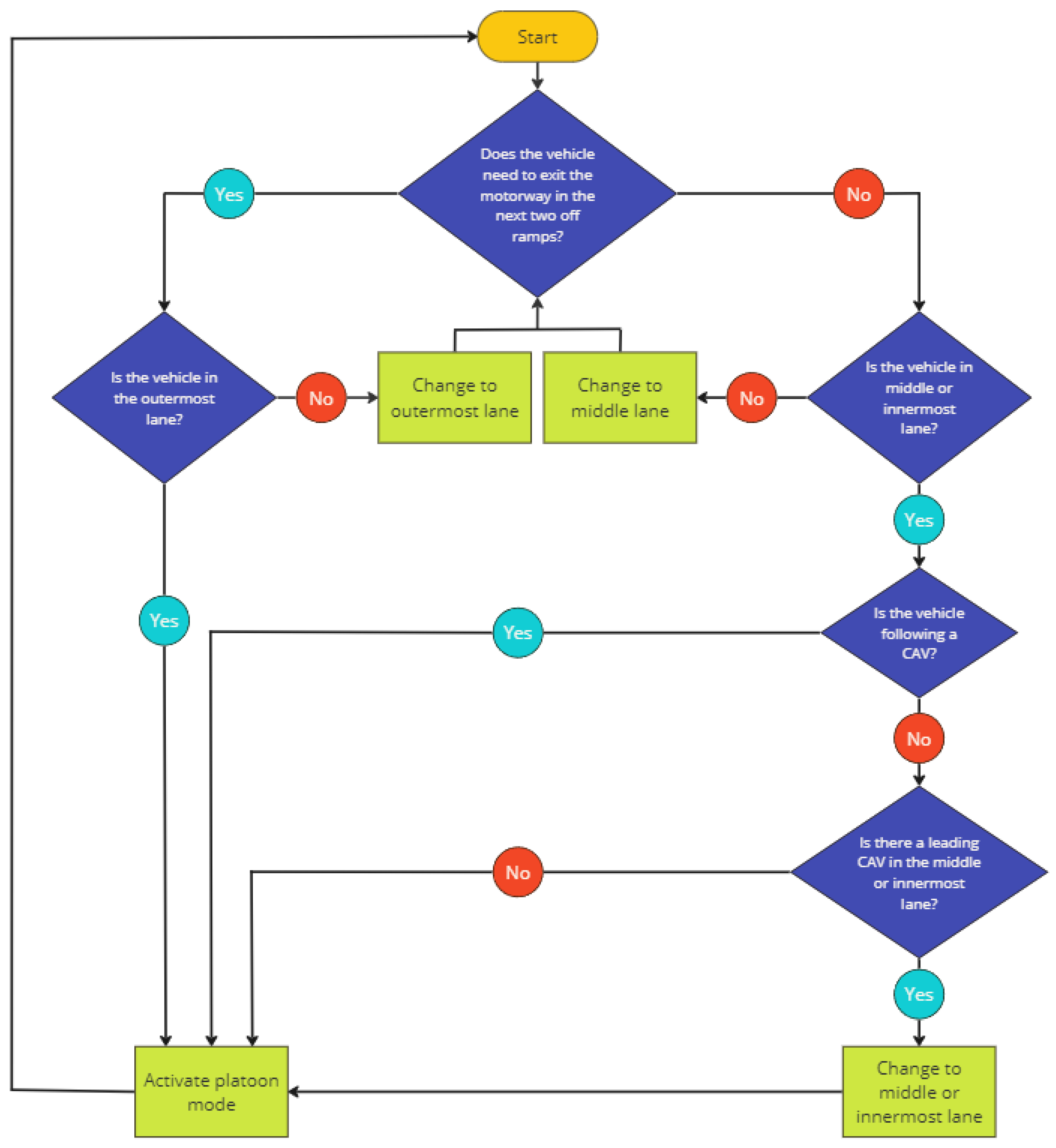
In the developed API, CAVs are programmed to follow a high-level route choice decision-making algorithm. The flowchart of this route choice algorithm is presented in Figure 2. In the route-based decision-making algorithm, a CAV first dynamically selects lanes according to their path planning algorithms, optimising traffic flow and safety. For example, if the destination of the API-controlled vehicle is one of the two upcoming off-ramps on the motorway, the CAV chooses to drive in the outermost lane of the motorway to facilitate a smooth exit. This decision-making process ensures that vehicles intending to exit can do so efficiently without causing disruptions in the inner lanes.

Figure 2.
Flowchart of the high-level CAV route planner.
On the other hand, if the destination is not near, the CAV can select from the remaining lanes of the motorway depending on traffic conditions and other factors such as speed and congestion. For instance, if an API-controlled vehicle is travelling in the middle lane of a three-lane motorway and the preceding vehicle is not a CAV, the system assesses the traffic situation. If a leading CAV is identified in the outermost lane, the system initiates a lane change to the outermost lane. This manoeuvre aims to form a vehicle platoon in the outermost lane, leveraging the benefits of platooning, such as reduced air resistance and improved traffic flow.
This high-level route choice plan results in an even distribution of traffic flow across lanes. By strategically selecting lanes, CAVs contribute to a balanced use of motorway space, preventing congestion in any single lane. Additionally, forming platoons of CAVs with similar destinations enhances traffic efficiency and safety. Platoons can travel at more consistent speeds, maintain shorter following distances safely, and respond to traffic conditions more effectively. Therefore, the dynamic lane selection and platooning behaviour of CAVs based on their path planning and real-time traffic assessments lead to optimised traffic flow, reduced congestion, and improved safety on motorways. This advanced routing and lane-changing strategy ensures that CAVs do not disrupt other vehicles in the network.
All the lane-changing manoeuvres are initiated through the control algorithm of the designed API if a predefined time gap in the target lane is found. The required time gap in this study was 0.6 s from the vehicle upstream and downstream in the target lane. Assuming all road agents are cooperative, the surrounding traffic (both CAVs and human-driven vehicles) can facilitate the lane change process by decelerating if a CAV with an intention to change lanes is identified in an adjacent lane. The start and end times of the lane change, as well as the lane angle and the number of target lanes, are controlled by VISSIM.
Once the CAV is driving in the lane defined by the route planner, the longitudinal constant time gap control algorithm proposed in [39] controls the acceleration, and as a result, the speed of the vehicle. With the simplified vehicle physics in VISSIM, the acceleration of the vehicle is continuously controlled by Equation (4):
where is the speed of the leading vehicle, is the speed of the API-controlled vehicle with the assumption that the desired time gap is not equal to the actual time gap, stands for the desired time gap, and denotes the actual time gap in the current simulation step.
The desired time gap chosen for this study when the API-controlled vehicle was following another CAV was 0.6 s according to previous similar studies [9,10,30]. Subsequently, the upper limits of the acceleration and deceleration were set to 1.5 m/s2 and 2.5 m/s2, respectively, through the GUI of PTV VISSIM following recommendations from Talepbour et al. [47]. The high-level result of the longitudinal control algorithm is the formulation of vehicle platoons.
This study finally evaluates the impact of platoon size on motorway safety. To simplify the experiment, the inter-platoon time gap was set to 3 s according to [48] to allow conventional traffic to navigate. Since three vehicles are required to form a platoon and a platoon size of ten may not be practical in a motorway setting, particularly in a mixed traffic scenario, the platoon sizes tested were three, five, seven, and nine vehicles. These tests were conducted across different market penetration rates, and the safety results were compared to a baseline scenario with no platoon size limit. Other platoon sizes, such as four, six, and eight, were not tested due to the extensive time needed for simulation and the likelihood that their findings would be similar to those already considered. It must be noted that all the investigated platoon size and sensor error scenarios were examined ceteris paribus across different market penetration rates. That means that when the safety impact of sensor error was investigated, the platoon size was not considered in the experiment. Five discrete market penetration rates (0%, 25%, 50%, 75%, and 100%) were selected for evaluation.
3.4. Traffic Conflict Identification and Statistical Modelling Method
To evaluate the safety impact of CAVs, the SSAM was employed. SSAM is a tool developed and validated by FHWA that utilises automated algorithms to identify traffic conflicts from vehicle trajectory files produced by VISSIM [15]. The SSAM processes one simulation time step at a time and checks for traffic conflicts using predefined TTC and Post Encroachment Time (PET) threshold values. The default values for TTC and PET were 1.5 s and 5.0 s, respectively [15]. While processing the vehicle trajectory files, the SSAM projects the vehicles’ future positions for up to the duration of the predefined TTC value. If a vehicle overlap is identified in this way, this pair of vehicles is recorded in the SSAM output file.
Along with the identification of the conflicting vehicles, the SSAM provides data about the conflict itself, such as the conflict type (i.e., rear-end and lane change), the simulation time when the conflict occurred, and the coordinates of the location of the conflict. In this paper, using the location of the conflict and data collected through the data collection points placed in the VISSIM network, traffic conflict counts were matched to the corresponding traffic-related measurements produced by VISSIM. Traffic data collection points were placed in VISSIM at every 500 metres, and two consequent traffic data collection points in VISSIM defined a motorway segment. The result of this process was a dataset containing the variables presented in Table 1, along with their descriptive statistics.

Table 1.
Summary statistics of conflict dataset.
To model segment-based traffic conflicts, a Bayesian hierarchical negative binomial model that takes into account spatial autocorrelation was employed. The presence of spatial autocorrelation with respect to traffic conflicts by segment was confirmed by the Moran’s I statistic, which measures the similarities in observations across space. The Moran’s I statistic was calculated through Equation (5), and its value for the dataset of this paper was found to be 0.40, indicating the presence of spatial autocorrelation.
where is the number of spatial units indexed by and ; the variable of interest, and is its mean; a spatial weights matrix, where is 1 if the and sections are adjacent or 0 otherwise; and is the sum of all .
The formulation of the Bayesian hierarchical negative binomial model employed is presented below:
where are the parameters of the negative binomial distribution, is the exposure variable, denotes the coefficients of the explanatory variable (), represents the random spatial effects, represents the unobserved heterogeneity, denotes the random intercept at the segment level, and is the observed number of conflicts, which follows a negative binomial distribution. always follows a highly non-informative normal distribution with a mean of zero, and UH is assumed to follow a normal distribution, , where is the precision (i.e., 1/variance) with a gamma prior distribution Ga (0.5, 0.0005). The effect of spatial correlation is included as a conditional autoregressive prior with , with , being defined by the following equations:
where is assumed to follow a gamma prior distribution with Ga (0.5, 0.0005). The Bayesian hierarchical model can be estimated using Bayesian inference using Gibb’s sampling (WINBUGS) by employing the Markov chain Monte Carlo method. The goodness-of-fit statistic, i.e., the Deviance Information Criterion (DIC), which is used to compare the fit of models estimated on a full Bayesian inference approach, was employed (see Equation (10)). The most parsimonious model is defined as the model that accomplishes a good level of explanation of the data using the least explanatory variables possible. This model will have the smallest DIC value among all the possible models [49]. The mathematical formulation describing the DIC is presented below:
where is the deviance of the θ posterior mean of the model parameters, is the effective number of parameters in the model, and denotes the posterior mean of the deviance, .
4. Findings and Discussion
For each defined scenario, 15 simulations were conducted with different random seeds. After each simulation run, the vehicle trajectory file obtained from PTV VISSIM was processed by the SSAM, and the traffic conflicts were calculated. Only rear-end and lane-changing conflicts were taken into consideration according to [50]. The results regarding the route-based decision-making algorithm are presented in Figure 3. It can be seen that the route-based decision-making algorithm (orange) has a positive safety effect; it reduces the total number of traffic conflicts by 18.56%, 18.99%, 19.23%, and 25% in the 25%, 50%, 75%, and 100% market penetration rate scenarios, respectively. It must be emphasised that the percent conflict reduction increases as the market penetration rate increases. This is undoubtedly because as the percentage of CAVs in the motorway increases, they form platoons that travel in the lane that corresponds to their destination, ultimately reducing the sheer amount of unnecessary lane changes that could potentially lead to traffic conflicts.
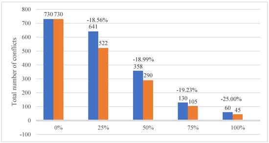
Figure 3.
Total number of conflict reduction due to the route-based decision-making algorithm.
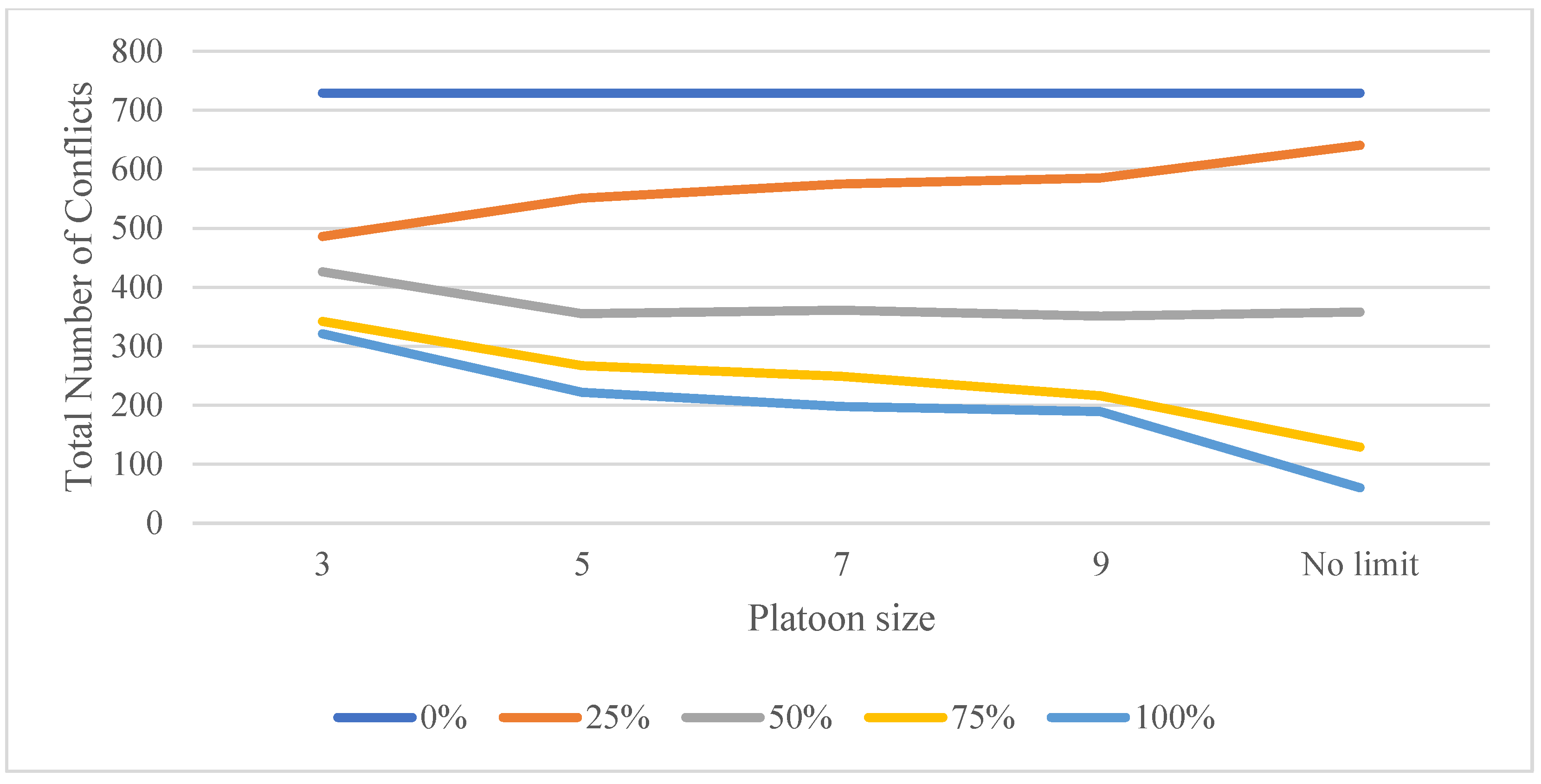
The results regarding the safety impacts of platoon size for all the predefined market penetration rates are presented in Figure 4. If the market penetration rate is examined alone, it is obvious that CAVs provide a significant benefit in terms of reducing the number of simulated conflicts. However, when examining the impact of platoon size within the same market penetration rate, the results provide an interesting insight.
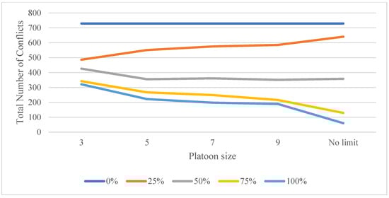
Figure 4.
Number of total conflicts (15 simulation runs per market penetration rate and platoon size).
In more detail, at the 25% market penetration rate, an increase in the number of conflicts is observed as the platoon size increases. This result is surprising at first, but it can be explained as follows: after observing the simulation environment, this increase in conflicts is likely due to the fact that human-driven vehicles (75% of all traffic) can manoeuvre more safely when the platoon size is 3 than when it is 5 or higher. In addition, a relatively long platoon may cause disruptions in traffic dynamics such as restraining human-driven vehicles to make lane change manoeuvres, especially near the diverging areas of the motorway. A larger increase is noticeable when the platoon size increases from 3 to 5 than when the platoon size changes from 5 to 7 and 9, consecutively. This can be explained by the fact that in this market penetration rate (25%), the formation of platoons with five or more vehicles is a rare occasion due to the small relative numbers; hence, the safety results were similar.
At the 50% market penetration rate, a safety benefit was observed when the platoon size increased from three vehicles to five vehicles. However, there was no statistically significant difference in simulated conflicts between platoon sizes five, seven, and nine and no platoon size limit scenarios. This observation was confirmed using the Kruskal–Wallis statistical test, which compares samples to determine whether they originate from the same distribution. The p-value of the statistic of the Kruskal–Wallis test was 0.911, which indicates that the difference in the number of conflicts between these scenarios was not significant.
When the CAV market penetration rate reaches 75% and 100%, a steady safety improvement is observed as the platoon size increases, which reaches 91.77% at the 100% market penetration rate of the no platoon size limit scenario. This implies that, when the CAV market penetration rate reaches 75% and higher, the impact of the platoon in the motorway in terms of safety is immense. As most vehicles are organised in vehicle platoons, the occupancy rate of the motorway is lower, creating free space for manoeuvring, ultimately reducing the number of vehicle interactions that could potentially be dangerous.
These findings could be proven useful to network owners and policymakers regarding the real-world CAV platoon implementation strategy on motorways. According to Figure 4, there is not a single optimal platoon size that would provide the greatest safety benefit. The optimal platoon size depends on the CAV market penetration rate. For example, platoon size 3 provides a greater safety benefit than the other platoon sizes in low CAV market penetration rates (25%), whereas a platoon size with five or more vehicles can provide a larger safety benefit as the CAV market penetration rate increases.
The safety impact of the sensor error per market penetration rate is presented in Table 2. The safety benefit of CAVs is obvious as the market penetration rate increases throughout all sensor error values. However, the differences in simulated conflicts within the same market penetration rate under different sensor error scenarios are statistically insignificant. To confirm this observation, four Kruskal–Wallis tests were performed for the 25, 50, 75, and 100% market penetration rates. The p-values of the tests were 0.65, 0.51, 0.42, and 0.40, respectively, and indicated that the null hypothesis that the samples originate from the same distribution could be retained. It is worthwhile to note that the sensor error is assumed to follow a Gaussian distribution () with a small standard deviation compared to the average measured values. For example, in a formulated platoon that is driving at a speed of 28 m/s (100 km/h) and a time gap of 0.6 s (17.8 metres), a sensor error of 0.1 m for the distance measurement and 0.1 m/s for the speed measurement of the leading vehicle might not be sufficient to cause additional traffic conflicts. However, the proposed methodological framework is transferable, and any given sensor error rate can be tested if it is deemed more appropriate.
Table 2.
Total number of conflicts per market penetration rate and sensor error standard deviation.
Finally, the posterior estimates for the significant variables of the statistical model are presented in Table 3.
Table 3.
Estimation results for the traffic conflict Bayesian hierarchical model.
As can be seen, the posterior mean for the standard deviation of spatial correlation (SC) is 0.73 and is statistically significant at the 95% confidence level, confirming that traffic conflicts are spatially correlated among neighbouring motorway segments. However, the value is low compared to other studies employing this method [16]. Similarly, the standard deviation of the unobserved heterogeneity (UH) and the random intercept term at the segment level (SL) are also statistically significant, indicating similarities in the number of conflicts coming from the same segment.
The effect of the CAV market penetration rate is negative, meaning that as the market penetration rate increases, the logarithm of the conflicts decreases, which is in line with the simulation results presented above. The standard deviation of speeds between lanes seems to affect the number of conflicts per segment. Even though this result cannot be directly compared to the existing literature, the standard deviation of speeds has been proven to have a positive coefficient when used for the modelling of accidents [51,52]. In these results, the standard deviation of speeds between lanes has a positive coefficient as well, which can be interpreted as follows: as the standard deviation of speeds between lanes increases, the logarithm of traffic conflicts increases. This result seems logical as speed differences across lanes lead to more overtakes in adjacent lanes, which increases the possibility for a potentially dangerous incident to occur.
The lack of a dummy variable describing whether the segment is a merging or diverging area from the list of significant variables is surprising if one considers the conclusions of the existing literature [39]. The merging areas of the motorway are conflict hotspots where vehicles are using the acceleration lane to merge in terms of speed and traffic flow to the motorway. Inevitably, there are larger speed differences between lanes in these areas as the accelerating vehicles start from slower speeds to reach the average speed of the motorway. Hence, it is considered that the effect of the merging area is captured by the standard deviation of speeds between lanes.
5. Conclusions
The evidence regarding the potential safety benefits of CAVs has been limited due to a lack of real-world data. The existing literature has focused on a few CAV driving characteristics and has not addressed fundamental operational and technological challenges or explained the underlying factors affecting CAV safety in depth. This paper addressed this knowledge gap by presenting a traffic microsimulation platform that includes sensor error according to accuracy values found in the literature, a route-based decision-making algorithm for CAVs (i.e., path choice), and platoon size in the analysis to evaluate their safety impact. It must be emphasised that due to the lack of CAV data, the aforementioned CAV algorithms could not be calibrated. The safety impact of CAVs was statistically modelled in terms of traffic conflicts using a hierarchical Bayesian negative binomial model that considered spatial autocorrelation and unobserved heterogeneity.
The simulation results indicate that the inaccuracy rates of real-world automotive radars do not significantly affect the number of simulated traffic conflicts. This supports the reliability of current radar technologies in CAVs. Additionally, this study reveals that there is no single optimal platoon size for all market penetration rates. Smaller platoons (three vehicles) are more effective in reducing conflicts by 33.33% at lower market penetration rates (25%). Conversely, larger platoons (five or more vehicles) offer better safety benefits at higher market penetration rates (50%, 75%, and 100%), with an average conflict reduction of 63.30%. This finding suggests that adaptive platoon sizes could enhance motorway safety during the transition to widespread CAV usage.
As the market penetration rate of CAVs increases, the total number of traffic conflicts decreases significantly. This reduction is attributed to the formation of vehicle platoons that minimise unnecessary lane changes and optimise traffic flow. Moreover, this study identifies that a higher standard deviation of speeds between lanes increases the number of traffic conflicts. This underscores the importance of redesigning motorway areas with high-speed variability, such as merging zones, to improve safety.
The findings provide valuable insights for network operators, policymakers, and legislative bodies. Implementing appropriate platoon sizes at various stages of CAV market penetration can significantly enhance motorway safety. For instance, smaller platoons are more effective at reducing conflicts at lower market penetration rates, while larger platoons offer greater safety benefits as penetration rates increase. Additionally, addressing speed variability in critical areas, such as merging zones, can further reduce traffic conflicts and enhance overall traffic flow stability.
However, several limitations should be noted. First, the TTC distribution was calculated from instrumented data collected with a limited number of trips and drivers. A larger and more representative dataset could produce more reliable real-world TTC distributions. Second, this study relies on traffic flow data collected between 11 and 12 AM. The impact of CAVs during peak hours could be significantly different and needs further investigation. Third, in the platoon size scenarios, CAVs were assumed to have 100% compliance with the given platoon size, and only one size was tested per scenario. Additionally, only rear-end platoon joining was considered, and it was assumed that all CAVs could form platoons with all the other CAVs, which may not be true due to differences in underlying hardware and software.
Nonetheless, using the methodology presented in this study, more complex scenarios can be evaluated in future work. This includes the real-time re-routing of CAV fleets in response to motorway disruptions and integrating existing traffic management systems like variable speed limits and ramp metering to evaluate their combined impact on CAV safety.
Author Contributions
Conceptualisation, A.P., M.I. and M.Q., methodology, A.P. and M.I.; writing—original draft preparation, A.P. and Y.F.; supervision, M.Q. All authors have read and agreed to the published version of the manuscript.
Funding
This research received no external funding.
Data Availability Statement
Dataset available on request from the authors.
Conflicts of Interest
Author Alkis Papadoulis was employed by the company Aimsun. Author Marianna Imprialou was employed by the company Ernst & Young. The remaining authors declare that the research was conducted in the absence of any commercial or financial relationships that could be construed as a potential conflict of interest.
References
- Fagnant, D.J.; Kockelman, K. Preparing a Nation for Autonomous Vehicles: Opportunities, Barriers and Policy Recommendations. Transp. Res. A Policy Pract. 2015, 77, 167–181. [Google Scholar] [CrossRef]
- Singh, S. Critical Reasons for Crashes Investigated in the National Motor Vehicle Crash Causation Survey. (Traffic Safety Facts Crash•Stats); National Highway Traffic Safety Administration: Washington, DC, USA, 2015; pp. 2–3. [Google Scholar]
- Kalra, N.; Paddock, S.M. Driving to Safety: How Many Miles of Driving Would It Take to Demonstrate Autonomous Vehicle Reliability? Transp. Res. A Policy Pract. 2016, 94, 182–193. [Google Scholar] [CrossRef]
- Monasterio, F.; Nguyen, A.; Lauber, J.; Boada, M.; Boada, B. Event-Triggered Robust Path Tracking Control Considering Roll Stability Under Network-Induced Delays for Autonomous Vehicles. IEEE Trans. Intell. Transp. Syst. 2023, 24, 14743–14756. [Google Scholar] [CrossRef]
- Dong, C.Y.; Liu, Y.J.; Wang, H.; Ni, D.H.; Li, Y. Modelling Lane-Changing Behavior Based on a Joint Neural Network. Machines 2022, 10, 109. [Google Scholar] [CrossRef]
- Wang, Y.B.; Wang, L.; Guo, J.Q.; Ioannis, P.; Papageorgiou, M.; Wang, F.Y.; Bertini, R.; Hua, W.; Yang, Q.M. Ego-Efficient Lane Changes of Connected and Automated Vehicles with Impacts on Traffic Flow. Transp. Res. Part C Emerg. Technol. 2022, 138, 103478. [Google Scholar] [CrossRef]
- Du, R.J.; Chen, S.K.; Li, Y.J.; Dong, J.Q.; Ha, P.; Labi, S. A Cooperative Control Framework for CAV Lane Change in a Mixed Traffic Environment. In Proceedings of the Transportation Research Board, Washington DC, USA, 9–13 January 2021. [Google Scholar]
- Jeong, E.; Oh, C.; Lee, S. Is Vehicle Automation Enough to Prevent Crashes? Role of Traffic Operations in Automated Driving Environments for Traffic Safety. Accid. Anal. Prev. 2017, 104, 115–124. [Google Scholar] [CrossRef] [PubMed]
- ATKINS. Research on the Impacts of Connected and Autonomous Vehicles (CAVs) on Traffic Flow. 2016. Available online: https://trid.trb.org/View/1448450 (accessed on 10 October 2019).
- Rahman, M.S.; Abdel-Aty, M. Longitudinal Safety Evaluation of Connected Vehicles’ Platooning on Expressways. Accid. Anal. Prev. 2017, 117, 381–391. [Google Scholar] [CrossRef] [PubMed]
- Papadoulis, A.; Quddus, M.; Imprialou, M. Estimating the Corridor-Level Safety Impact of Connected and Autonomous Vehicles. In Proceedings of the Transportation Research Board, Washington DC, USA, 7–11 January 2018. [Google Scholar]
- Zhou, Y.; Ahn, S.; Chitturi, M.; Noyce, D.A. Rolling Horizon Stochastic Optimal Control Strategy for ACC and CACC under Uncertainty. Transp. Res. Part C Emerg. Technol. 2017, 83, 61–76. [Google Scholar] [CrossRef]
- Bernardini, D.; Bemporad, A. Scenario-Based Model Predictive Control of Stochastic Constrained Linear Systems. In Proceedings of the 48h IEEE Conference on Decision and Control (CDC) Held Jointly with 2009 28th Chinese Control Conference, Shanghai, China, 15–18 December 2009; pp. 6333–6338. [Google Scholar]
- Wiseman, Y. Autonomous vehicles. Encycl. Inf. Sci. Technol. 2020, 1, 1–11. [Google Scholar]
- Gettman, D.; Pu, L.; Sayed, T.; Shelby, S.G. Surrogate Safety Assessment Model and Validation: Final Report; Turner-Fairbank Highway Research Center: McLean, VA, USA, 2008; p. FHWA-HRT-08-051. [Google Scholar]
- Quddus, M. Modelling Area-Wide Count Outcomes with Spatial Correlation and Heterogeneity: An Analysis of London Crash Data. Accid. Anal. Prev. 2008, 40, 1486–1497. [Google Scholar] [CrossRef]
- Imprialou, M.; Quddus, M.; Pitfield, D.E.; Lord, D. Re-Visiting Crash-Speed Relationships: A New Perspective in Crash Modelling. Accid. Anal. Prev. 2016, 86, 173–185. [Google Scholar] [CrossRef] [PubMed]
- Dosovitskiy, A.; Ros, G.; Codevilla, F.; Lopez, A.; Koltun, V. CARLA: An Open Urban Driving Simulator. In Proceedings of the 1st Annual Conference on Robot Learning, Mountain View, CA, USA, 13–15 November 2017; pp. 1–16. [Google Scholar]
- Feng, Y.X.; Ye, Q.M.; Angeloudis, P. Rapid Procedural Generation of Real World Environments for Autonomous Vehicle Testing. In Proceedings of the ICRA 2023 Workshop on Bridging the Lab-to-Real Gap: Conversations with Academia, Industry, and Government, London, UK, 29 May–2 June 2023. [Google Scholar]
- Kato, S.; Tokunaga, S.; Maruyama, Y.; Maeda, S.; Hirabayashi, M.; Kitsukawa, Y.; Monrroy, A.; Ando, T.; Fujii, T.; Azumu, T. Autoware on Board: Enabling Autonomous Vehicles with Embedded Systems. In Proceedings of the 2018 ACM/IEEE 9th International Conference on Cyber-Physical Systems (ICCPS), Porto, Portugal, 11–13 April 2018; pp. 287–296. [Google Scholar]
- van Noort, M.; van Arem, B.; Park, B. MOBYSIM: An Integrated Traffic Simulation Platform. In Proceedings of the 13th International IEEE Conference on Intelligent Transportation Systems, Funchal, Portugal, 19–22 September 2010. [Google Scholar]
- Li, Z.; Chitturi, M.V.; Zheng, D.; Bill, A.R.; Noyce, D.A. Modeling Reservation-Based Autonomous Intersection Control in VISSIM Modeling Reservation-Based Autonomous Intersection Control in VISSIM. Transp. Res. Rec. 2013, 2381, 81–90. [Google Scholar] [CrossRef]
- Li, H.Z.; Roncoli, C.; Zhao, W.M.; Ju, Y.F. Assessing the Impact of CAV Driving Strategies on Mixed Traffic on the Ring Road and Freeway. Sustainability 2024, 16, 3179. [Google Scholar] [CrossRef]
- Hou, G.Y. Evaluating Efficiency and Safety of Mixed Traffic with Connected and Autonomous Vehicles in Adverse Weather. Sustainability 2023, 15, 3138. [Google Scholar] [CrossRef]
- Liang, J.H.; Li, Y.J.; Yin, G.D.; Xu, L.W.; Lu, Y.B.; Feng, J.W.; Shen, T.; Cai, G.S. A MAS-Based Hierarchical Architecture for the Cooperation Control of Connected and Automated Vehicles. IEEE Trans. Veh. Technol. 2022, 72, 1559–1573. [Google Scholar] [CrossRef]
- Zhou, Z.; Li, L.H.; Qu, X.; Ran, B. An autonomous platoon formation strategy to optimize CAV car-following stability under periodic disturbance. Phys. A Stat. Mech. Appl. 2023, 626, 129096. [Google Scholar] [CrossRef]
- Liang, J.H.; Tian, Q.Y.; Feng, J.W.; Pi, D.W.; Yin, G.D. A Polytopic Model-Based Robust Predictive Control Scheme for Path Tracking of Autonomous Vehicles. IEEE Trans. Intell. Vehicl. 2024, 9, 3928–3939. [Google Scholar] [CrossRef]
- Roncoli, C.; Papageorgiou, M.; Papamichail, I. Motorway Traffic Flow Optimisation in Presence of Vehicle Automation and Communication Systems. Comput. Methods Appl. Sci. 2015, 38, 1–16. [Google Scholar]
- Park, H.; Smith, B. Investigating Benefits of IntellidriveSM in Freeway Operations-Lane Changing Advisory Case Study. J. Transp. Eng. 2012, 138, 1113–1122. [Google Scholar] [CrossRef]
- Stanek, D.; Huang, E.; Milam, R.; Wang, Y. Measuring Autonomous Vehicle Impacts on Congested Networks Using Simulation. In Proceedings of the Transportation Research Board 97th Annual Meeting, Washington, DC, USA, 7–11 January 2018; p. 728. [Google Scholar]
- Jiang, Y.; Li, S.; Shamo, D.E. A Platoon-Based Traffic Signal Timing Algorithm for Major-Minor Intersection Types. Transp. Res. B Methodol. 2006, 40, 543–562. [Google Scholar] [CrossRef]
- Mouhagir, H.; Cherfaoui, V.; Talj, R.; Aioun, F.; Guillemard, F. Trajectory Planning for Autonomous Vehicle in Uncertain Environment Using Evidential Grid. IFAC-PapersOnLine 2017, 50, 12545–12550. [Google Scholar] [CrossRef]
- Morando, M.M.; Truong, L.T.; Vu, H.L. Investigating Safety Impacts of Autonomous Vehicles Using Traffic Micro-Simulation. In Proceedings of the Australasian Transport Research Forum, Auckland, New Zealand, 27–29 November 2017; pp. 1–6. [Google Scholar]
- Fan, R.; Wang, W.; Liu, P.; Yu, H. Using VISSIM Simulation Model and Surrogate Safety Assessment Model for Estimating Field Measured Traffic Conflicts at Freeway Merge Areas. IET Intell. Transp. Syst. 2013, 7, 68–77. [Google Scholar] [CrossRef]
- Lord, D.; Mannering, F. The Statistical Analysis of Crash-Frequency Data: A Review and Assessment of Methodological Alternatives. Transp. Res. A Policy Pract. 2010, 44, 291–305. [Google Scholar] [CrossRef]
- Besag, J.; York, J.; Mollié, A. Bayesian Image Restoration with Two Applications in Spatial Statistics. Ann. Inst. Stat. Math. 1991, 43, 1–20. [Google Scholar] [CrossRef]
- Huang, F.; Liu, P.; Yu, H.; Wang, W. Identifying If VISSIM Simulation Model and SSAM Provide Reasonable Estimates for Field Measured Traffic Conflicts at Signalized Intersections. Accid. Anal. Prev. 2013, 50, 1014–1024. [Google Scholar] [CrossRef] [PubMed]
- Gomes, G.; May, A.; Horowitz, R. Congested Freeway Microsimulation Using VISSIM. Transp. Res. Rec. 2004, 1876, 71–81. [Google Scholar] [CrossRef]
- Papadoulis, A.; Quddus, M.; Imprialou, M. Evaluating the Safety Impact of Connected and Autonomous Vehicles on Motorways. Accid. Anal. Prev. 2019, 124, 12–22. [Google Scholar] [CrossRef] [PubMed]
- MacDonald, M. MIDAS Database. Available online: https://www.midas-data.org.uk/ (accessed on 14 November 2019).
- Shahdah, U.; Saccomanno, F.; Persaud, B. Application of Traffic Microsimulation for Evaluating Safety Performance of Urban Signalized Intersections. Transp. Res. Part C Emerg. Technol. 2015, 60, 96–104. [Google Scholar] [CrossRef]
- Dowling, R.; Skabardonis, A.; Alexiadis, V. Traffic Analysis Toolbox Volume III: Guidelines for Applying Traffic Microsimulation Modeling Software; Rep. No. FHWA-HRT-04-040, U.S. DOT; Federal Highway Administration: Washington, DC, USA, 2004; Volume III, p. 146. [Google Scholar]
- Hayward, J.C. Near Miss Determination through Use of a Scale of Danger. Report No. TTSC 7115. 1972. Available online: https://onlinepubs.trb.org/Onlinepubs/hrr/1972/384/384-004.pdf (accessed on 23 November 2019).
- Formosa, N.; Quddus, M.; Ison, S.; Abdel-Aty, M.; Yuan, J. Predicting Real-Time Traffic Conflicts Using Deep Learning. Accid. Anal. Prev. 2020, 136, 105429. [Google Scholar] [CrossRef]
- Hasch, J.; Topak, E.; Schnabel, R.; Zwick, T.; Weigel, R.; Waldschmidt, C. Millimeter-Wave Technology for Automotive Radar Sensors in the 77 GHz Frequency Band. IEEE Trans. Microw. Theory Tech. 2012, 60, 845–860. [Google Scholar] [CrossRef]
- Continental. ARS 30X/-2/-2C/-2T/-21 Long Range Radar Specifications. 2012. Available online: https://freecon.co.kr/?act=common.download_goods&fseq=588&u=manual (accessed on 10 December 2019).
- Talebpour, A.; Mahmassani, H.S. Influence of Connected and Autonomous Vehicles on Traffic Flow Stability and Throughput. Transp. Res. Part C Emerg. Technol. 2016, 71, 143–163. [Google Scholar] [CrossRef]
- Varaiya, P. Smart Cars on Smart Roads: Problems of Control. IEEE Trans. Intell. Transp. Syst. 1993, 38, 195–207. [Google Scholar] [CrossRef]
- Spiegelhalter, D.J.; Best, N.G.; Carlin, B.P. Bayesian Deviance with Discussion JRSSB 2002. Appl. Stat. 2002, 46, 261–304. [Google Scholar]
- Pu, L.; Joshi, R. Surrogate Safety Assessment Model (SSAM): Software User Manual; Turner-Fairbank Highway Research Center: McLean, VA, USA, 2008. [Google Scholar]
- Taylor, M.C.; Lynam, D.A.; Baruya, A. The Effects of Drivers’ Speed on the Frequency of Road Accidents Prepared for Road Safety Division; Transport Research Laboratory: Crowthorne, UK, 2000. [Google Scholar]
- Quddus, M. Exploring the Relationship Between Average Speed, Speed Variation, and Accident Rates Using Spatial Statistical Models and GIS. J. Transp. Saf. Secur. 2013, 5, 27–45. [Google Scholar] [CrossRef]

Disclaimer/Publisher’s Note: The statements, opinions and data contained in all publications are solely those of the individual author(s) and contributor(s) and not of MDPI and/or the editor(s). MDPI and/or the editor(s) disclaim responsibility for any injury to people or property resulting from any ideas, methods, instructions or products referred to in the content. |
© 2024 by the authors. Licensee MDPI, Basel, Switzerland. This article is an open access article distributed under the terms and conditions of the Creative Commons Attribution (CC BY) license (https://creativecommons.org/licenses/by/4.0/).