A Novel Double Closed Loop Control of Temperature and Rotational Speed for Integrated Multi-Parameter Hydro-Viscous Speed Control System (HSCS)

Abstract

Hydro-viscous clutch has already become an inevitable choice for special vehicle transmission in the present and future. As a nonlinear system with a large hysteresis loop, its speed control performance is affected by input rotational speed, lubricating oil temperature, lubrication pressure, and other factors. The traditional control method cannot adjust the temperature and rotational speed, which will lead to problems of narrow speed range, poor rotational speed stability, and large dynamic load impact. In order to solve the above problems, this paper studies the control method of an integrated multi-parameter hydro-viscous speed control system (HSCS) in a controlled environment. Through the mechanism analysis of the law of HSCS, the influence law of speed and temperature during the system operation is found. The temperature closed loop based on model predictive control (MPC) is introduced to control the rotational speed, and then the traditional PID control results are compensated according to the speed closed loop. Next, a novel double closed loop control method of temperature and rotational speed for HSCS is formed. Finally, the simulating verification is carried out. Compared with the traditional control method, the design method in this paper can adjust the control parameters according to the temperature of the lubricating oil and the input rotational speed and effectively expand the domain of HSCS and the speed control stability. The effective transmission ratio is extended to 0.2~0.8, and the hydro-viscous torque and speed fluctuation under the engine rotational speed fluctuation are reduced by more than 30%. The novel control method of HSCS designed in this paper can effectively improve the influence of input rotational speed and lubricating oil temperature on the speed control performance of HSCS and can be widely used in nonlinear HSCS such as hydro-viscous clutch.

1. Introduction

Hydro-viscous clutch has the advantages of compact structure, lightweight, high efficiency, and stepless speed control. Therefore, the technology of HSCS has become an inevitable choice for special vehicle transmission from the present to the future [1,2]. Because the hydro-viscous clutch is a nonlinear system with a large hysteresis loop, its speed control performance is affected by input rotational speed, lubricating oil temperature, lubricating pressure, and other factors. In addition, there are some nonlinear factors in the proportional valve. Therefore, the HSCS is a multi-parameter, strong coupling, and strong nonlinear hydraulic transmission system. The main interference factors are the fluctuation of engine rotational speed and the change in lubricating oil temperature [3,4,5,6], which lead to the problems of narrow speed control range, large fluctuation of fan rotational speed, and large impact on the torque of transmission shaft in the speed control process.

In addition, HSCS is a nonlinear system. The key to the rotational speed control loop is to overcome serious nonlinear problems such as large hysteresis, large dead zone, and time-varying parameters of the hydro-viscous clutch [7,8,9]. It is necessary to dynamically change the control parameters according to the changes in the model and working conditions [10,11]. Therefore, the design of HSCS needs to consider a variety of nonlinear control schemes, especially the hysteresis nonlinear problem [12,13].

In order to further improve the control characteristics of the HSCS, more researchers are focusing on the design of control methods [14,15]. Yin XiuXing et al. used the traditional PID closed loop control method [16]. Jahmeerbacus et al. proposed a control system based on the fuzzy logic strategy [17]. Kastrevc et al. used the fuzzy PID controller to improve the pressure control performance of the pump control system, and the simulation verified the obvious robustness of the fuzzy PID controller [18]. Yi Ye et al. proposed an improved particle swarm optimization algorithm to search the PID controller gain of the nonlinear hydraulic system to solve nonlinear problems such as dead zone, saturation, flow coefficient, and friction in the system [19]. Haibo Liang et al. proposed an improved genetic algorithm to optimize the fuzzy PID controller, which improved the performance of the nonlinear hydraulic system in terms of speed, stability, and robustness [20]. Yuan Ji et al. proposed a high-precision pressure tracking method with an accurate performance boundary. Combining adaptive robust control with a prescribed performance mechanism, they proposed a constrained adaptive robust controller [21]. Junting Lu et al. introduced an additional variable to represent the nonlinearity of the system in the frequency characteristic model of the hydraulic system and proposed a variable parameter feedforward control method with better phase characteristics and higher tracking accuracy [22]. Yanhe Song et al. studied the nonlinear dynamic behavior of a pressure servo valve-controlled cylinder system (PSVCS) and obtained the influence of key parameters on nonlinear self-excited behavior [23]. Qixin Zhu designed a compound control method combining sliding mode control (SMC) and model-based linear extended state observer (MLESO). Simulations show that the method has a good control effect. The maximum error is 0.101 mm under different working conditions, and the maximum error change is 36.5% [24]. Zhihua Chen designed a predictive tracking controller based on a fuzzy model and a novel gait transition level control framework based on a flexible gait planner (FGP) and gait feedback regulator (GFR) with behavior rules and successfully applied it to the walking control framework of a six-wheeled robot [25,26].Kaixian Ba proposed a bionic perception and transmission neural device for the leg hydraulic nonlinear drive system, It can carry out passive control in the presence of nonlinear hydraulic system [27]. Based on the analysis of existing methods, the following problems were identified:

• The traditional PID control method commonly used in the HSCS cannot change the PID control parameters according to the working conditions and adjust the system according to the influence factors such as engine rotational speed fluctuation and lubricating oil temperature change. Moreover, rotational speed fluctuations of the engine and lubricating oil temperature are polytropic and lack variation. Therefore, it is difficult to manually develop control parameters to adjust.
• Although the existing fuzzy control and other methods can compensate for the influence of rotational speed fluctuation, pressure, and other factors, the influence of lubricating oil temperature in the HSCS is very complicated. There is no way to carry out traditional mathematical modeling, and it is impossible to adjust the input rotational speed according to the change in oil temperature, which will lead to the continuous rise of oil temperature and affect the working performance of the system.

Through investigation, the current mature control methods have a low compensation progress for the impact of rotational speed fluctuation and lubricating oil temperature change and cannot be adjusted at the same time, which will eventually lead to the narrowing of the speed control domain of the HSCS, the increase in fan rotational speed fluctuation, and the torque impact on the transmission shaft.

To give full play to the advantages of HSCS, expand its effective speed control domain, and improve its speed control performance, this paper studies the double closedloop control method of HSCS based on engine rotational speed fluctuation and lubricating oil temperature change. Innovations are as follows:

• Aiming at the influence of lubricating oil temperature on the system, considering that the HSCS has the characteristics of nonlinearity, time-varying, strong coupling, and uncertainty, it is difficult to obtain an accurate mathematical model. The temperature closed loop based on model predictive control (MPC) is introduced to control the rotational speed. By compensating for the influence of oil temperature change on the HSCS, the system control accuracy is improved.
• Aiming at the influence of the input rotational speed on the system, the closed loop control structure based on the revolution speed is used, and the output of the equal ratio inverse model built by the neural network is used as the feedforward compensation. The adaptive algorithm is used to adjust the PID control parameters to realize the output rotational speed of the hydro-viscous to follow the desired rotational speed change, and the nonlinear large hysteresis characteristics of HSCS are transformed into an approximate linear relationship, thereby improving the domain of HSCS.

The organization of this paper is as follows. In Section 2, the overall control strategy is designed to determine the overall control principle of a double closed loop based on temperature closed loop and speed closed loop. In Section 3, the hydro-viscous speed data model is established. In Section 4, a closed loop control method of temperature based on MPC is first formed. The control method of feedforward supplementary based on the inverse proportional model and closed loop control method of the rotational speed based on the principle of active disturbance rejection control (ADRC) are designed. Finally, a double closed loop control method of temperature and rotational speed for the HSCS is formed. In Section 5, the steady-state and dynamic control performance simulation of the control method is completed.

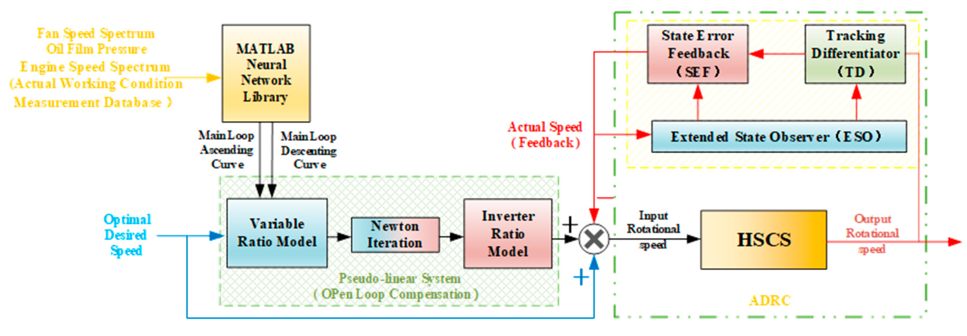
2. Overall Control Strategy Flow Chart of HSCS

The overall control strategy block diagram of HSCS is shown in Figure 1, which includes three modules: load condition identification, temperature closed loop control, and rotational speed closed loop control.

In Figure 1, the role of load condition identification is to determine whether the current hydro-viscous load is in an overloaded state. Hydro-viscous detachment control is performed if the load is too large in an overloaded state. The HSCS is performed if the load is judged to be a steady-state load.

The temperature closed loop control of HSCS takes the actual rotational speed, desired temperature, and actual temperature of the engine as input. Firstly, the oil temperature and water temperature are integrated, and the oil temperature and water temperature are converted into a single index. Combined with the actual rotational speed of the engine and fan, the optimal fan rotational speed control is calculated by MPC. Its function is to adjust input rotational speed according to the oil temperature and water temperature of the control transmission system.

The rotational speed closed loop control of HSCS is in the innermost layer of the whole control framework. The key to the rotational speed control is to overcome the serious nonlinearity of HSCS, such as large hysteresis, large dead zone, and parameter time-varying, and to improve the stability and robustness as much as possible on the premise of ensuring the control performance. Therefore, combining the inverter ratio model with the theory of ADRC, a rotational speed closed loop controller based on adaptive control parameter adjustment is designed. The inverter ratio means that after the desired rotational speed is input, the nominal input of the system is obtained through the nominal model, and then the actual output value of the system is calculated by the reverse ratio. The output value calculated by the inverter ratio is used as the feedforward input of the system.

In addition to the three basic control modules, it is also necessary to establish a data model based on the characteristic data of HSCS at different input rotational speeds and different oil temperatures, which can be used as a control model in the subsequent strategy design of HSCS, and a reference model for the modeling and simulation process of HSCS.

3. Establishment of HSCS Data Model

According to the characteristic data of steady-state HSCS with different input rotational speeds and different oil temperatures, a data-driven model describing the input/output rotational speed, control oil pressure, and lubricating oil temperature can be established. This model can be used not only as a control model in the design of subsequent strategies of HSCS but also as a reference model in the modeling and simulation process of HSCS.

However, HSCS has complex hysteresis characteristics, which are manifested as a multibranch nonlinearity in the relationship between input and output. As shown in Figure 2, the closed trajectory is formed by the reciprocating change in input in the input–output diagram. Among them, the main loop is the maximum hysteresis loop formed by the change between the maximum value u_max and the minimum value u_min of the input; the secondary loop is a hysteresis loop formed by the change between the local maximum and the local minimum. Therefore, in the establishment of the HSCS data model, the main loop data are used to establish an accurate model, and then the secondary loop data are mapped to the main loop.

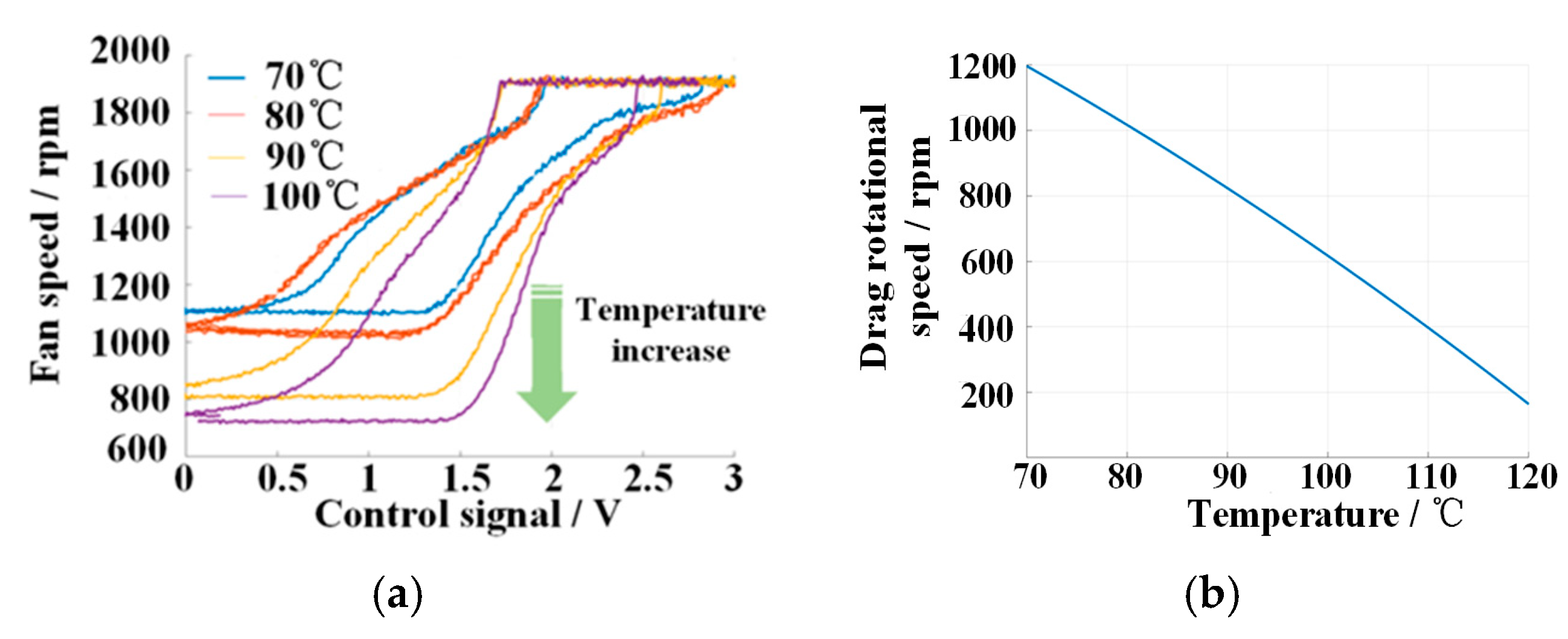
3.1. Hydro-Viscous Speed Disturbance Factor Analysis

The main factors affecting the output speed stability of a hydro-viscous drive system are engine rotational speed fluctuation, lubricating oil temperature change, and load change.

The statistical analysis of multiple sets of real vehicle road spectrum data is carried out to obtain the dynamic change law of engine rotational speed under typical working conditions, which is divided into steady state and dynamic state. The input and output rotational speed running-in curves are shown in Figure 3.

In Figure 3, the abscissa time is 8000 s. After a comprehensive analysis of the two figures, it can be concluded that the change rule of the engine is basically similar. As shown in Figure 3a, the representative of the five sections is selected, covering the engine rotational speed amplitude and frequency changes; it is enlarged to draw. In Figure 3b, it takes 6 s for the engine to go from the speed of 2400 rpm to the maximum speed of 1060 rpm, with a speed change of about 1340 rpm. In Figure 3c, it is concluded that the engine takes 4 s from 746 rpm to 1300 rpm, and the speed changes at about 554 rpm. Engine rotational speed went from 1100 rpm to 840 rpm in 2 s, a speed change of about 260 rpm. From Figure 3d, it is concluded that the engine changes from 1600 rpm to 700 rpm in 5 s, and the speed changes to about 900 rpm. Engine rotational speed changes from 1250 rpm to 900 rpm in 1 s, a speed change of about 350 rpm. Engine rotational speed changes from 839 rpm to 759 rpm in 2 s, a speed change of about 80 rpm. From Figure 3e, the engine changes from 2436 rpm to 1315 rpm in 8 s, and the speed changes about 1121 rpm. Engine rotational speed changes from 2424 rpm to 1723 rpm in 7 s, a speed change of about 700 rpm. From Figure 3f, it is concluded that the engine takes 3 s from 0 rpm to 950 rpm, and the speed changes about 950 rpm. Engine rotational speed changes from 1937 rpm to 0 rpm, which takes 16 s, with a speed change of about 1900 rpm.

At this point, the steady-state analysis is shown in Figure 4.

The spectrum analysis of engine and fan rotational speed shows that the fluctuation frequency band of engine rotational speed is about 1.2 Hz, and the fluctuation range is about 150 rpm.

The dynamic condition of engine input rotational speed is analyzed and is shown in Figure 5.

The spectrum characteristics are analyzed according to the curve. The spectrum analysis of the engine and fan rotational speed in the whole domain shows that the dynamic change rate(acceleration) of the engine rotational speed is concentrated at 0200 rpm/s.

The following is an analysis of the changes in lubricating oil temperature on the performance of HSCS disturbance. The change in lubricating oil temperature causes a change in oil viscosity, which mainly affects the strip phenomenon of HSCS. Let the lubricating oil temperature increase from 70 °C to 100 °C; the steady-state curves of HSC at different oil temperatures are obtained, as shown in Figure 6.

As the oil temperature ascends, the shape of the curve does not change significantly, but the drag rotational speed is significantly reduced. This happens due to the decrease in oil viscosity, leading to a reduction in drag torque.

Through the above analysis, the following conclusions can be obtained:

Lubricating oil temperature affects the discharge phenomenon; oil temperature increases with drag rotational speed, and torque decreases. The rate of change is −10 rpm/°C. The lubricating oil temperature will locally change the range of oil pressure, and the working point of the oil temperature ascending will move down. The lubricating oil temperature has little effect on the shape of the speed control characteristic curve and the closed loop control effect.

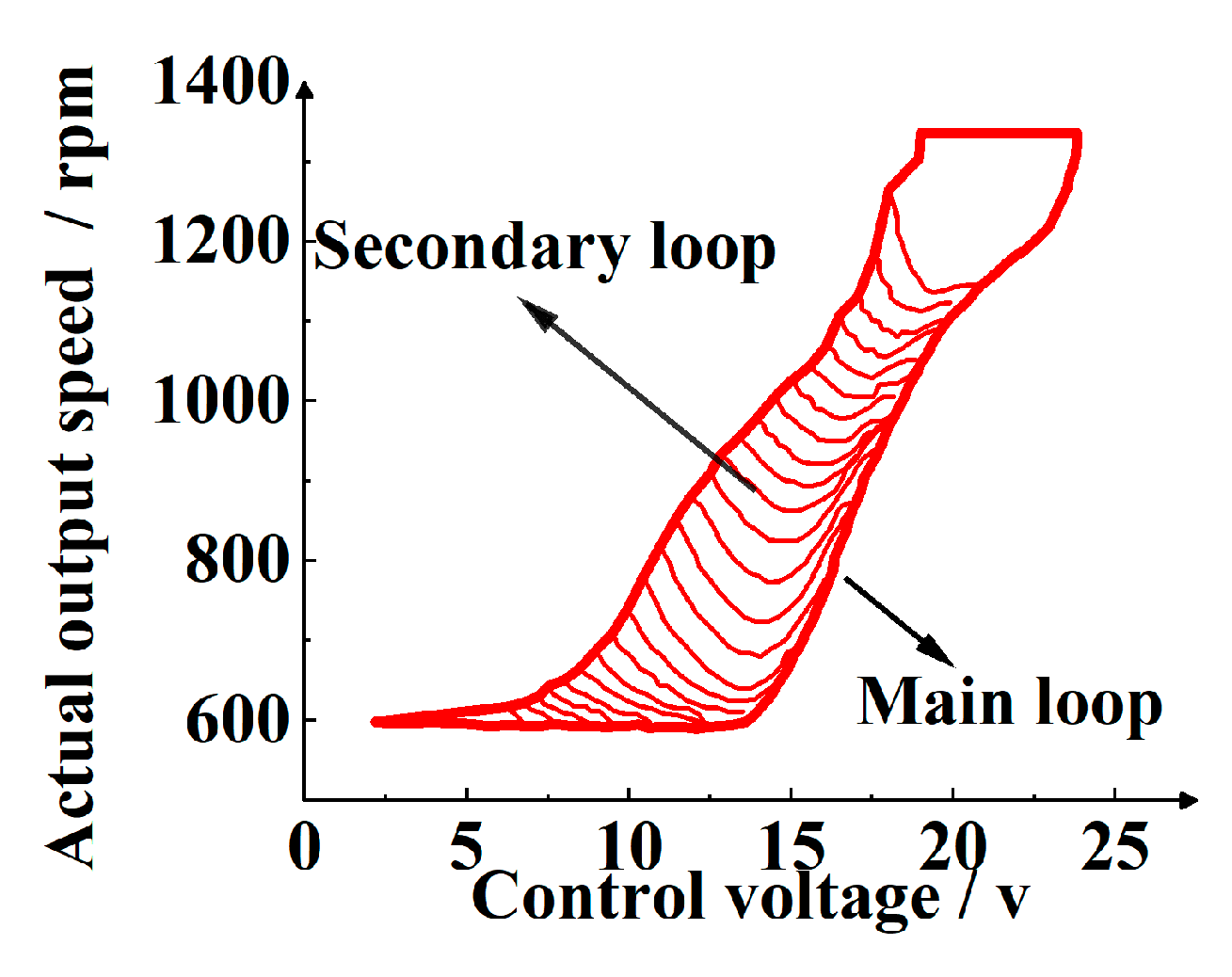
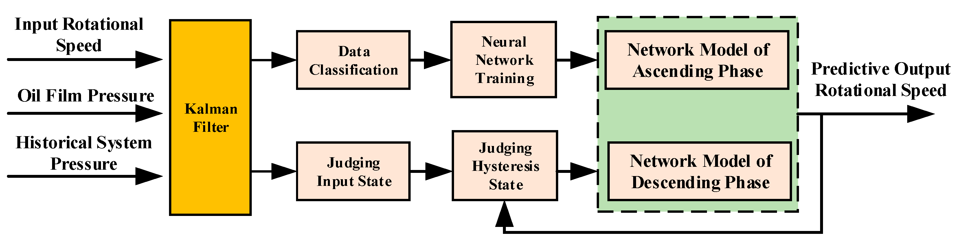
3.2. Main Loop Model Structure

When the inverter ratio model control is adopted, the accurate main loop model plays an important role in the regulation speed control of the inverter ratio model. However, the mechanism model and identification parameters of HSCS cannot be significantly deviated from the actual input and output main loop model. Therefore, the data classification and training of the neural network model through the bench data can realize the high-precision modeling of the input and output of the main loop.

Data-driven modeling regards the hydro-viscous clutch as a black box, does not analyze its internal mechanism, and uses the data of the input pressure or control quantity as well as the output rotational speed of the bench to directly model the on-line correction ability of the model is strong, which can be applied to highly nonlinear and severely uncertain systems. The data-driven modeling process mainly includes the data modeling process and model verification of the hydro-viscous clutch.

The modeling process is as follows in Figure 7.

In Figure 7, the input parameters are input rotational speed, historical control pressure, and oil film pressure, and the output parameters are predictive output rotational speed. The specific modeling process is summarized as follows:

(1)

Data filter: The Kalman filter algorithm is used to eliminate the abnormal disturbance of input control pressure and maintain the stable output of the model.

(2)

Data classification: The simulating data are divided into ascending and descending phases of pressure to distinguish control intervals.

(3)

Establish a neural network model: A back propagation neural network is selected, appropriate parameters are set to train the model in the ascending and descending phases, and model training and model verification are performed.

The final training results are shown in Figure 8.

In Figure 8, the maximum error of the model is 160 r/min, the average error is 15 r/min, the error percentage is 9.8%, and the model can represent the hysteresis characteristics of the system. The data-driven model of the Kalman filter, data classification, and neural network can describe the nonlinear characteristics of hydro-viscous clutch well and avoid parameter uncertainty in the process of mechanism modeling.

3.3. Prediction Secondary Loop Model

The law between the main loop and the secondary loop is found by using the variable ratio model, and the input and output curves of the pressure–speed main loop and the secondary loop of the hydro-viscous clutch are drawn. There are two steps: the linearization of the main loop model and the MPC of the secondary loop.

When the shape of the main hysteresis loop and the secondary hysteresis loop is similar, it can be approximately assumed that the main hysteresis loop and the secondary hysteresis loop can be linearly mapped to the same line. The schematic diagram is shown in Figure 9.

In Figure 9, assuming that the ascending and descending curves are replaced by two nonlinear functions f_up(p) and f_down(p), respectively. The ascend or descend of the inverse hysteresis model reference function f_r(p) is associated with the rotational speed ω. The linear formula in Figure 9 can be expressed as the following:

$$\begin{array}{ll}{g}_{l\to r}(p)& =g(p,p_l,{\omega }_l,p_r,{\omega }_r)\\ & ={\omega }_l+\frac{({\omega }_r-{\omega }_l)}{\left[f_r(p_r)-f_r(p_l)\right]}\left[f_r(p)-f_r(p_l)\right]\end{array}$$

(1)

If the input signal increases until the maximum threshold point, the trajectory starts from the lower point (p_l, ω_l) and approaches the higher threshold point (p_r, ω_r). The left turning point is defined as (p_left, ω_left), the right turning point is defined as (p_right, ω_right), and the desired speed on the secondary loop is ω_desired, which is mapped to the main loop. The calculation method is as follows:

$$f_r(p)=\frac{\left({\omega }_{\mathrm{desired}}-{\omega }_{\mathrm{left}}\right)\times \left[f_r\left(p_{\mathrm{right}}\right)-f_r\left(p_{\mathrm{left}}\right)\right]}{{\omega }_{\mathrm{right}}-{\omega }_{\mathrm{left}}}+f_r\left(p_{\mathrm{left}}\right)$$

(2)

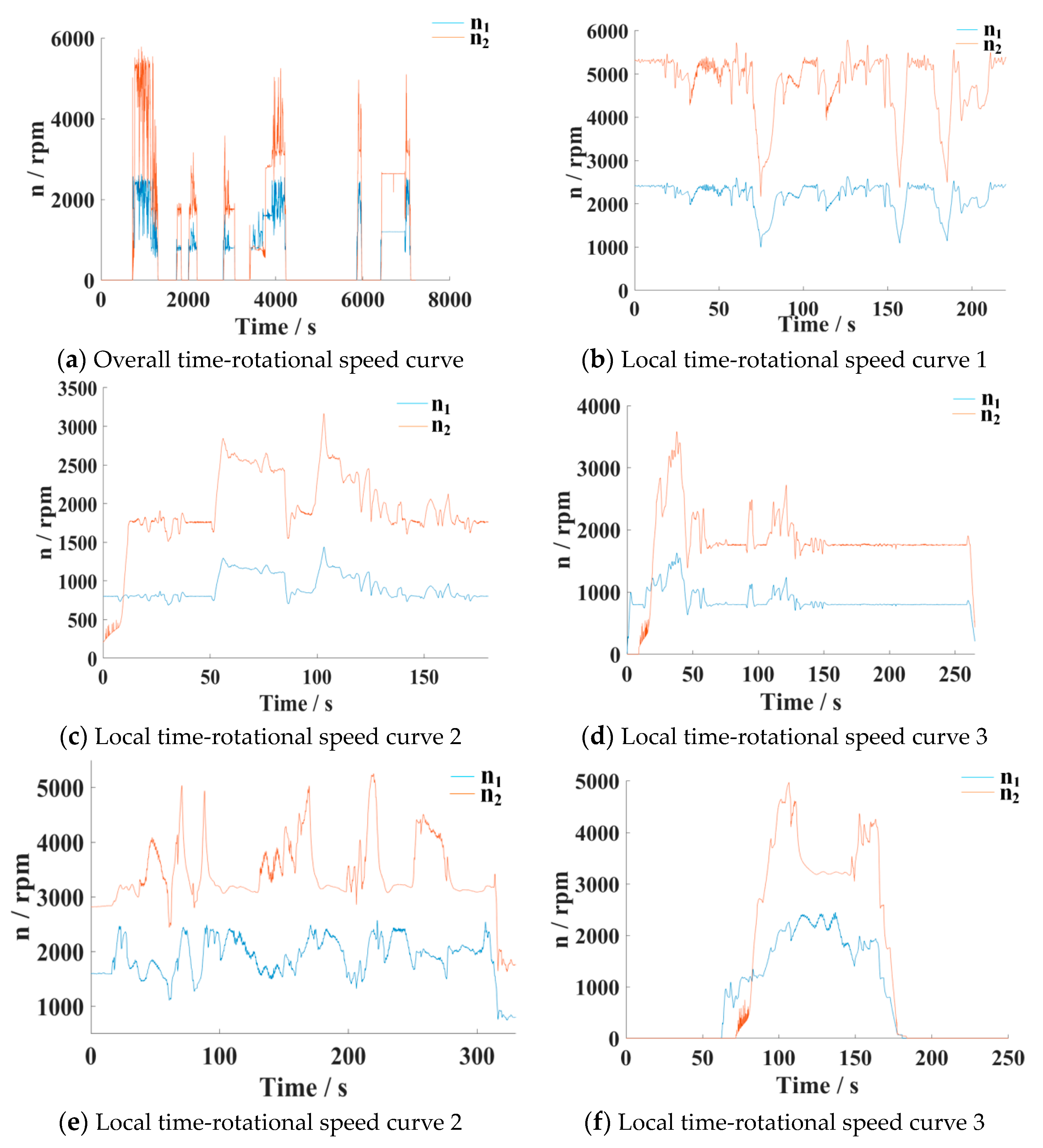
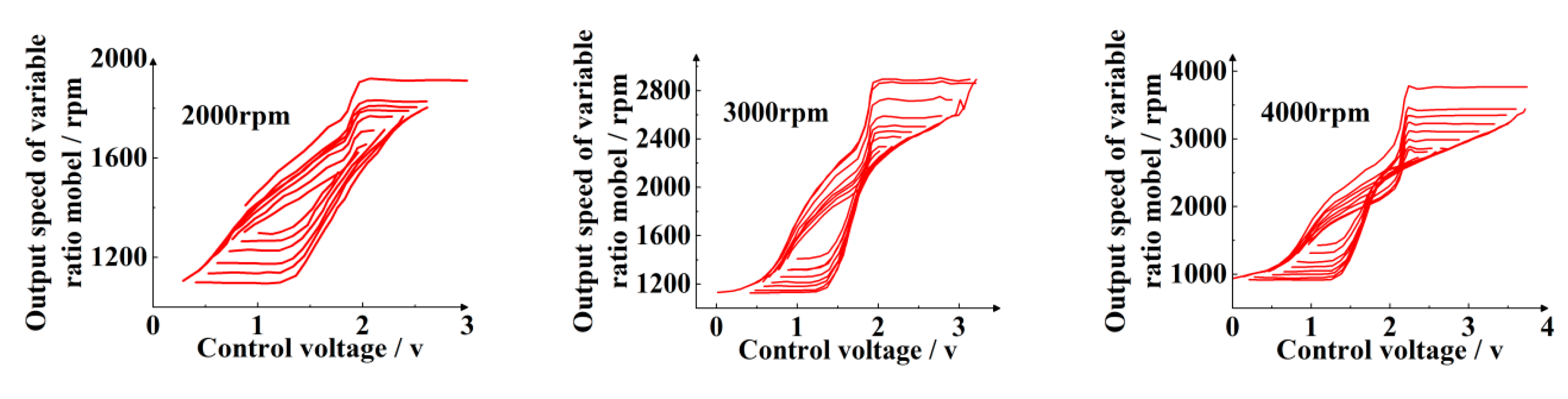
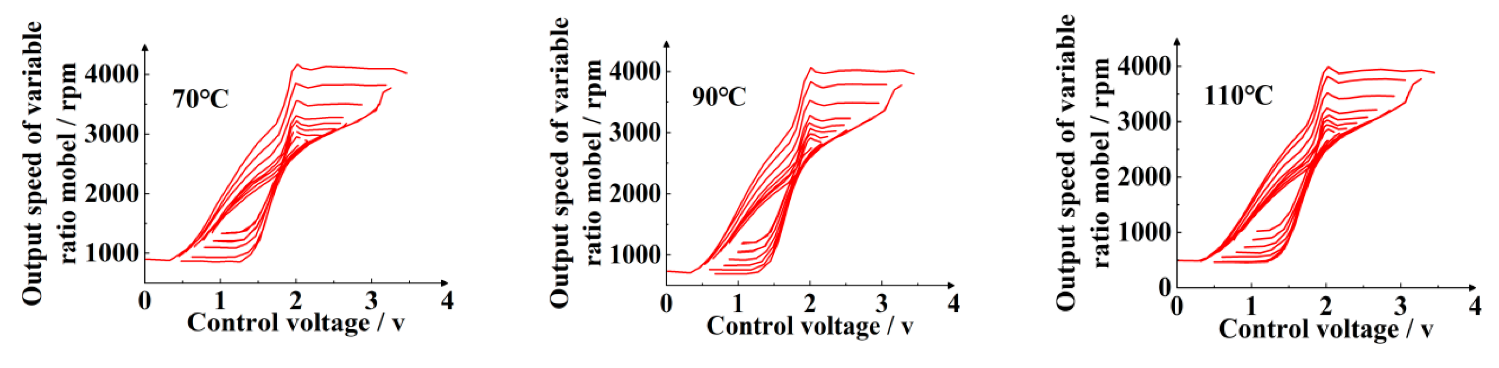
3.4. Generalization Capability Verification of Data Model

The data-driven model established in this project is used to verify the main loop and secondary loop laws of steady-state characteristics of HSCS under different input rotational speeds and different lubricating oil temperatures.

In Figure 10, the steady-state speed control characteristic curve is generated by the data-driven model at the lubricating oil temperature of 90 °C and different input rotational speeds.

In Figure 11, the steady-state speed control characteristic curve is generated by the data-driven model at the input rotational speed of 4000 rpm and different lubricating oil temperatures.

Through two diagrams, it can be proved that the steady-state speed control characteristic curves can be generated by the data-driven model under different lubricating oil temperatures and input rotational speeds, and the change rules of the main loop and the secondary loop can be characterized. Comparing the data-driven model with the simulating data, the main loop error is less than 10%, and the secondary loop is less than 20%, which has good generalization ability. The established model can be used as a control model in the design of subsequent strategies of HSCS.

4. Double Closed Loop Control of Temperature and Rotational Speed for HSCS

According to Section 2, Figure 1, the overall control strategy of HSCS is shown. In Section 4.1, the temperature closed loop control in the overall control strategy is first designed to obtain the optimal input rotational speed. Then, the speed closed loop control is designed according to the formed data model of HSCS and the desired rotational speed obtained in the temperature closed loop control in Section 4.2.

4.1. Closed Loop Control Method of Temperature

4.1.1. Basic Principle of Control

The working principle of temperature control based on MPC is shown in Figure 12 below.

In Figure 12, a closed loop controller of temperature is designed based on the principle of MPC. Its function is to output the optimal rotational speed control signal as the control input of the next rotational speed closed loop.

The closed loop controller of temperature consists of five parts: integrated treatment of the temperature of oil and water, temperature control model, constraint conditions, optimization objectives, and MPC.

Integrated treatment of temperature of oil and water: To reduce the calculation dimension and save the calculation power, the temperature of water and oil are calculated by integration (currently the mean value processing).

Temperature control model: The relationship model of engine rotational speed, fan rotational speed, and oil temperature and water temperature is obtained by system identification based on real vehicle data.

Constraint conditions: With the engine rotational speed as the constraint condition, the fan rotational speed cannot be higher than the current engine rotational speed multiplied by the transmission ratio k.

Optimization objectives: Oil temperature and water temperature control error and engine rotational speed fluctuations are the integrated optimization objectives.

MPC: Based on the temperature control model, optimization objectives and constraints, using quadratic optimization solver to calculate the optimal fan rotational speed control.

4.1.2. Integrated Treatment of Temperature of Oil and Water

There are two actual objectives of HSCS: water temperature and oil temperature, which have different desired values and working conditions. In order to reduce the control dimension and computational complexity, the oil–water temperature T_wo is used to identify the water temperature T_w and oil temperature T_o in this control method, which can be expressed as follows:

$$T_{wo}=k{T}_w+(1-k)T_o$$

(3)

where the water temperature and oil temperature adjustment coefficient k = 0.5.

The water temperature and oil temperature curves are shown in Figure 13.

In Figure 13, the oil temperature is higher than the water temperature, and it follows a nearly identical pattern of change. The middle line is the change curve of oil–water temperature, which is the average value of oil temperature and water temperature. Therefore, the above dimension reduction method is feasible.

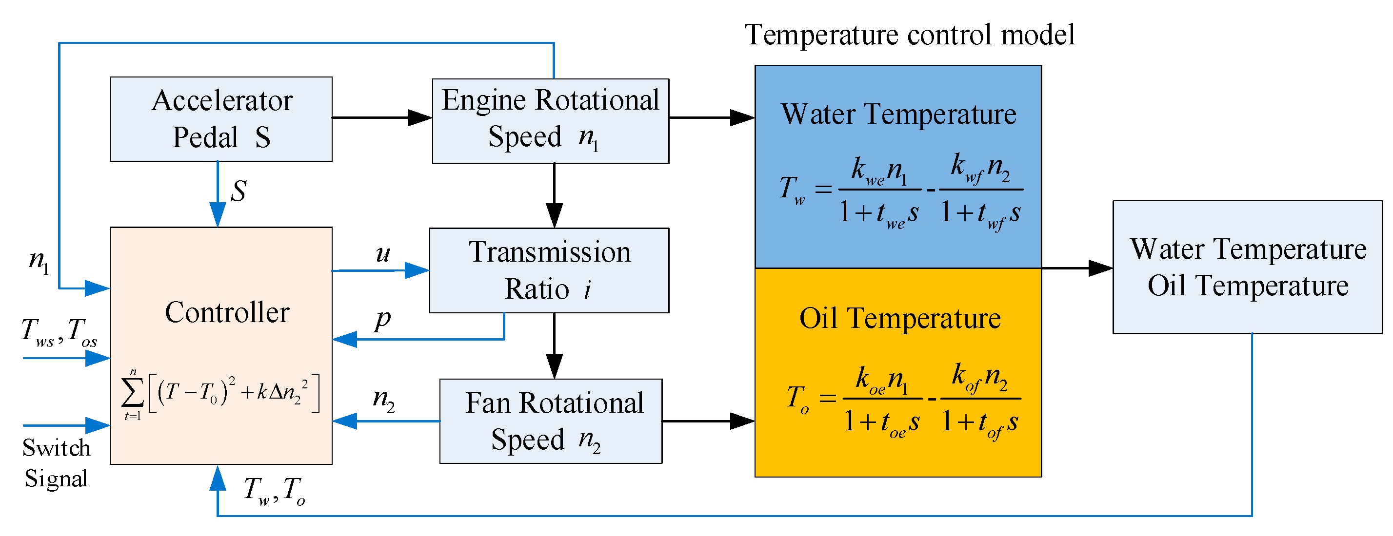
4.1.3. Temperature Control Model

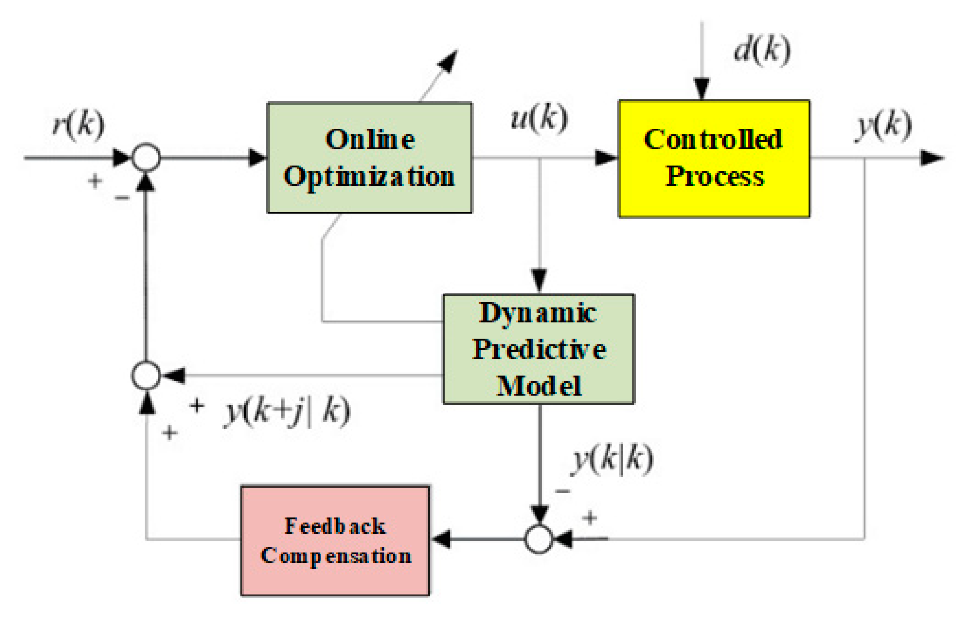
The temperature control model includes the following four models: Two temperature models include the engine-oil temperature model and the engine-water temperature model. The other two cooling models include the fan-oil temperature model and the fan-water temperature model. After the dimension reduction in oil temperature and water temperature, the temperature control models are simplified into two models: the engine-oil–water temperature model and the fan-oil–water temperature model. Both are described by inertial link, and the time constant of the proportional coefficient needs to be determined.

$$\begin{array}{l}{T}_w=f_{we}\left(n_1\right)-f_{wf}\left(n_2\right)\\ f_{we}\left(n_1\right)=\frac{k_{we}}{1+t_{we}s},f_{wf}\left(n_2\right)=\frac{k_{wf}}{1+t_{wf}s}\end{array}$$

(4)

where T_w denotes the oil–water temperature of the system; k_we denotes the engine -oil–water temperature amplification factor; k_wf denotes the fan-oil–water temperature amplification factor; t_we denotes the engine-oil–water temperature time constant; and t_wf denotes the fan-oil–water temperature time constant.

The above equation is a simplified temperature control model, which can be used as the input model of MPC.

Considering the control error of oil temperature and water temperature and the variable of fan rotational speed, the control error and the change in rotational speed are required to be small. The quadratic optimization objective function is as follows:

$$f\left(n_2\right)={\displaystyle \sum _{t=1}^n\left[{\left(\frac{\Delta T_w}{T_w}\right)}^2+{\left(\frac{\Delta T_o}{T_o}\right)}^2+k{\left(\frac{\Delta n_2}{n_2}\right)}^2\right]}$$

(5)

where ΔT_w/T_w denotes the water temperature control error; ΔT_o/T_o denotes the oil temperature control error; Δn₂/n₂ denotes the fan rotational speed variable; and k denotes the rotational speed influence weight.

The quadratic optimization objective function after dimension reduction is as follows:

$$f\left(n_2\right)={\displaystyle \sum _{t=1}^n\left[{\left(\frac{\Delta T_{wo}}{T_{wo}}\right)}^2+k{\left(\frac{\Delta n_2}{n_2}\right)}^2\right]}$$

(6)

where ΔT_wo/T_wo denotes the oil–water temperature control error; Δn₂/n₂ denotes the fan rotational speed variable; and k denotes the rotational speed influence weight.

By adjusting k to adjust the weight of the rotational speed change, the weight cannot be too large, which will affect the stability of the system and lead to the failure of temperature control.

Since the fan is directly driven by the engine, its maximum rotational speed is determined by the engine’s rotational speed. Therefore, the main constraint is designed as the engine rotational speed; that is, the fan rotational speed cannot be higher than the current engine rotational speed multiplied by the transmission ratio.

4.1.4. MPC

The MPC uses an existing model, the system’s current state, and the future control quantity to predict the system’s future output. Its basic principle and implementation process are shown in Figure 14.

In Figure 14, the time series length of the MPC output is an integer multiple of the control period. Since the future control quantity is unknown, it needs to be solved according to certain conditions to obtain the future control quantity sequence. After each control period, the system repredicts the future output of the system according to the current actual state. Therefore, MPC has three key steps: predictive model, rolling optimization, and feedback compensation.

Dynamic predictive model: The predictive model is the basis of control. Its role is to predict the future output of the system based on the historical information and future input of the object. The predictive models include state space equation, transfer function, step response, impulse response, neural network model, and so on.

Online optimization control: MPC determines the control sequence by controlling the optimal performance of a certain performance index, but the optimization is not carried out offline at one time but online repeatedly.

Model output feedback compensation: To prevent the deviation of the control from the ideal state caused by model mismatch or disturbance, at the novel sampling time, the actual output of the object is first detected, and this real-time information is used to correct the model-based predictive results. Then, a novel optimization is performed.

The state space equation of the temperature control model is as follows:

$$\begin{array}{l}\dot{\mathit{x}}=\mathit{Ax}+\mathit{Bu}+{\mathit{D}}_{\mathit{dis}}\\ \mathit{y}=\mathit{Cx}+\mathit{Du}\end{array}$$

(7)

where x denotes the state vector, y denotes the output, and u denotes the input.

The continuous state space equation needs to be discretized. The commonly used discretization methods include Euler formula discretization, backward difference, and bilinear transformation discretization. The discrete state space equation is as follows:

$$\begin{array}{l}{\mathit{x}}_{\mathit{k}+1} ={\mathit{A}}_{\mathit{d}} {\mathit{x}}_{\mathit{k}} +{\mathit{B}}_{\mathit{d}} {\mathit{u}}_{\mathit{k} }+{\mathit{D}}_{\mathit{d},\mathit{dis}} \\ {\mathit{y}}_{\mathit{k}} ={\mathit{C}}_{\mathit{d}} {\mathit{x}}_{\mathit{k}} +{\mathit{D}}_{\mathit{d}} {\mathit{u}}_{\mathit{k}} \end{array}$$

(8)

The predictive model is then derived as follows:

$$\left\{\begin{array}{ll}{\mathit{x}}_{\mathit{k}+\mathbf{1}}& ={\mathit{A}}_{\mathit{d}}{\mathit{x}}_{\mathit{k}}+{\mathit{B}}_{\mathit{d}}{\mathit{u}}_{\mathit{k}}+{\mathit{D}}_{\mathit{d},\mathit{dis}}\\ {\mathit{x}}_{\mathit{k}+\mathbf{2}}& ={\mathit{A}}_{\mathit{d}}{\mathit{x}}_{\mathit{k}+\mathbf{1}}+{\mathit{B}}_{\mathit{d}}{\mathit{u}}_{\mathit{k}+\mathbf{1}}+{\mathit{D}}_{\mathit{d},\mathit{dis}}\\ & ={\mathit{A}}_{\mathit{d}}\left({\mathit{A}}_{\mathit{d}}{\mathit{x}}_{\mathit{k}}+{\mathit{B}}_{\mathit{d}}{\mathit{u}}_{\mathit{k}}+{\mathit{D}}_{\mathit{d},\mathit{dis}}\right)+{\mathit{B}}_{\mathit{d}}{\mathit{u}}_{\mathit{k}+\mathbf{1}}+{\mathit{D}}_{\mathit{d},\mathit{dis}}\\ & ={\mathit{A}}_{\mathit{d}}^{\mathbf{2}}{\mathit{x}}_{\mathit{k}}+\left({\mathit{A}}_{\mathit{d}}{\mathit{B}}_{\mathit{d}}{\mathit{u}}_{\mathit{k}}+{\mathit{B}}_{\mathit{d}}{\mathit{u}}_{\mathit{k}+\mathbf{1}}\right)+{\mathit{A}}_{\mathit{d}}{\mathit{D}}_{\mathit{d},\mathit{dis}}+{\mathit{D}}_{\mathit{d},\mathit{dis}}\\ {\mathit{x}}_{\mathit{k}+\mathbf{3}}& ={\mathit{A}}_{\mathit{d}}{\mathit{x}}_{\mathit{k}+\mathbf{2}}+{\mathit{B}}_{\mathit{d}}{\mathit{u}}_{\mathit{k}+\mathbf{2}}+{\mathsf{\nu }}_{\mathit{d},\mathit{dis}}\\ & ={\mathit{A}}_{\mathit{d}}^{\mathbf{2}}{\mathit{x}}_{\mathit{k}+\mathbf{1}}+\left({\mathit{A}}_{\mathit{d}}{\mathit{B}}_{\mathit{d}}{\mathit{u}}_{\mathit{k}+\mathbf{1}}+{\mathit{B}}_{\mathit{d}}{\mathit{u}}_{\mathit{k}+\mathbf{2}}\right)+{\mathit{A}}_{\mathit{d}}{\mathit{D}}_{\mathit{d},\mathit{dis}}+{\mathit{D}}_{\mathit{d},\mathit{dis}}\\ {\mathit{x}}_{\mathit{k}+\mathbf{1}}& ={\mathit{A}}_{\mathit{d}}{\mathit{x}}_{\mathit{k}}+{\mathit{B}}_{\mathit{d}}{\mathit{u}}_{\mathit{k}}+{\mathit{D}}_{\mathit{d},\mathit{dis}}\\ & ={\mathit{A}}_{\mathit{d}}^{\mathbf{2}}{\mathit{x}}_{\mathit{k}+\mathbf{1}}+\left({\mathit{A}}_{\mathit{d}}{\mathit{B}}_{\mathit{d}}{\mathit{u}}_{\mathit{k}+\mathbf{1}}+{\mathit{B}}_{\mathit{d}}{\mathit{u}}_{\mathit{k}+\mathbf{2}}\right)+{\mathit{A}}_{\mathit{d}}{\mathit{D}}_{\mathit{d},\mathit{dis}}+{\mathit{D}}_{\mathit{d},\mathit{dis}}\\ & ={\mathit{A}}_{\mathit{d}}^{\mathbf{3}}{\mathit{x}}_{\mathit{k}}+\left({\mathit{A}}_{\mathit{d}}^{\mathbf{2}}{\mathit{B}}_{\mathit{d}}{\mathit{u}}_{\mathit{k}}+{\mathit{A}}_{\mathit{d}}{\mathit{B}}_{\mathit{d}}{\mathit{u}}_{\mathit{k}+\mathbf{1}}+{\mathit{B}}_{\mathit{d}}{\mathit{u}}_{\mathit{k}+\mathbf{2}}\right)+{\mathit{A}}_{\mathit{d}}^{\mathbf{2}}{\mathit{D}}_{\mathit{d},\mathit{dis}}+{\mathit{A}}_{\mathit{d}}{\mathit{D}}_{\mathit{d},\mathit{dis}}+{\mathit{D}}_{\mathit{d}}\\ & ⋮\\ {\mathit{x}}_{\mathit{k}+{\mathit{N}}_{\mathit{p}}}& ={\mathit{A}}_{\mathit{d}}^{{\mathit{N}}_{\mathit{p}}}{\mathit{x}}_{\mathit{k}}+\left({\mathit{A}}_{\mathit{d}}^{{\mathit{N}}_{\mathit{p}}-\mathbf{1}}{\mathit{B}}_{\mathit{d}}{\mathit{u}}_{\mathit{k}}+\mathit{L}+{\mathit{A}}_{\mathit{d}}^{{\mathit{N}}_{\mathit{p}}-{\mathit{N}}_{\mathit{c}}+\mathbf{1}}{\mathit{B}}_{\mathit{d}}{\mathit{u}}_{\mathit{k}+\mathbf{1}}+{\mathit{A}}_{\mathit{d}}^{{\mathit{N}}_{\mathit{p}}-{\mathit{N}}_{\mathit{c}}}{\mathit{B}}_{\mathit{d}}{\mathit{u}}_{\mathit{k}+{\mathit{N}}_{\mathit{c}}-\mathbf{1}}\right)\\ & +\left({\mathit{A}}_{\mathit{d}}^{{\mathit{N}}_{\mathit{p}}-\mathbf{1}}{\mathit{D}}_{\mathit{d},\mathit{dis}}+\mathit{L}+{\mathit{A}}_{\mathit{d}}{\mathit{D}}_{\mathit{d},\mathit{dis}}+{\mathit{D}}_{\mathit{d},\mathit{dis}}\right)\end{array}\right.$$

(9)

Collate to obtain

$$\mathit{X}=\mathit{F}{\mathit{X}}_{\mathbf{0}}+\mathit{\Phi }\mathit{U}+\mathit{E}$$

(10)

where

$$\left\{\begin{array}{l}\mathit{X}={\left[{\mathit{x}}_{\mathit{k}+\mathbf{1}},{\mathit{x}}_{\mathit{k}+\mathbf{2}},\mathit{L},{\mathit{x}}_{\mathit{k}+{\mathit{N}}_{\mathit{P}}}\right]}^{\mathit{T}}\\ {\mathit{X}}_{\mathbf{0}}={\mathit{x}}_{\mathit{k}};\\ \mathit{U}={\left[{\mathit{u}}_{\mathit{k}},{\mathit{u}}_{\mathit{k}+\mathbf{2}},\mathit{L},{\mathit{u}}_{\mathit{k}+{\mathit{N}}_{\mathit{c}}-\mathbf{1}}\right]}^{\mathit{T}}\\ \mathit{F}={\left[{\mathit{A}}_{\mathit{d}},{\mathit{A}}_{\mathit{d}}^{\mathbf{2}},\mathit{L},{\mathit{A}}_{\mathit{d}}^{{\mathit{N}}_{\mathit{p}}}\right]}^{\mathit{T}}\\ \mathit{\Phi }=\left[\begin{array}{cccc}{\mathit{B}}_{\mathit{d}}& \mathbf{0}& \mathit{L}& \mathbf{0}\\ {\mathit{A}}_{\mathit{d}}{\mathit{B}}_{\mathit{d}}& {\mathit{B}}_{\mathit{d}}& \mathit{L}& \mathbf{0}\\ \mathit{M}& \mathit{M}& \mathit{O}& \mathit{M}\\ {\mathit{A}}^{{\mathit{N}}_{\mathit{p}}-\mathbf{1}}\mathit{d}{\mathit{B}}_{\mathit{d}}& {\mathit{A}}^{{\mathit{N}}_{\mathit{p}}-\mathbf{2}}\mathit{d}{\mathit{B}}_{\mathit{d}}& \mathit{L}& {\mathit{A}}_{\mathit{d}}^{{\mathit{N}}_{\mathit{p}}-{\mathit{N}}_{\mathit{c}}}{\mathit{B}}_{\mathit{d}}\end{array}\right]\\ \mathit{E}={\left[{\mathit{D}}_{\mathit{d},\mathit{dis}},{\mathit{A}}_{\mathit{d}}{\mathit{D}}_{\mathit{d},\mathit{dis}}+{\mathit{D}}_{\mathit{d},\mathit{dis}},\mathit{L},\underset{\mathit{i}=\mathbf{0}}{\overset{{\mathit{N}}_{\mathit{p}}-\mathbf{1}}{\mathsf{å}}}{\mathit{A}}_{\mathit{k}}^{\mathit{i}}{\mathit{D}}_{\mathit{d},\mathit{dis}}\right]}^{\mathit{T}}\end{array}\right.$$

(11)

where X denotes state vector, X₀ denotes initial condition, U denotes input matrix, and E denotes constant.

The minimum error between the desired output and the predictive output of the system is taken as the cost function.

$$\begin{array}{ll}\mathit{J}& ={\left(\mathit{Y}-{\mathit{Y}}_{\mathit{ref}}\right)}^{\mathit{T}}{\mathit{Q}}_{\mathit{e}}\left(\mathit{Y}-{\mathit{Y}}_{\mathit{ref}}\right)+{\mathit{U}}^{\mathit{T}}{\mathit{R}}_{\mathit{e}}\mathit{U}\\ & ={\left({\mathit{F}}_{\mathit{y}}{\mathit{X}}_{\mathbf{0}}+{\mathit{\Phi }}_{\mathit{y}}\mathit{U}+{\mathit{E}}_{\mathit{y}}-{\mathit{Y}}_{\mathit{ref}}\right)}^{\mathit{T}}{\mathit{Q}}_{\mathit{e}}\left({\mathit{F}}_{\mathit{y}}{\mathit{X}}_{\mathbf{0}}+{\mathit{\Phi }}_{\mathit{y}}\mathit{U}+{\mathit{E}}_{\mathit{y}}-{\mathit{Y}}_{\mathit{ref}}\right)+{\mathit{U}}^{\mathit{T}}{\mathit{R}}_{\mathit{e}}\mathit{U}\\ & ={\mathit{U}}^{\mathit{T}}\left({\mathit{\Phi }}_{\mathit{y}}^{\mathit{T}}{\mathit{Q}}_{\mathit{e}}{\mathit{\Phi }}_{\mathit{y}}+{\mathit{R}}_{\mathit{e}}\right)\mathit{U}+{\mathit{U}}^{\mathit{T}}\left[\mathbf{2}{\mathit{\Phi }}_{\mathit{y}}^{\mathit{T}}{\mathit{Q}}_{\mathit{e}}\left({\mathit{F}}_{\mathit{y}}{\mathit{X}}_{\mathbf{0}}+{\mathit{E}}_{\mathit{y}}-{\mathit{Y}}_{\mathit{ref}}\right)\right]\\ & +{\left({\mathit{F}}_{\mathit{y}}{\mathit{X}}_{\mathbf{0}}+{\mathit{E}}_{\mathit{y}}-{\mathit{Y}}_{\mathit{ref}}\right)}^{\mathit{T}}{\mathit{Q}}_{\mathit{e}}\left({\mathit{F}}_{\mathit{y}}{\mathit{X}}_{\mathbf{0}}+{\mathit{E}}_{\mathit{y}}-{\mathit{Y}}_{\mathit{ref}}\right)\end{array}$$

(12)

The cost function can be abbreviated as follows:

$$\mathit{J}={\mathit{U}}^{\mathit{T}}\mathit{RU}+\mathbf{2}{\mathit{U}}^{\mathit{T}}\mathit{Q}+\mathit{P}$$

(13)

where Q denotes the state weight matrix, R denotes the control input weight matrix, and P denotes a constant. Obviously, the cost function is a QP problem.

Suppose that only the upper and lower bounds of control variables are considered; then the constraint of matrix U is as follows:

$$\left[\begin{array}{c}\mathit{I}\\ -\mathit{I}\end{array}\right]\mathit{U}\ge \left[\begin{array}{c}{\mathit{U}}_{min}\\ -{\mathit{U}}_{max}\end{array}\right]$$

(14)

It can be seen from the above that the solution of the MPC problem is finally transformed into the solution of the QP problem. For the QP problem, there are many methods and open-source libraries in engineering that can be solved. Common methods include the Karush Kuhn Tucker (KKT) multiplier method, gradient descent method, Newton method, particle swarm optimization algorithm/pigeon group optimization algorithm, and other heuristic algorithms [28,29,30,31].

The hydro-viscous speed control system realizes control over the oil temperature and water temperature within the transmission system; the temperature control principle is illustrated in Figure 15. The controller takes switch signals, oil temperature, water temperature, target temperature, engine rotational speed, and fan rotational speed as input signals and outputs oil pressure control signal. It regulates the transmission ratio of the hydro-viscous clutch to control the fan rotational speed, thereby regulating oil temperature and water temperature.

In this control process, the fan rotational speed is constrained by both the transmission system and the engine rotational speed, with the maximum speed not exceeding 2.5 times the engine rotational speed. The temperature control model comprises two components: an engine-related heating model and a fan rotational speed-related cooling model.

In addition, the hydro-viscous speed control system has two control objectives: water temperature and oil temperature, each with different target values and operating states. In the initial derivation process, to reduce control dimensions and computational complexity, this control method uses the oil–water temperature to represent both water temperature and oil temperature; however, there still exists a disparity in the variation patterns and actual numerical values between them.

Taking all these considerations into account, this paper uses the particle swarm algorithm to solve the QP problem [32]. The biggest advantage of this type of algorithm is that it does not need to have a precise portrayal of the system model, completely using a heuristic algorithm ‘trial and error‘ to find, and the amount of computation required is not large. Heuristic algorithms are doomed to have no rigorous proof in mathematics, but many of these algorithms have achieved good results in practice.

In the solving process, we expanded the state space model based on water temperature and oil temperature:

$$\begin{array}{l}T=T_w+T_o=[f_{we}\left(n_1\right)-f_{wf}\left(n_2\right)]+[f_{oe}\left(n_1\right)-f_{of}\left(n_2\right)]\\ f_{we}\left(n_1\right)=\frac{k_{we}}{1+t_{we}s},f_{wf}\left(n_2\right)=\frac{k_{wf}}{1+t_{wf}s}\\ f_{oe}\left(n_1\right)=\frac{k_{oe}}{1+t_{oe}s},f_{of}\left(n_2\right)=\frac{k_{of}}{1+t_{of}s}\end{array}$$

(15)

where T denotes the oil–water temperature of the system; k_we denotes the engine-water temperature amplification factor; k_wf denotes the fan-water temperature amplification factor; t_we denotes the engine-water temperature time constant; t_wf denotes the fan-water temperature time constant; k_oe denotes the engine-oil temperature amplification factor; k_of denotes the fan-oil temperature amplification factor; t_oe denotes the engine-oil temperature time constant; and t_of denotes the fan-oil temperature time constant.

To reduce the control errors of oil temperature, water temperature, and fan rotational speed variation, the quadratic optimization objective function is designed as follows:

$$f\left(n_2\right)={\displaystyle \sum _{t=1}^n\left[{\left(\frac{\Delta T_w}{T_w}\right)}^2+{\left(\frac{\Delta T_o}{T_o}\right)}^2+k{\left(\frac{\Delta n_2}{n_2}\right)}^2\right]}$$

(16)

The particle swarm is randomly initialized in each solution space, and the number of variables of the problem to be optimized determines the dimension of the solution space. It is based on the initial position and initial speed of each particle and then through iterative optimization. In each iteration, the optimal solution particle found by a single particle itself in the iteration process is called the individual extreme value. The optimal solution particle found by all particles in the iterative process is the global extreme value. Each particle updates its spatial position and flight speed in the solution space by tracking two ‘extreme value’: The overall operation logic is shown in Figure 16.

Finally, the temperature closed loop compensates for the temperature effect through MPC to obtain the optimal speed, which is input into the speed closedloop control. Then, the paper studies the closed loop control method of rotational speed.

To test the effectiveness of the particle swarm optimization algorithm in this approach, we conducted simulations and experiments on the multi-parameter hydro-viscous speed control system. The specific steps and results are as follows:

Testing steps and methods: The inlet oil temperature is set at 70 °C and 80 °C, and the input rotational speed of the hydro-viscous clutch is 4501 ± 50 r/min; the actual load of the fan is simulated to ensure that the load is 110 ± 20 Nm when the output rotational speed is 2500 ± 50 r/min, and the load is 380 ± 20 Nm when the output rotational speed is 4501 ± 50 r/min. Starting from zero pressure, gradually adjust the control pressure to rise to 0.2 ± 0.1 MPa, and test and record the output speed of the liquid viscosity. Starting from zero pressure again, gradually adjust the control pressure to rise to 0.4 ± 0.1 MPa, and test and record the output speed of the liquid viscosity.

Define the simulated value and experimental value of the output rotational speed as and, respectively. Under equivalent conditions (input rotational speed of 4501 r/min and oil pressure of 0.2 MPa and 0.4 MPa), conduct simulation and experimentation using the multi-parameter hydro-viscous speed control system to obtain the output rotational speed. Finally, calculate the error between the simulated value and the experimental value of the output rotational speed using the following formula:

$$\delta =\frac{\left|n_t-n_s\right|}{n_t}\times 100\%$$

(17)

If the error between the simulated value and experimental value of the output rotational speed does not exceed 20%, then the test is considered successful.

According to the above steps, experimental and simulated results under two scenarios with oil temperatures set at 70 °C and 80 °C, respectively, were selected for analysis to further verify the method proposed in this paper.

When the oil temperature is set to 70 °C, experiments and simulations were conducted separately, yielding the following results Figure 17 and Figure 18 and

Table 1. Comparison of experimental and simulated values of oil pressure and output rotational speed when oil temperature is 70 °C.

	Oil Pressure (MPa)	Experimental Value (r/min)	Simulated Value (r/min)	Error (%)
1	0.205	2039	2198	7.9
2	0.407	2964	2850	3.8

:

When temperature is set to 80 °C, experiments and simulations were conducted separately, yielding the following results Figure 19 and Figure 20 and

Table 2. Comparison of experimental and simulated values of oil pressure and output rotational speed when oil temperature is 80 °C.

	Oil Pressure (MPa)	Experimental Value (r/min)	Simulated Value (r/min)	Error (%)
1	0.206	1988	2148	8.0
2	0.402	2814	2850	1.3

:

Test Conclusion: After conducting experiments and simulations with oil temperatures set to 70 °C and 80 °C, it was found that the error between experimental values and simulated values did not exceed 8%. The test is considered successful.

4.2. Closed Loop Control Method of Rotational Speed

4.2.1. Basic Principle of Control

The closed loop control schematic of rotational speed for HSCS is shown in Figure 21.

The key to the rotational speed control closed loop is to overcome the serious nonlinearity such as large hysteresis, large dead zone, and parameter time-varying of the hydro-viscous clutch and to improve the stability and robustness as much as possible under the premise of ensuring the control performance. The traditional PID control cannot dynamically change the control parameters according to the changes in the model and working conditions. Therefore, combining the inverter ratio model with the idea of ADRC, an outer loop controller of rotational speed based on adaptive control parameter adjustment is designed. Aiming at the serious nonlinear problem of the hydro-viscous clutch, it is necessary to comprehensively consider various nonlinear control schemes, focusing on the hysteresis nonlinear problem. The control scheme adopted includes open loop control based on the inverse model and adaptive closedloop control based on the hysteresis model.

There are many nonlinear characteristics in the ascending and descending phases of HSCS, including a wide range of dead zones and saturated zones, accounting for two-thirds of the entire adjustable domain. In addition, there is about 40% hysteresis, which greatly increases the difficulty of control. To reduce the influence of this mixed nonlinearity, a control strategy combining feedforward control based on an inverter ratio model and adaptive closed loop control is proposed, and the corresponding ADRC method is developed. The inner loop control of the rotational speed adopts the inverse ratio model based on the neural network as the feedforward loop, and the closed loop control method based on the ADRC algorithm is used to form the feedback loop.

The main objective of open loop control based on the inverter ratio model is to determine the approximate range of the input control signal. The main idea is to compensate the original nonlinear large hysteresis system into a pseudo-linear system through the inverter ratio compensation control. This linear compensation process can effectively remove the saturation dead zone characteristics of the ascending and descending phases. The compensated pseudo-linear model is called the nominal model of the system, and the nominal model can be set artificially. After inputting the desired rotational speed, the nominal input of the system is obtained by the nominal model, and then the actual output value of the system is calculated by the inverter ratio. The inverter ratio calculation process can improve the hysteresis characteristics of the system, and the output value calculated by the inverter ratio is used as the feedforward input of the system.

The inverter ratio model is a difficult point in the control process, which is mainly composed of two parts. The first is to determine the data model of the main loop of the variable ratio model according to different engine rotational speeds and other conditions, and the second is the calculation process of the inverter ratio. The data model of the main loop is very important to the control process. Here, the neural network learning method is used to model the main loop. After obtaining the accurate main loop model, the inversion ratio model is mainly used to establish the mapping relationship between the main loop and the secondary loop of the system. The main advantage of the variable ratio model is that it follows the hysteresis characteristics: the consistency of the secondary loop and the memory erase characteristics. This strategy can provide the correct path for the mapping strategy.

After obtaining the feedforward compensation value output by the inverter ratio model, to further improve the accuracy of the hydro-viscous clutch speed control, it is necessary to find an ADRC method to design a closed loop control strategy for the above open loop pseudo-linear system to fine-tune the rotational speed control. First, an inverse hysteresis model of feedforward compensation needs to be established.

4.2.2. Inverter Ratio Model of Feedforward Compensation

The mapping information of the main loop was used to obtain the information of the secondary loop through the inverter ratio modeling, to obtain the feedforward compensation value of the clutch of HSCS, and to compensate the original nonlinear large hysteresis system into a pseudo-linear system through the inverter ratio compensation control.

According to the diagram of the main circuit, secondary circuit, and mapping method in Figure 5, when the shapes of the main hysteresis loop and secondary hysteresis loop are similar, it can be approximately assumed that the main hysteresis loop and secondary hysteresis loop can be linearly mapped to the same line. The ascending and descending curves are replaced by two nonlinear functions f_up(p) and f_down(p), respectively.

If the input signal increases until the maximum threshold point, the trajectory starts from the lower point (p_l, ω_l) and approaches the higher threshold point (p_r, ω_r). The left turning point is defined as (p_left, ω_left), the right turning point is defined as (p_right, ω_right), and the desired rotational speed on the secondary loop is ω_desired, which is mapped to the main loop accordingly. The update rules of the left turning point (p_left, ω_left) and the right turning point (p_left, ω_left) and the feedforward compensation value algorithm are as follows.

For any point (p_k, ω_k) satisfying p_m ≤ p_k ≤ p_r and ω_k = g_l→r (p_k), we can obtain the following:

$${\omega }_k=g_{l\to r}\left(p_k\right)$$

(18)

$${\omega }_m=g_{l\to r}\left(p_m\right)={\omega }_l+\frac{\left({\omega }_r-{\omega }_l\right)}{\left[f_r\left(p_r\right)-f_r\left(p_l\right)\right]}\left[f_r\left(p_m\right)-f_r\left(p_l\right)\right]$$

(19)

$${\omega }_k=g_{m\to r}\left(p_k\right)={\omega }_m+\frac{\left({\omega }_r-{\omega }_m\right)}{\left[f_r\left(p_r\right)-f_r\left(p_m\right)\right]}\left[f_r\left(p_k\right)-f_r\left(p_m\right)\right]$$

(20)

By Equation (20), there is

$$\begin{array}{l}\frac{\left({\omega }_r-{\omega }_m\right)}{\left[f_r\left(p_r\right)-f_r\left(p_m\right)\right]}\\ \begin{array}{l}=\frac{{\omega }_r-\left\{{\omega }_l+\frac{\left({\omega }_r-{\omega }_l\right)}{\left[f_r\left(p_r\right)-f_r\left(p_l\right)\right]}\left[f_r\left(p_r\right)-f_r\left(p_l\right)\right]\right\}}{\left[f_r\left(p_r\right)-f_r\left(p_m\right)\right]}\hfill \\ =\frac{\left({\omega }_r-{\omega }_l\right)\left\{1-\frac{\left[f_r\left(p_m\right)-f_r\left(p_l\right)\right]}{\left[f_r\left(p_r\right)-f_r\left(p_l\right)\right]}\right\}}{\left[f_r\left(p_r\right)-f_r\left(p_m\right)\right]}\hfill \\ =\frac{\left({\omega }_r-{\omega }_l\right)}{\left[f_r\left(p_r\right)-f_r\left(p_l\right)\right]}\hfill \end{array}\end{array}$$

(21)

Substituting Equations (19) and (21) into (20), there is

$$\begin{array}{ll}{\omega }_k& ={\omega }_l+\frac{\left({\omega }_r-{\omega }_l\right)}{\left[f_r\left(p_r\right)-f_r\left(p_l\right)\right]}+\frac{\left({\omega }_r-{\omega }_m\right)}{\left[f_r\left(p_r\right)-f_r\left(p_m\right)\right]}\left[f_r\left(p_k\right)-f_r\left(p_m\right)\right]\\ & =g_{l\to r}\left(p_k\right)\end{array}$$

(22)

where K_p denotes the proportional coefficient. To simplify the tuning process of K_p, β₁, and β₂, let K_p = ω_c, β₁ = 2ω₀, and β₂ = ω₀, where ω_c denotes the controller bandwidth, and ω₀ denotes the observer bandwidth.

The process of obtaining the compensation amount by the above nonlinear mapping can effectively remove the saturated dead zone characteristics of the ascending and descending phases. The compensated pseudo-linear model is called the nominal model of the system, and the nominal model can be set artificially. After inputting the desired rotational speed, the nominal input of the system is obtained by the nominal model, and then the actual output value of the system is calculated by the inverter ratio. The inverter ratio calculation process can improve the hysteresis characteristics of the system, and the output value calculated by the inverter ratio is used as the feedforward input of the system.

The difficulty of realizing this compensation controller is whether the inverter ratio model can be accurately constructed. The construction process of the inverter ratio model is mainly divided into two parts. One is to determine the data model of the main loop of the rotational speed control system according to different engine input rotational speeds and other conditions. The data model of the main loop is very important to the control process. Here, the neural network learning method is used to model the main loop. The second part is the inverter ratio calculation process. The inverter ratio calculation method can be used to map the relationship between the main loop and the secondary loop of the system. Through this process, the data model of the secondary loop is obtained. The main advantage of the inverter ratio calculation method is that it follows the characteristics of the hysteresis loop: secondary loop consistency and memory erase characteristics. This calculation method can accurately map the secondary loop information.

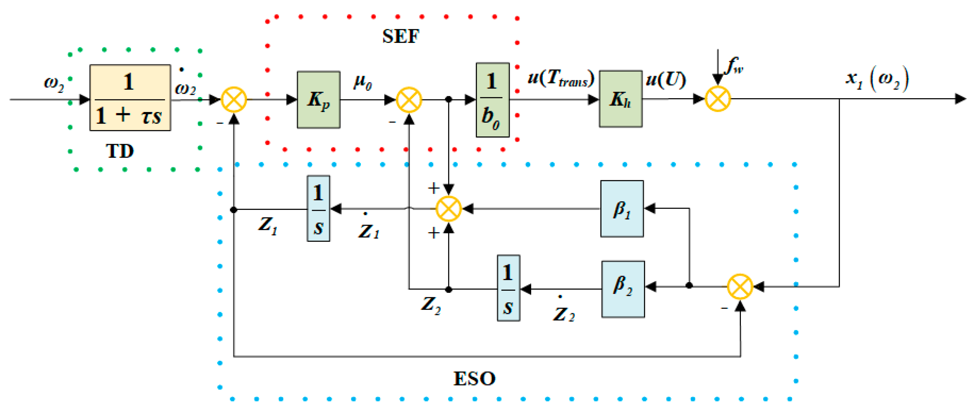
4.2.3. Feedback Control of ADRC

After obtaining the feedforward compensation value output by the inverse hysteresis model, to further improve the accuracy of the hydro-viscous clutch speed control, the method of ADRC is used as the closed loop control strategy of the above open loop pseudo-linear system to fine-tune the rotational speed control.

Two principles should be followed in the design of control law: Whether the prior model is needed and whether there is a large disturbance. Due to the complexity of the principle of the hydro-viscous clutch, the process of obtaining the mechanism model represented by the differential equation is complex, and the accuracy of the model cannot be guaranteed. Here, the controller that does not depend on the system model is selected, and the model is approximated as a linear system near the control point. Considering the low control resolution of the nonlinear section of the system, it is not appropriate to use linear control strategies such as PID with uncontrollable input. In addition, due to the large frequency, wide range, and large amplitude of the input rotational speed change, the controller needs to have a strong ability to disturbance rejection at the control point. In summary, to achieve precise speed control at the control point, the integrated control ideas of ADRC are used to adapt to this input controllable, state estimable fine-tuning control function in this simulation.

The ADRC consists of a tracking differentiator (TD), extended state observer (ESO), and state error feedback (SEF). According to the torque transfer formula of the hydro-viscous clutch, the first-order inertia link 1/(1 + τs) is used as the TD to suppress overshoot and arrange the transition process, where τ is the inertia time constant. Set ${\tilde{\omega }}_2$ to the tracking input of ${\omega }_2^{*}$, and then set ${\omega }_2^{*}/(1+\tau s)$. The state equation for rotational speed ω₂ is expressed as follows:

$${\dot{\omega }}_2=\frac{u}{J}-\frac{T_{fan}+T_f}{J} \mathrm{or} {\dot{\omega }}_2=b_{0}u+f_{\omega }$$

(23)

where f_w= −(T_fan + T_f)/J denotes the total disturbance, and b₀ denotes an adjustable coefficient. In the inverse hysteresis compensation model, u can be approximated as u = T_trans = K_hU.

Let x₁ = ω₂ and x₂ = f_w; the state equation of the friction pair pressure can be expressed as follows:

$$\left\{\begin{array}{l}\dot{\mathit{x}}=\mathit{Ax}+\mathit{Bu}+\mathit{Eh}\hfill \\ \mathit{y}=\mathit{Cx}\hfill \end{array}\right.$$

(24)

where $\mathit{A}=\left[\begin{array}{l}\mathbf{0} \mathbf{1}\\ \mathbf{0} \mathbf{0}\end{array}\right], \mathit{B}=\left[\begin{array}{l}{\mathit{b}}_{\mathbf{0}}\\ \mathbf{0}\end{array}\right], \mathit{C}=\left[\mathbf{1} \mathbf{0}\right], \mathit{E}=\left[\begin{array}{l}\mathbf{0}\\ \mathbf{1}\end{array}\right]$ denotes the system output.

The corresponding linear state observer is as follows:

$$\left\{\begin{array}{l}\dot{z}=\mathit{A}+\mathit{Bu}+\mathit{L}(\mathit{y}-\hat{\mathit{y}})\hfill \\ \hat{\mathit{y}}=\mathit{C}z\hfill \end{array}\right.$$

(25)

where z₁ and z₂ denote the estimates of x₁ and x₂, respectively. L = [β₁ β₂]. Let β₁ = 2ω₀ and β₂ = ω₀,

Where ω₀ denotes the observer bandwidth. Equation (25) can be extended to the following:

$$\left\{\begin{array}{l}{\dot{z}}_1=z_2-{\beta }_1\left(z_1-x_1\right)+b_{0}u\hfill \\ {\dot{z}}_2=-{\beta }_2\left(z_1-x_1\right)\hfill \end{array}\right.$$

(26)

Let $u=(u_0-z_2)/b_0$,${\dot{w}}_2=u_0+f_w-{\widehat{f}}_w\approx u_0$ when ${\widehat{f}}_w\to f_w$. After the disturbance is compensated, the rotational speed system can be equivalent to an integrator. Proportional control is selected in SEF.

$$u_0=K_p\left({\tilde{\omega }}_2-{\widehat{\omega }}_2\right)$$

(27)

where K_p denotes the proportional coefficient. Let K_p = ω_c, where ω_c denotes the controller bandwidth.

Combining Equations (24)–(27), the construction of ADRC is shown in Figure 22.

According to the closed loop control block diagram of HSCS shown in Figure 22, the final closed loop control method of rotational speed can be obtained by combining the inverse hysteresis model of feedforward compensation and the closed loop feedback of ADRC. The feedforward neural network is used to train the main loop model of the ascending and descending phases of the hysteresis loop covering the whole range. The oil film pressure slowly increases from 0 Bar to 20 Bar and then slowly decreases to 0 Bar every 100 r/min, and the output rotational speed of the load is recorded. The lower left corner is the trained toolbox and its output results. According to the main loop model trained by the neural network, the variable ratio model is used to describe the secondary loop. Next, Newton’s iterative inversion is used as a compensation system, and the original system is cascaded to obtain a pseudo-linear system. Finally, the ADRC controller is designed to achieve a stable and controllable system for different engine rotational speeds.

5. Simulation and Experiments

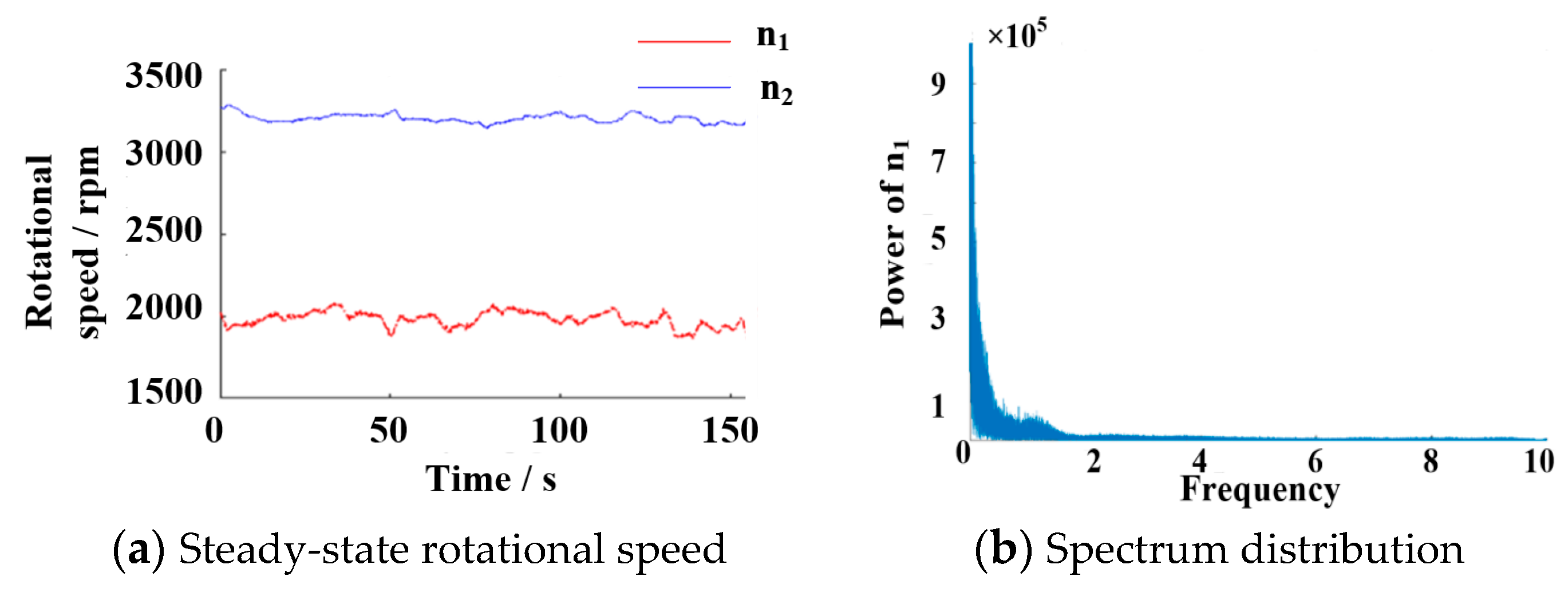
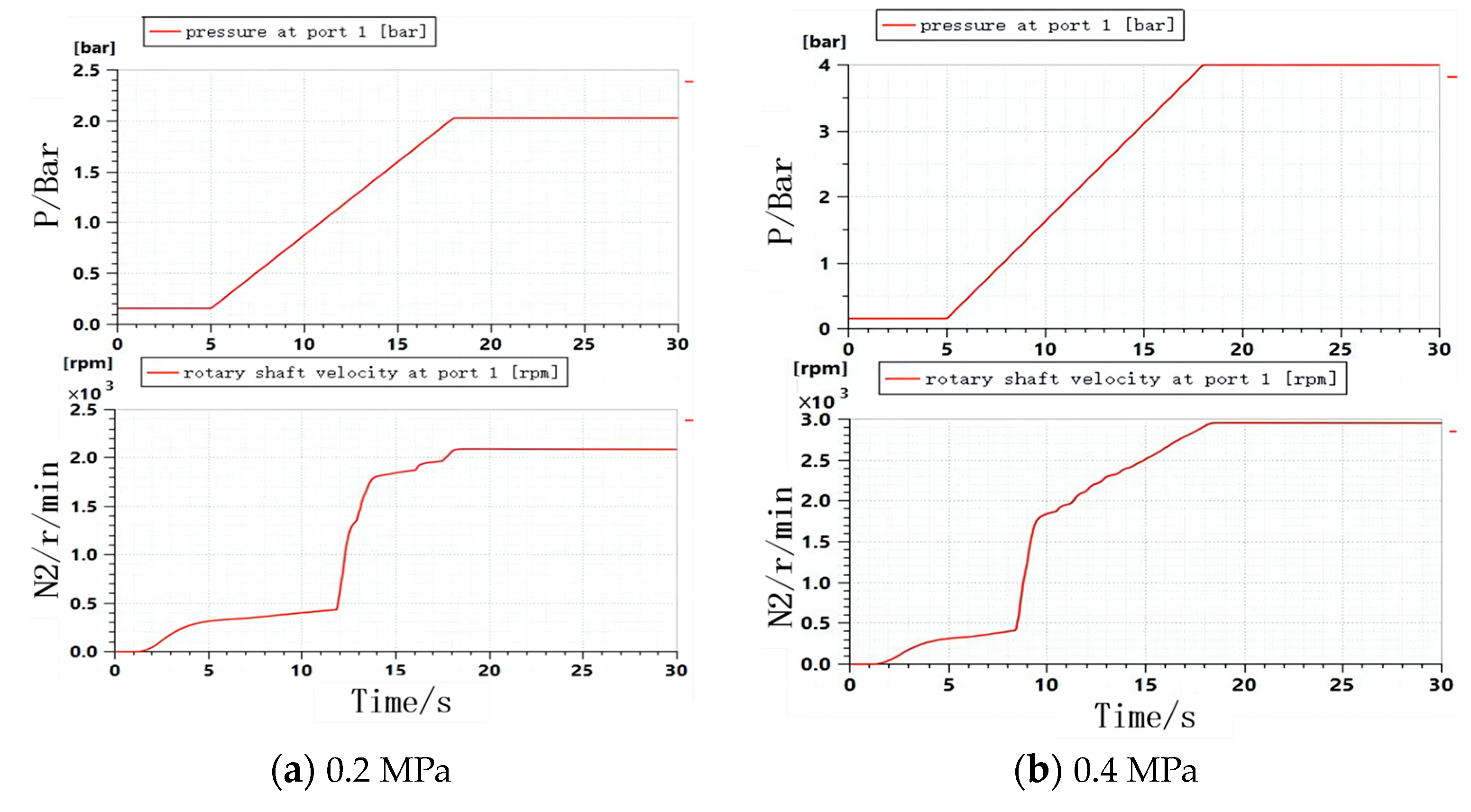
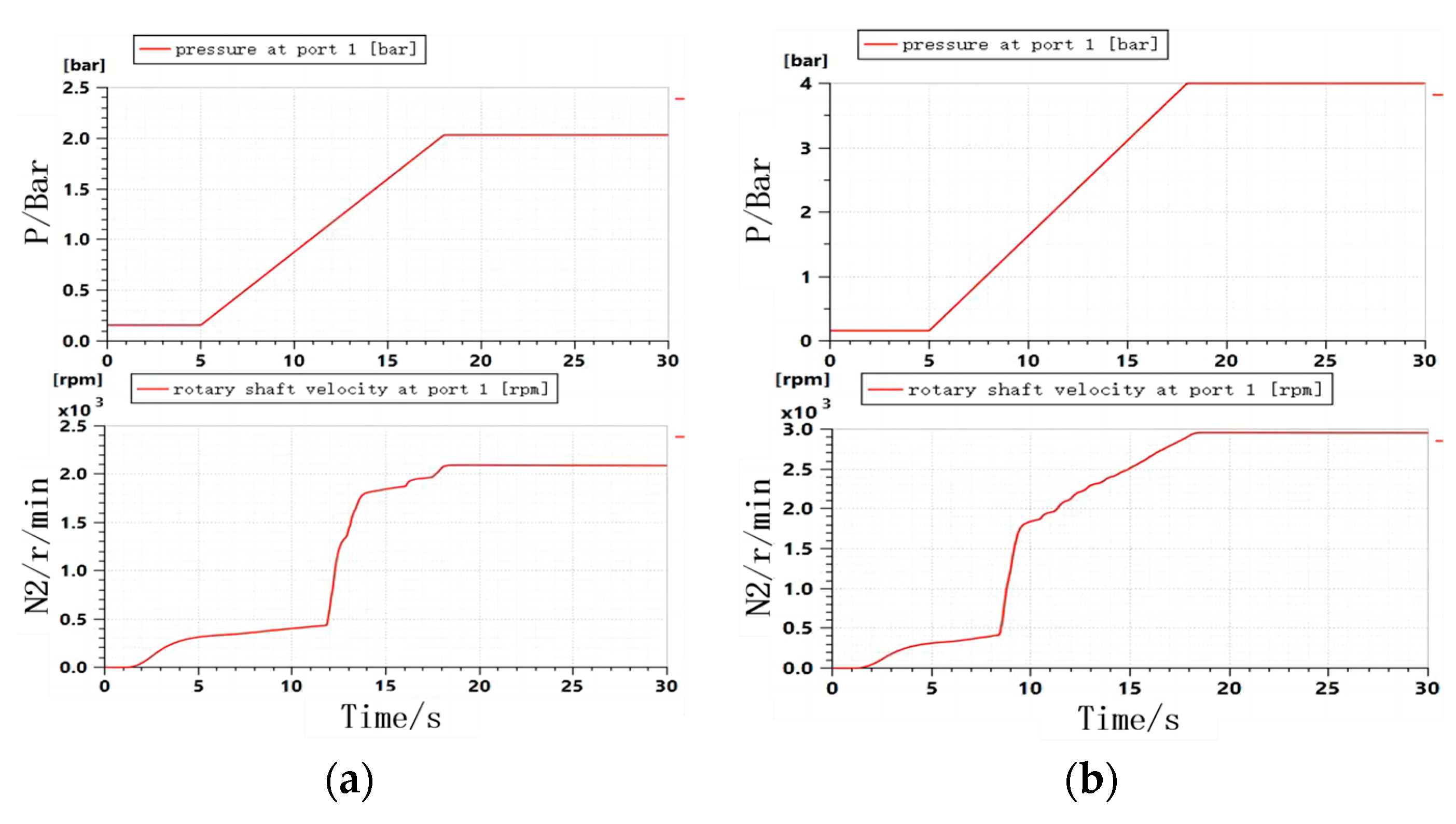
5.1. Steady-State Experiment Verification

5.1.1. Experiment Scheme

In the process of rotational speed control performance simulation, under different input rotational speeds and control modes (open loop and add inverse compensation control and double closed loop control of temperature and rotational speed), the control signal (unit percentage, linear corresponding proportional valve current) is slowly changed to simulate the steady-state relationship between the control signal and the output rotational speed. The input rotational speed range is 1500 rpm~4500 rpm; according to the input rotational speed, two rotational speeds are selected for the experiment: 2000 rpm and 4500 rpm. At each rotational speed gear, an open loop control experiment, feedforward compensation experiment with inverter ratio model, and double closed loop control experiment of temperature and rotational speed are carried out, respectively. The control signal with an output rotational speed curve is drawn, compared, and analyzed.

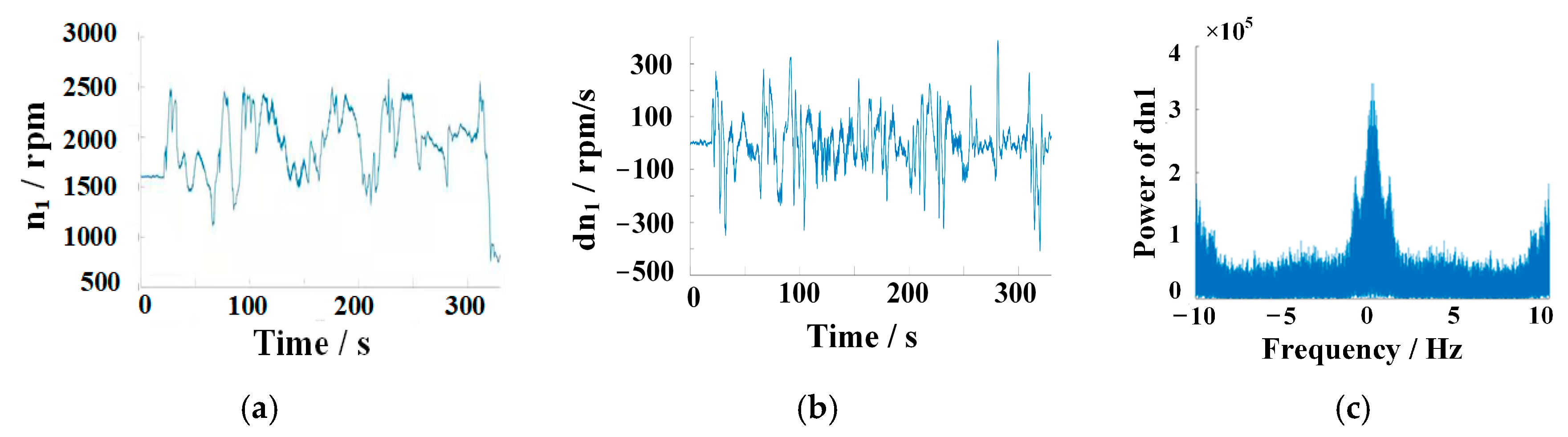
5.1.2. Experiment Results and Analysis

The simulating results of steady-state pressure control performance at different rotational speeds are shown in Figure 23 and Figure 24.

In Figure 24, the above simulations verify the effectiveness of the closed loop control method of rotational speed based on the combination of proportional model inverse compensation control and adaptive closed loop control. The simulating results show that the control method can effectively suppress the nonlinear characteristics of the HSCS and achieve better control effects. The comparison of steady-state speed control indices at 4500 rpm and 2000 rpm is shown in

Table 3. Steady-state indexes of comparison experiment when input rotational speed is 4500 rpm.

Evaluation Index	Open Loop Control	Feedforward Compensation	Double Closed Loop Control
Speed control domain of ascending phase	14~37%	3~35%	3~35%
Speed control domain of descending phase	0~21%	3~35%	3~35%
Effective speed control ratio	57~62%	86%	86%
Control hysteresis loop	43%	22%	14%
Nonlinearity of ascending phase	21%	19%	15%
Nonlinearity of descending phase	12%	10%	6%

and

Table 4. Steady-state indexes of comparison experiment when input rotational speed is 2000 rpm.

Evaluation Index	Open Loop Control	Feedforward Compensation	Double Closed Loop Control
Speed control domain of ascending phase	13~26%	2~25%	3~25%
Speed control domain of descending phase	0~17%	2~25%	3~25%
Effective speed control ratio	50~65%	88%	87%
Control hysteresis loop	39%	10%	5%
Nonlinearity of ascending phase	21%	8%	9%
Nonlinearity of descending phase	18%	9%	6%

.

The basic control conclusions that can be obtained are as follows:

(1)

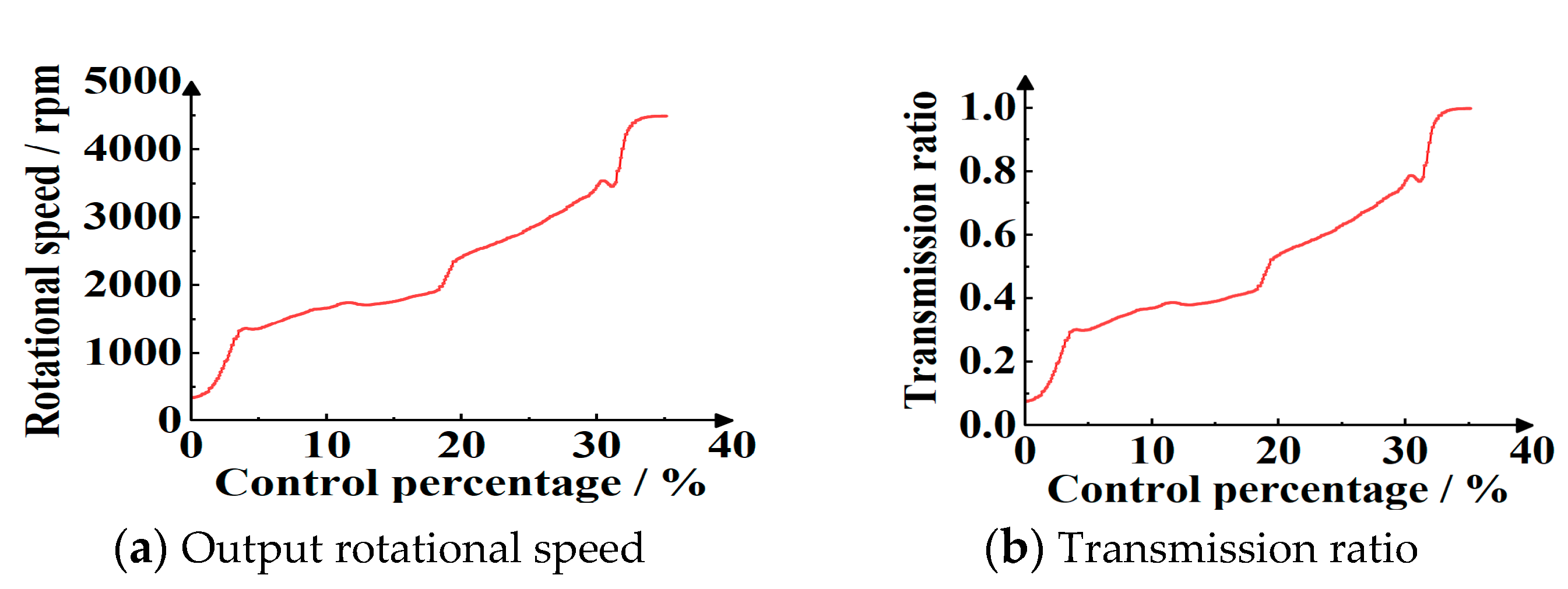
Equal ratio model inverse compensation control as a feedforward open loop control link can significantly reduce the open loop speed curve in the ascending and descending phases of the dead zone range and improve the sensitivity of the adjustment process while reducing hysteresis and nonlinearity also has a good effect.

(2)

The adaptive closed loop control is superimposed on the open loop feedforward control, which can further reduce the control hysteresis and nonlinearity, and can significantly improve the ability of disturbance rejection and adaptability of the model parameters change caused by oil temperature, input rotational speed, and other factors.

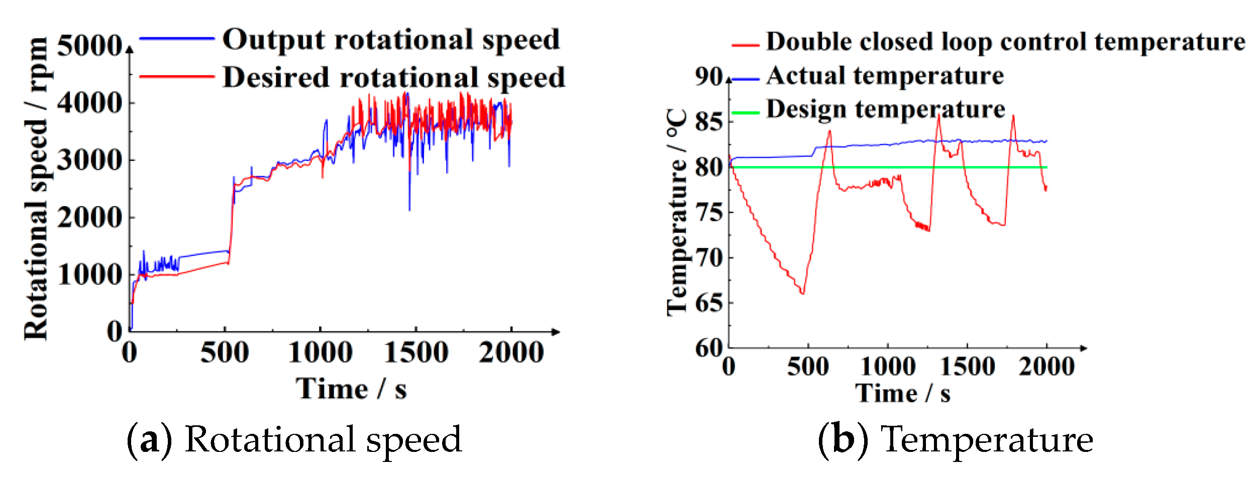
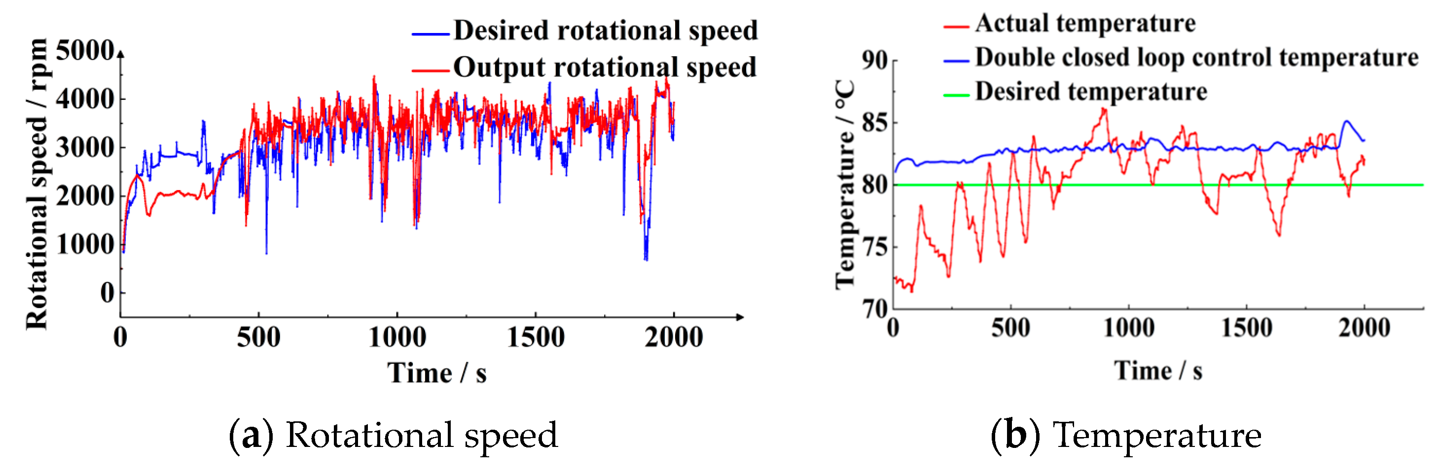
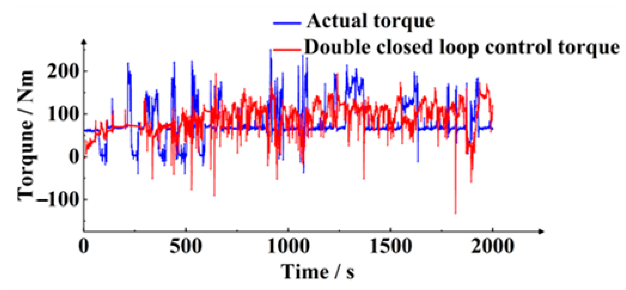
5.2. Experiment of Double Closed Loop Control of Temperature and Rotational Speed

5.2.1. Experiment Condition

The double closed loop control of temperature and rotational speed adopts semiphysical simulation. The temperature control process runs on the MATLAB R2021b/Simulink platform, and the temperature control model is used as the simulation control object. The rotational speed control runs in the speed controller, and HSCS on the bench is the control object. The closed loop of temperature control runs on the MATLAB R2021b/Simulink simulation platform, and the inner loop of rotational speed control runs on the bench simulating system.

Two typical conditions are extracted from the real vehicle data file, including engine rotational speed, fan rotational speed, transmission oil temperature, and water temperature, as the input parameters of the control process. The real vehicle condition acquisition curve is shown in Figure 25.

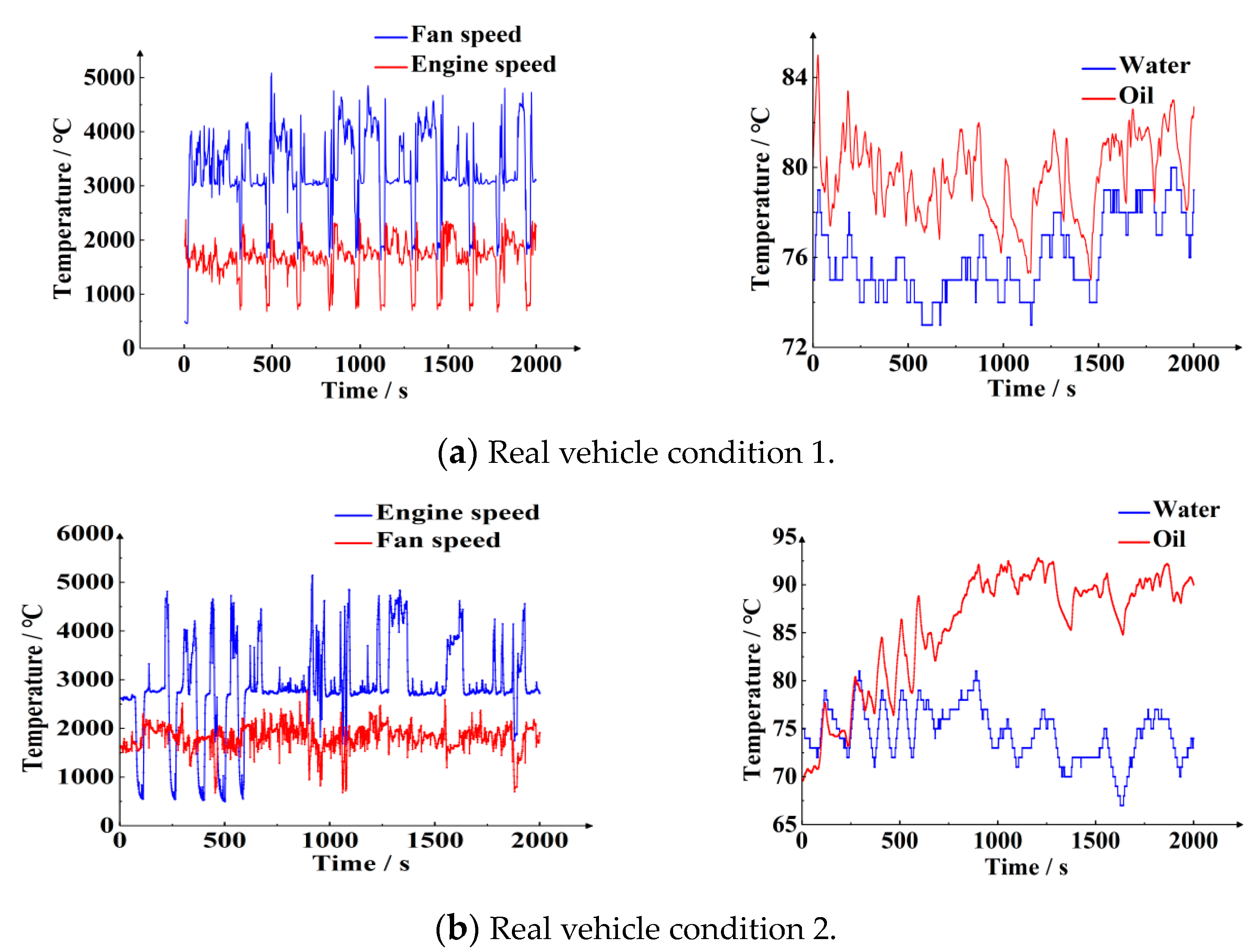
5.2.2. Real Vehicle Condition 1

The simulation results of double closed loop control of temperature and rotational speed under real vehicle condition 1 are shown in Figure 26 and Figure 27.

In Figure 26a, in the comparison curve of the desired rotational speed of the fan and the output rotational speed of the speed controller, the dark blue line is the desired rotational speed of the fan, and the dark red line is the output rotational speed of the rotational speed control. The output rotational speed of the speed controller can follow the changing trend of the desired rotational speed, but there is a tracking error, although it does not affect the temperature control effect.

In Figure 26b, in the comparison curve of the desired temperature, the simulation temperature, and the actual temperature, the red line is the desired temperature, the blue line is the temperature control curve of the double closed loop control, and the yellow line is the real vehicle temperature curve. Through the curve comparison, the MPC temperature control process fluctuates little, the control value is stable, and the error is 3.2 °C.

The comparison curve of the dynamic torque of the hydro-viscous shaft is shown in Figure 27.

In Figure 27, the red line is the dynamic torque curve of the hydro-viscous shaft under the double closed loop control of temperature and rotational speed, and the blue line is the dynamic torque curve of the real vehicle. By comparison, the double closed loop control of temperature and rotational speed significantly reduces the dynamic torque change range, and the dynamic torque change range decreases from 250 Nm to 155 Nm.

5.2.3. Real Vehicle Condition 2

The simulation results of double closed loop control of temperature and rotational speed under real vehicle condition 2 are shown in Figure 28.

In Figure 28, the output rotationalspeed can basically follow the changing trend of the desired speed, but there is a tracking error, although it does not affect the temperature control effect. MPC temperature control process fluctuation is very small, the control value is stable, and the error is 3.2 °C.

The comparison curve of the dynamic torque of the hydro-viscous shaft is shown in Figure 29. The red is the dynamic torque change curve of the hydro-viscous shaft under the double closed loop control of the temperature and rotational speed controller speed, and the blue is the dynamic torque curve of the real vehicle. It can be seen from the comparison that the double closed loop control of the temperature and rotational speed controller speed significantly reduces the dynamic torque change range, and the dynamic torque change range is reduced from 250 Nm to 200 Nm.

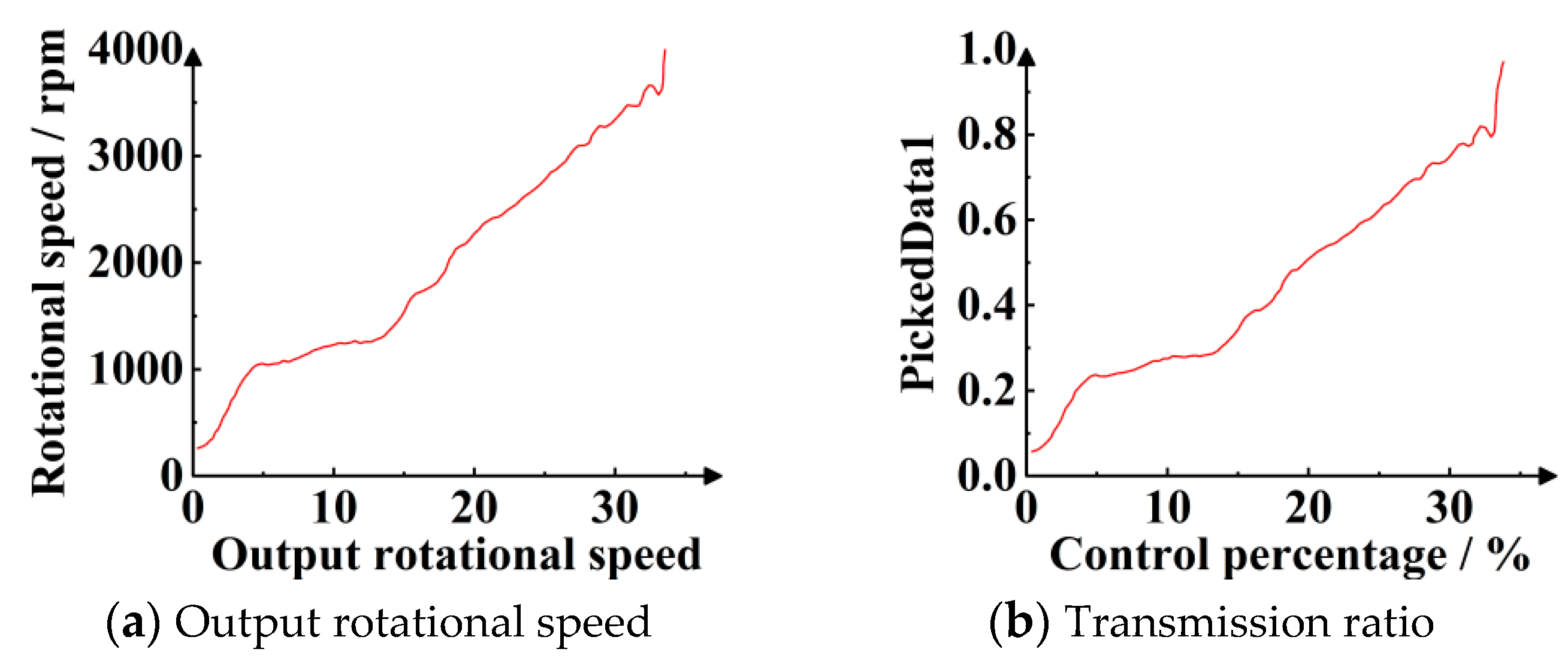
5.3. HSCS Domain Range Experiment

5.3.1. Experiment Scheme

The inlet oil temperature is set at 70 °C and 80 °C, and the input rotational speed of the hydro-viscous clutch is 4501 ± 50 r/min. The actual load of the fan is simulated to ensure that the load is 110 ± 20 Nm when the output rotational speed is 2500 ± 50 r/min and the load is 380 ± 20 Nm when the output rotational speed is 4501 ± 50 r/min.

The bench simulating controller is used to adjust the oil pressure, which increases slowly from zero pressure until the hydro-viscous clutch is fully combined (the input and output rotational speeds of the simulating piece are equal).

Draw and record the oil pressure–transmission ratio curve from the curve manually. Query the minimum transmission ratio and the maximum transmission as the speed range. Set the maximum hydro-viscous speed ratio to be greater than 0.8, the minimum value to be less than 0.2, and the simulation passes.

Stable output rotational speed n₂ is defined as the input rotational speed n₁, and control oil pressure remains unchanged when the output rotational speed fluctuation rate is less than 300 r/min, according to the following formula for calculating the transmission ratio.

$$i=\frac{n_2}{n_1}$$

(28)

5.3.2. Experiment Results and Analysis

The simulation data when the oil temperature is 70 °C are shown in Figure 30.

From the simulating curve in Figure 30, it can be calculated that the maximum stable rotational speed is 3688 r/min when the corresponding transmission ratio is 0.82, and the minimum stable rotational speed is 345 r/min when the corresponding transmission ratio is 0.07.

The simulating data when the oil temperature is 80 °C are shown in Figure 31.

From the simulating curve in Figure 31, it can be calculated that the maximum stable rotational speed is 3692 r/min when the corresponding transmission ratio is 0.82, and the minimum stable rotational speed is 291 r/min when the corresponding transmission ratio is 0.06.

The maximum and minimum of the transmission ratio of HSCS is 0.82 and 0.07, which satisfied the requirement.

6. Conclusions

In this paper, a novel control method of HSCS is studied, including the temperature closed loop control and the rotational speed closed loop control, and the two links are connected in series. Based on the double closed loop control with temperature closed loop and inner loop of rotational speed as the core, aiming at the problems of narrow speed control domain and poor disturbance rejection ability of HSCS, the temperature closed loop control with MPC as the core, and the closed loop control of rotational speed with feedforward compensation inverse hysteresis control and closed loop feedback of ADRC are completed. A novel double closed loop control method of temperature and rotational speed of integrated multi-parameter HSCS based on equal-ratio inverse compensation of data model is formed. The simulating program can complete the automatic comprehensive performance simulation of HSCS under different control parameters and realize the compound control mode of rotational speed closed loop and temperature closed loop. The effective transmission ratio under steady-state conditions is extended to 0.2~0.8, and the hydro-viscous torque and rotational speed fluctuation under engine rotational speed fluctuation are reduced by more than 30%. Through simulating verification, the novel control method of the HSCS designed in this paper can effectively improve the influence of input rotational speed and lubricating oil temperature on the rotational speed control performance of the HSCS and can effectively expand the domain of HSCS and speed control stability. It can be widely used in nonlinear HSCS, such as hydro-viscous clutches.

References

1. Meng, Q.R.; Hou, Y.F. Mechanism of hydro-viscous soft start of belt conveyor. J. China Univ. Min. Technol. Engl. Ed. 2008, 18, 7. [Google Scholar] [CrossRef]
2. Hou, Y.; Xie, F.; Huang, F. Control strategy of disc braking systems for downward belt conveyors. Min. Sci. Technol. China Univ. Min. Technol. 2011, 21, 491–494. [Google Scholar] [CrossRef]
3. Liao, X.; Yang, S.; Hu, D.; Gong, G. Analysis and revision of torque formula for hydro-viscous clutch. Energies 2021, 14, 103390. [Google Scholar] [CrossRef]
4. Cui, H.; Lian, Z.; Li, L.; Wang, Q. Analysis of influencing factors on oil film shear torque of hydro-viscous drive. Ind. Lubr. Tribol. 2018, 70, 1169–1175. [Google Scholar] [CrossRef]
5. Bullough, W.A.; Johnson, A.R.; Hosseini-Sianaki, A.; Makin, J.; Firoozian, R. Electro-rheological clutch: Design, performance characteristics and operation. Proc. Inst. Mech. Eng. Part I J. Syst. Control Eng. 1993, 207, 87–95. [Google Scholar] [CrossRef]
6. Meng, Q.R.; Hou, Y.F. Effect of oil film squeezing on hydro-viscous drive speed regulating start. Tribol. Int. 2010, 43, 2134–2138. [Google Scholar]
7. Xue, J.; Ma, B.; Chen, M.; Zhang, Q.; Zheng, L. Experimental investigation and fault diagnosis for buckled wet clutch based on multi-speed hilbert spectrum entropy. Entropy 2021, 23, 1704. [Google Scholar] [CrossRef] [PubMed]
8. Gong, G.; Wang, F.; Qin, Y.; Zhang, Y.; Sun, C.; Yang, H. The design of low cost valve-and-pump compounded pressure control system for the hydro viscous clutch. Mechatronics 2020, 65, 102310. [Google Scholar] [CrossRef]
9. Ahamed, R.; Ferdaus, M.M.; Li, Y. Advancement in energy harvesting magneto-rheological fluid damper: A review. Korea Aust. Rheol. J. 2016, 28, 355–379. [Google Scholar] [CrossRef]
10. Ma, L.G.; Xiang, C.L.; Zou, T.G.; Mao, F.H. Research on Control Strategy of Hydro-Viscous Driven Fan Cooling System. Appl. Mech. Mater. 2014, 722, 182–189. [Google Scholar] [CrossRef]
11. Ding, H.; Zhao, J. A new method of improving low-speed performance of variable speed hydraulic systems: By leaking parallel valve control. Adv. Mech. Eng. 2014, 2014, 967373. [Google Scholar] [CrossRef]
12. Ferreira, F.J.; Fong, J.A.; de Almeida, A.T. Ecoanalysis of variable-speed drives for flow regulation in pumping systems. IEEE Trans. Ind. Electron. 2011, 58, 2117–2125. [Google Scholar] [CrossRef]
13. Lamaddalena, N.; Khila, S. Energy saving with variable speed pumps in on-demand irrigation systems. Irrig. Sci. 2012, 30, 157–166. [Google Scholar] [CrossRef]
14. Cui, J.; Li, H.; Zhang, D.; Xu, Y.; Xie, F. Multi-objective optimization of hydro-viscous flexible drive for dynamic characteristics using genetic algorithm. Ind. Lubr. Tribol. 2021, 73, 1003–1010. [Google Scholar] [CrossRef]
15. Qi, H.; Liu, S.; Yang, R.; Yu, Y. Research on new intelligent pump control based on sliding mode variable structure control. In Proceedings of the 2017 IEEE International Conference on Mechatronics and Automation, ICMA 2017, Takamatsu, Japan, 6–9 August 2017; pp. 1239–1244. [Google Scholar]
16. Yin, X.X.; Lin, Y.G.; Li, W.; Gu, H.G. Hydro-viscous transmission based maximum power extraction control for continuously variable speed wind turbine with enhanced efficiency. Renew. Energy 2016, 87, 646–655. [Google Scholar] [CrossRef]
17. Jahmeerbacus, M.I. Flow rate regulation of a variable speed driven pumping system using fuzzy logic. In Proceedings of the 2015 4th International Conference on Electric Power and Energy Conversion Systems, EPECS 2015, Sharjah, United Arab Emirates, 24–26 November 2015; pp. 1–6. [Google Scholar]
18. Kastrevc, M.; Puenjak, R. Fuzzy pressure control of hydraulic system with gear pump driven by variable speed induction electro-motor. Exp. Tech. 2005, 29, 57–62. [Google Scholar] [CrossRef]
19. Ye, Y.; Yin, C.-B.; Gong, Y.; Zhou, J.-j. Position control of nonlinear hydraulic system using an improved PSO based PID controller. Mech. Syst. Signal Process. 2017, 83, 241–259. [Google Scholar] [CrossRef]
20. Liang, H.; Zou, J.; Zuo, K.; Khan, M.J. An improved genetic algorithm optimization fuzzy controller applied to the wellhead back pressure control system. Mech. Syst. Signal Process. 2020, 142, 106708. [Google Scholar] [CrossRef]
21. Ji, Y.; Zhang, J.; He, C.; Ma, R.; Hou, X.; Hu, H. Constraint performance pressure tracking control with asymmetric continuous friction compensation for booster based brake-by-wire system. Mech. Syst. Signal Process. 2022, 174, 109083. [Google Scholar] [CrossRef]
22. Lu, J.; Xie, H.; Hu, L.; Yang, H.; Chen, Y. Variable-parameter feedforward control for centrifuge shaking table based on nonlinear frequency characteristic model. Mech. Syst. Signal Process. 2021, 161, 108011. [Google Scholar] [CrossRef]
23. Song, Y.H.; Ba, K.X.; Wang, Y.; Zhang, J.X.; Yu, B.; Zhang, Q.W.; Kong, X.D. Study on nonlinear dynamic behavior and stability of aviation pressure servo valve-controlled cylinder system. Nonlinear Dyn. 2022, 108, 3077–3103. [Google Scholar] [CrossRef]
24. Zhu, Q.; Huang, D.; Yu, B.; Ba, K.; Kong, X.; Wang, S. An improved method combined SMC and MLESO for impedance control of legged robots’ electro-hydraulic servo system. ISA Trans. 2022, 130, 598–609. [Google Scholar] [CrossRef] [PubMed]
25. Chen, Z.; Li, J.; Wang, J.; Wang, S.; Zhao, J.; Li, J. Towards Hybrid Gait Obstacle Avoidance for a Six Wheel-Legged Robot with Payload Transportation. J. Intell. Robot. Syst. 2021, 102, 60. [Google Scholar] [CrossRef]
26. Zhan, G.; Zhang, Z.; Chen, Z.; Li, T.; Wang, D.; Zhan, J.; Yan, Z. Stewart-inspired parallel spatial docking robot: Design, analysis and experimental results. Robot. Intell. Autom. 2023, 43, 313–326. [Google Scholar] [CrossRef]
27. Ba, K.X.; Liu, G.J.; Ma, G.L.; Chen, C.H.; Pu, L.Y.; He, X.L.; Chen, X.; Wang, Y.; Zhu, Q.X.; Wang, D.K. Bionic perception and transmission neural device based on a self-powered concept. Cell Rep. Phys. Sci. 2024, 5, 102048. [Google Scholar] [CrossRef]
28. Huang, Y.; Meng, Z.; Sun, J. Scalable distributed least square algorithms for large-scale linear equations via an optimization approach. Automatica 2022, 146, 110572. [Google Scholar] [CrossRef]
29. Ruder, S. An overview of gradient descent optimization algorithms. arXiv 2016, arXiv:1609.04747. [Google Scholar]
30. Fang, Y.; Mo, H. Slope Stability Analysis Based on The Memoryless Least Square Quasi-Newton Method. Chin. J. Rock Mech. Eng. 2002, 21, 34–38. [Google Scholar]
31. Taherkhorsandi, M.; Castillo-Villar, K.K.; Mahmoodabadi, M.J.; Janaghaei, F.; Mortazavi Yazdi, S.M. Optimal Sliding and Decoupled Sliding Mode Tracking Control by Multi-objective Particle Swarm Optimization and Genetic Algorithms. In Advances and Applications in Sliding Mode Control Systems; Springer International Publishing: Cham, Switzerland, 2015. [Google Scholar] [CrossRef]
32. Zhang, S.; Xu, H.; Zhang, H.; Yang, S. Game-relationship-based remanufacturing scheduling model with sequence-dependent setup times using improved discrete particle swarm optimization algorithm. Concurr. Eng. Res. Appl. 2022, 30, 424–441. [Google Scholar] [CrossRef]
Figure 1. The overall control strategy block diagram of HSCS.
Machines 12 00394 g001
Figure 2. Main loop and secondary loop phenomena of HSCS.
Machines 12 00394 g002
Figure 3. Input and output rotational speed running-in curve.
Machines 12 00394 g003
Figure 4. Steady-state condition analysis.
Machines 12 00394 g004
Figure 5. The running-in curve and speed change rate fluctuation curve. (a) Engine rotational speed running-in curve. (b) Rotational speed change rate fluctuation curve. (c) Spectrum analysis of engine dynamic condition.
Machines 12 00394 g005
Figure 6. The steady-state curves of HSC at different oil temperatures. (a) Steady-state curves under different lubricating oil temperatures. (b) Variation curve of lubricating oil temperature-drag rotational speed.
Machines 12 00394 g006
Figure 7. Strategy block diagram of data modeling.
Machines 12 00394 g007
Figure 8. Comparison curve of training model and actual data. (a) Input rotational speed is 1500 rpm. (b) Input rotational speed is 3000 rpm.
Machines 12 00394 g008
Figure 9. Diagram of main loop, secondary loop, and mapping method.
Machines 12 00394 g009
Figure 10. Steady speed control curves at different input rotational speeds.
Machines 12 00394 g010
Figure 11. Steady-state speed control curves at different oil temperatures.
Machines 12 00394 g011
Figure 12. Principle of temperature control based on MPC.
Machines 12 00394 g012
Figure 13. Variation curves of temperature of water, oil, and oil–water of real vehicle.
Machines 12 00394 g013
Figure 14. Basic principle and implementation process of MPC.
Machines 12 00394 g014
Figure 15. Schematic diagram for the temperature control principle in HSCS.
Machines 12 00394 g015
Figure 16. Block diagram of operation logic of particle swarm algorithm.
Machines 12 00394 g016
Figure 17. Experimental curve of oil pressure and rotational speed when oil temperature is 70 °C.
Machines 12 00394 g017
Figure 18. Simulating curves of oil pressure and rotational speed when oil temperature is 70 °C.
Machines 12 00394 g018
Figure 19. Experimental curve of oil pressure and rotational speed when oil temperature is 80 °C.
Machines 12 00394 g019
Figure 20. Simulating curves of oil pressure and rotational speed when oil temperature is 80 °C.
Machines 12 00394 g020
Figure 21. Block diagram of closed loop control of HSCS.
Machines 12 00394 g021
Figure 22. Construction of ADRC.
Machines 12 00394 g022
Figure 23. Comparison of different control strategies when input rotational speed is 4500 rpm.
Machines 12 00394 g023
Figure 24. Comparison experiment of different controls when input rotational speed is 2000 rpm.
Machines 12 00394 g024
Figure 25. Two typical conditions of real vehicles.
Machines 12 00394 g025
Figure 26. Comparison curves of rotational speed and temperature.
Machines 12 00394 g026
Figure 27. Comparison curves of dynamic torque.
Machines 12 00394 g027
Figure 28. Contrast curves of rotational speed and temperature.
Machines 12 00394 g028
Figure 29. Comparison curves of dynamic torque of hydro-viscous shaft.
Machines 12 00394 g029
Figure 30. Simulating curves of rotational speed range when oil temperature is 70 °C.
Machines 12 00394 g030
Figure 31. Simulating curves of rotational speed range when oil temperature is 80℃.
Machines 12 00394 g031