Article

A Fault Prediction Method for CNC Machine Tools Based on SE-ResNet-Transformer

1
School of Mechanical and Electrical Engineering, Qiqihar University, Qiqihar 161006, China
2
The Engineering Technology Research Center for Precision Manufacturing Equipment and Industrial Perception of Heilongjiang Province, Qiqihar 161006, China
*
Author to whom correspondence should be addressed.
Machines 2024, 12(6), 418; https://doi.org/10.3390/machines12060418
Submission received: 6 May 2024 / Revised: 23 May 2024 / Accepted: 14 June 2024 / Published: 18 June 2024

Abstract

:
Aiming at the problem that predicted data do not reflect the operating status of computer numerical control (CNC) machine tools, this article proposes a new combined model based on SE-ResNet and Transformer for CNC machine tool failure prediction. Firstly, the Transformer model is utilised to build a non-linear temporal feature mapping using the attention mechanism in multidimensional data. Secondly, the predicted data are transformed into 2D features by the SE-ResNet model, which is adept at processing 2D data, and the spatial feature relationships between predicted data are captured, thus enhancing the state recognition capability. Through experiments, data involving the CNC machine tools in different states are collected to build a dataset, and the method is validated. The SE-ResNet-Transformer model can accurately predict the state of CNC machine tools with a recognition rate of 98.56%. Results prove the effectiveness of the proposed method in CNC machine tool failure prediction. The SE-ResNet-Transformer model is a promising approach for CNC machine tool failure prediction. The method shows great potential in improving the accuracy and efficiency of CNC machine tool failure prediction. Feasible methods are provided for precise control of the state of CNC machine tools.

1. Introduction

With the development of mechanized massive production, the degree of automation and complexity of mechanical systems is increasing. Under the influence of severe operating conditions such as variable loads, strong excitation, and large disturbances, mechanical components will inevitably produce a degradation of performance and health status during long-term service, eventually leading to failure. The ability to predict the future operating status of CNC machine tools allows for the identification of potential abnormal emergencies, thereby reducing the risk of losses incurred as a result of the failure of the production process. Furthermore, it enhances the stability of the machine tool processing and serves as a valuable reference in the repair and maintenance of the equipment [1]. Currently, the field of CNC machine tool failure diagnosis is starting to use deep learning techniques that are good at feature learning and pattern recognition [2]. Many researchers have made significant contributions to local data prediction and fault identification in CNC machine tools [3,4,5,6,7,8,9].
In the area of data forecasting, there are two main approaches in data prediction, including long short-term memory (LSTM) networks and Transformer networks. Deng et al. proposed a Conv-LSTM-Transformer network model and extracted low-dimensional spatial features through the Conv-LSTM network [10]. They clarified the direct mapping rules between nonlinear spatiotemporal feature formation and equipment service performance degradation using the attention mechanism in Transformer. In the field of bearing life prediction, Sun et al. also introduced a Transformer self-attention transfer network structure and extracted the key time-varying information from a high-dimensional dataset with the model while retaining all information in data transformation. Experimental validation of this model was conducted on the FEMTO-ST bearing dataset, which showed it achieved a leading position in bearing life prediction [11]. In the context of wind turbine fault prediction and short-term load forecasting, LSTM networks were combined with CNNs and recurrent neural networks (RNNs) to explore the temporal correlations of different data points in a time series [12,13]. The two approaches differ in early feature extraction. RNNs focus on the relationships of individual data points in a time series, emphasizing the extraction of features from a single data time series, and thus are more suitable for individual data prediction scenarios. CNNs extract features through convolution and perform well in 2D images, showing higher accuracy in processing multiple types of data simultaneously.
In the field of fault classification, many researchers adopt neural networks. Yu et al. presented a cascaded monitoring network method to develop a monitoring model with concurrent analytics of temporal and spatial information and extracted both temporal and spatial information by performing a convolution operation on the variables. Sub-models were developed for each convolutional feature to generate a monitoring model. The proposed method can effectively detect abnormal samples in industrial processes and accurately isolate faulty variables from normal ones [14]. Yu et al. proposed several methods for industrial process fault detection. Broad convolutional neural networks (BCNNs) have been proposed for fault identification. Broad CNN models can enhance the learning capability by adding newly generated additional features, so that BCNN models can self-update to include new coming abnormal samples and fault classes [15,16]. Wang et al. proposed a novel spate-temporal feature fusion network, in which the spate-temporal features of the signal were enhanced and then extracted for fault identification [17]. Residual networks are used in classification tasks in several domains. Yu et al. employed a residual network for fault diagnosis in pipeline robots, which takes vibration signals as feature inputs, extracts potential features, and performs classification [18]. Residual networks can significantly improve the classification performance and are more suitable for deployment in embedded setups because of low computational requirements. Incorporating the squeeze-and-excitation (SE) module into neural networks is more advantageous for obtaining fault-related target information. Lu et al. performed power system fault classification by integrating SE modules into the DarkNet37 network [19]. The network can acquire more fault-related target information by recalibrating the weights of the important information channels with the SE module. These results demonstrate an accuracy of 97.22%, which represents a significant improvement over the network without the SE module.
In time series data, one-dimensional data may not fully capture the interconnections between time points. Therefore, Quan et al. transformed one-dimensional data into two-dimensional data and then enhanced the data features by fusing the two types of data [20]. This processing method can more effectively extract features. In the field of 2D image recognition dominated by CNNs, residual networks are prominent. Gao et al. proposed a texture image that arranged the time domain signal according to the features of the frequency domain and converted the features of the signal into a texture image that was more suitable for 2D convolution kernel extraction. This method offers a solution to the issue of individual channel data being unable to accurately reflect fault characteristics. The utilization of texture images within the dataset enables the method to be 100% accurate [21]. Fu et al. used the SDP method to convert the vibration signal of a single multi-channel sensor into an imaging arm. The image arm in question contains information pertaining to a multitude of channels. Both single-channel fault diagnosis and multi-channel diagnosis accuracy were improved, and the accuracy of the multi-channel diagnosis after fusion was also mostly higher than the accuracy of single-channel diagnosis after fusion when the fusion theory was used [22].
This study proposes a CNC machine tool fault prediction method that combines SE-ResNet and Transformer. SE-ResNet has significant advantages in feature representation [23]. Transformer is good at sequence processing [24]. This approach is aimed at enhancing the accuracy and real-time performance of fault detection by leveraging the strengths of both models. Experimental validation demonstrates a significant improvement in performance compared to the existing techniques and thereby proves the effectiveness and feasibility of the proposed method in complex industrial environments.
The main contributions of this article are listed as follows:
1.
In this study, the Transformer model and SE-ResNet model are used jointly. The state classification module was added after the data prediction module to efficiently and accurately complete the classification of predicted fault data.
2.
The spatial connections between different predicted feature data are improved through two-dimensional data fusion. The data fusion module combines the independent data. This approach allows not only temporal but also spatial features to be extracted during the convolution operation. This transforming enables cross-data feature extraction and recognition, thereby strengthening the identification capability of this method.
3.
A dataset is established by simulating different states of CNC machine tools through experimental simulations. The proposed method is experimentally validated on the dataset, achieving a prediction accuracy of 98.56%. The effectiveness of the proposed method is thus validated.
The rest of the paper is structured as follows. The Transformer, SE-ResNet, and SE-ResNet-Transformer networks are briefly described in Section 2. Experimental validation results and comparison analyses are illustrated in Section 3. Finally, conclusions are composed in Section 4.

2. The Proposed Method

This section will introduce the SE-ResNet-Transformer model for CNC machine tool fault prediction. The proposed method is a novel deep learning architecture that combines the advantages of SE-ResNet and Transformer models.

2.1. SE-ResNet-Transformer Model

The SE-ResNet-Transformer model integrates the structures of SE-ResNet and Transformer. It is primarily composed of a Transformer, a classification module, and a data transformation module (Figure 1). The SE-ResNet-Transformer model contains an encoder and a decoder. The encoder is further divided into multi-head attention modules and feed-forward neural network layers. Residual connections exist between the two sub-functions, which are followed by normalization operations. The encoder comprises three function layers with identical structures, and each layer consists of three sub-function layers. The first layer is identical to the sub-function layer of the encoder. The second layer modifies the attention layer by adding a masking component on the top of the sub-function layer of the encoder to ensure that the prediction results at a certain position only depend on the preceding outputs at that position. The third layer applies a multi-head attention mechanism to the output of the encoder. All three layers contain residual structures. An image transformation process is introduced between the two models to convert the one-dimensional data predicted by the prediction module into two-dimensional data, which are then inputted into the classification module. In each residual module, a convolution operation is first conducted. Next, the features are batch-normalized to optimize the network performance. Nonlinearity is introduced to the network through ReLU activation functions. After two convolution operations, an SE module branch is expanded for recognizing important features. Certain weights are assigned to the important features, and less important features are ignored. This step is performed in addition to the normal downward branch combined with the residual structure. The weight parameters obtained by the SE module are then weighted to the residual operation results to recalibrate the features obtained by the residual structure. This step enhances the role of effective features in fault classification. In summary, the SE-ResNet-Transformer model adopts a fusion of two models and integrates the previous sole prediction and information classification. Through predictions, this model can pre-emptively discern the subsequent state, gaining insights into future information. This process enables the control of future information from the present moment and transforms abnormal future information into normal future information. The detailed information about each module of the model is provided below.
The architecture representing the sequential steps in the proposed method is illustrated in Figure 2. The method employs the Transformer model, starting from signal acquisition, and captures relevant features. Nonlinear temporal features in multidimensional time series data are also captured. Thereby, the required feature data are predicted. Subsequently, the feature data are transformed into two-dimensional data, which are then inputted into the SE-ResNet model for state determination. This method combines the expertise of SE-ResNet in processing two-dimensional images and the expertise of Transformer in processing one-dimensional time series data, thereby enhancing the strengths of both technologies and enabling the prediction of CNC machine tool states. SE-ResNet is particularly suitable for extracting spatial features from two-dimensional signal data, and Transformer can capture long-range temporal dependencies, thus making accurate fault predictions. The specific steps are shown as follows:
(1)
On-site experiments are conducted, where workpieces are processed to simulate four states, including a normal condition and three abnormal conditions. As a result, four scenarios and data from nine channels are generated and used to construct a CNC machine tool status dataset. The dataset is randomly partitioned into training and testing sets.
(2)
After data collection, the data are preprocessed to integrate data trend transformations, enabling the extraction of data trends under different states.
(3)
An SE-ResNet-Transformer model is established and trained using the training set. The CNC machine tool status data are used as the input to the SE-ResNet-Transformer model, and the predicted CNC machine tool status is the output. The data are processed through an encoder-decoder, and a classifier is employed to identify specific operating states.
(4)
The trained SE-ResNet-Transformer model is used to predict the CNC machine tool operating states. The actual and predicted CNC machine tool operating states are compared to evaluate the model.
The following sections will provide a more detailed overview of the proposed method.

2.2. SE-ResNet

2.2.1. Squeeze-and-Excitation (SE)

The attention mechanism is capable of directing attention to crucial areas and thereby facilitates the acquisition of more valuable and critical information [25]. With regard to the multi-channel data of CNC machine tools, different types of data change to varying degrees in accordance with the processing state. Consequently, their contributions to the classification results are naturally disparate. Though spatial attention mechanisms are used to assign distinct weights to distinct data, more emphasis is placed on the motor current, which contributes more significantly to the classification results. As a result, the degree of classification accuracy is improved. The principle of the SE module is illustrated in Figure 3.
The input X is mapped to U R H × W × C through a convolution transformation F t r and further refined to obtain recalibrated features through three main operations. (1) Squeeze: Feature U is compressed to F s q ( · ) through a squeezing operation, which compresses spatial dimension features into overall features and provides global feature information to a certain extent. (2) Excitation: The excitatory operation F s ( · , W ) adjusts the weights of different channels. (3) Scale: After the excitation operation, the weights between different channels, namely, the importance of different channels, are obtained. Recalibration of the original features is completed by updating the weights in this way, enhancing the model ability to recognize different feature channels.

2.2.2. ResNet

ResNet is a CNN proposed to address the performance degradation caused by excessively deep networks [26]. CNNs extract hierarchical features of image spatial features through a series of convolution and pooling operations. The local receptive field mechanism and weight-sharing characteristics of convolutional layers significantly reduce the number of parameters in the network. The pooling layer ensures that the features extracted by the convolutional layer have scale invariance, thereby improving the generalization ability of the network. As a type of residual network, ResNet introduces skip connections between network layers, where the output of the previous layer is directly added to the input of the subsequent layer. This technique enhances the representational capability of the network. The mathematical expression for the residual block is as follows:
F x = f x + x
where f x represents the transformation function of the residual block, x is the input, and F x is the output. F x is obtained by directly adding x with f x .
Structurally, the residual module adds the input to the output features (Figure 4), ensuring the output of the residual block contains both the transformed features and the original features. This step helps prevent the loss of feature values caused by excessive convolutional operations.

2.2.3. SE-ResNet

The introduction of the SE module into the ResNet structure results in SE-ResNet. The addition of the SE module enables ResNet to learn the weighting parameters of the channels and thus facilitates weighted processing between different types of data. The network structure is illustrated in Figure 5. The network of choice is SE-ResNet50, with the parameters listed in Table 1. Convolution and pooling operations are performed after the image enters the network. The primary structure of the network is constituted by combining multiple convolutional layers and SE modules. The methodology employed to calculate the primary module is as follows:
F x = x + C o n v x + S E C o n v x ,
where x denotes the input, C o n v ( x ) denotes the convolution operation, and S E ( x ) denotes the recalibration of the data by the SE module according to the parameters.
The main module has three types of data circulation, including raw data (x), convolutional data (Conv(x)), and recalibrated convolutional data (SE(Conv(x))). The raw data retain the original features through the residual structure. The convolutional data extract new features through convolutional operations. The recalibrated data calibrate the important features from the convolution operation. At the output of the main module, the three types of data are combined, retaining the original features and the newly extracted features. After these processes, a larger weight is assigned to the important data, reducing the influence of unimportant or redundant channel data on the classification results. After the extraction of the features, the data are subjected to an average pooling operation, which serves to reduce data dimensionality. The data are then entered into the fully connected layer and the Softmax layer, where the data are normalized to form the final output.

2.3. Transformer Model

Transformer is developed in the field of natural language processing. Before the advent of Transformer, RNNs and their variants were the main methods for processing sequential data, including LSTM and gated recurrent units. These models capture temporal dependencies by processing input sequences element by element, but they encounter challenges such as vanishing or exploding gradients and difficulties in parallel computation. The advent of Transformer addresses the limitations of LSTM, including the inability to train in parallel and the necessity to retain the entirety of the sequence information. The Transformer model is founded on the self-attention mechanism, which draws inspiration from the human cognitive system. This mechanism enables the model to direct its focus towards crucial elements of information while disregarding irrelevant details. The introduction of self-attention enables the Transformer model to establish direct dependency between any two positions, focusing on different subspaces of information at different positions. This function extends the model capability to attend to different features, thereby improving computational efficiency and model performance [27].
The Transformer model architecture features an encoder-decoder structure (Figure 6). The model includes an equal number of encoders and decoders.
Each encoder comprises multiple identical layers, each containing two sub-layers. The first sub-layer is a multi-head self-attention mechanism, and the second sub-layer is a simple position-wise fully connected feed-forward network. Each sub-layer is followed by a residual connection and layer normalization. Similarly, each decoder comprises multiple identical layers, each of which contains three sub-layers. The decoder has a third sub-layer, which retrieves the outputs from the encoder and processes them using the self-attention mechanism.
The model involves two crucial attention mechanisms.
In the context of self-attention mechanisms, the input dimensions are divided into queries, keys, and values. The information obtained by querying the keys is scaled by dividing by d K , and the weights of the values are obtained using SoftMax. Simultaneously, the attention function is queried and packed into matrix Q, and the keys and values are compressed into matrices K and V, respectively. The calculation formula is as follows:
A t t e n t i o n ( Q , K , V ) = s o f t m a a x Q K T d K V
In Figure 7, the multi-head attention mechanism operates by computing multiple self-attention mechanisms in parallel. This process involves projecting queries, keys, and values h times to obtain the values of dimension d K and d K , d v , respectively. Subsequently, attention is applied in parallel to each query, key, and value, resulting in an output of dimension d v . Next, the dimension values are linearly transformed through projection. The advantage of this model over single-head attention lies in its capacity to incorporate expression information from different positions.
The calculation formula for the multi-head attention mechanism is as follows:
M u l t i H e a d ( Q , K , V ) = C o n c a t ( h e a d 1 , h e a d 2 , , h e a d h ) W O   h e a d h = A t t e n t i o n ( Q W i Q , K W i K , V W i V ) ,
where the projections are parameter matrices W i Q R d m o d e l x d K , W i K R d m o d e l x d K , W i V R d m o d e l x d v , and W i 0 R h d V x d m o d e l .

2.4. Data Fusion

The transformer model outputs one-dimensional data, whereas SE-RESNET is adept at handling two-dimensional data. One-dimensional data contain temporal features before and after the event, and it is not possible to detect the features embedded between different kinds of data. Therefore, a data fusion module is added between the two models. This module combines multiple one-dimensional data into two-dimensional data. As a result of this operation, each piece of information contains both temporal and spatial features. Consequently, the method is better equipped to make state judgements [28].
The study did not transform the raw data in order to avoid any potential impact on the accuracy of the data. In order to extract sufficient spatial features, the study did not overlap code the data. The method employs RGB coding. Different kinds of data were combined, and the combination is shown in Figure 8.

2.5. Workflow of SE-ResNet-Transformer Model

The data flow during the operation of the fault prediction model (SE-ResNet-Transformer) is illustrated in Figure 9. The predictive model processes three types of monitoring data, each with three channels: current, temperature, and vibration. The three types of data in question comprise a total of nine channels, which are arranged vertically to form a data shape of 9 × N. In the prediction model, a sliding window is employed to collect data, thereby increasing the number of data samples. Subsequently, the data are extracted and subjected to a self-attention operation. During this operation, each data point is subjected to three distinct operations, forming matrices Q, K, and V. Matrix Q is multiplied separately with matrices K and V generated by itself and the sequential data, resulting in matrix QKV. Then, all matrices QKV generated by sequential data are normalized to obtain the relationship weight parameters between the original data and the sequential data. These steps complete the self-attention mechanism for a single feature. Then, the same operation is performed between different features to obtain weight parameters and complete the self-attention mechanism. Subsequently, the data are fed into the decoder, which employs a hidden multi-head attention mechanism for processing. In accordance with the pattern of the input data during training, the decoder obtains the occurrence probability of each data sequence. The data are inputted into the fully connected layer and are used to predict data based on the probability between sequential data. These steps complete the predictive data function of the model, and the next step is to classify the states using SE-ResNet.
The data conversion module is joined between the two sub-models and converts the predicted data into images. After the conversion, the nine channels of data are aligned in the chronological order. The time-aligned data are converted to a 9 × 9 image in the form of a sliding window. The prediction data are transformed into 2D matrix data, which are then fed into the SE-ResNet model. Firstly, the SE-ResNet model performs a convolution operation on the image information in order to extract features. Then, the features are identified using the training model, forming a CNC machine tool state.

3. Experimental

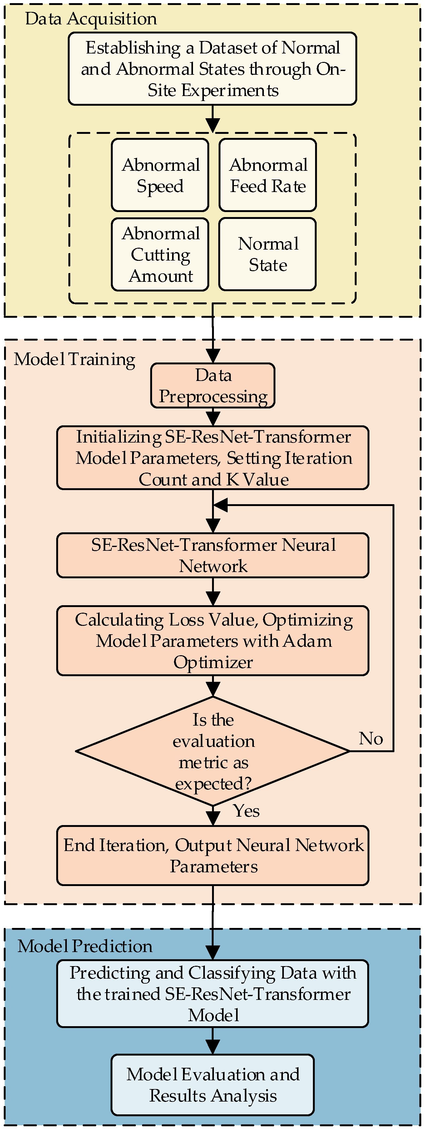
3.1. Data Acquisition

The comprehensive data on multiple sources of parameters, including current, operating temperature, and bearing vibration, comprehensively represent the operational status of CNC machine tools [29]. The SE-ResNet-Transformer model is trained using parameters derived from the CNC machine tool operating process. The model can predict typical operating states of the feed and spindle systems of the CNC machine tools, including the normal state, spindle speed abnormality, feed axis depth of cut abnormality, and feed volume abnormality. 
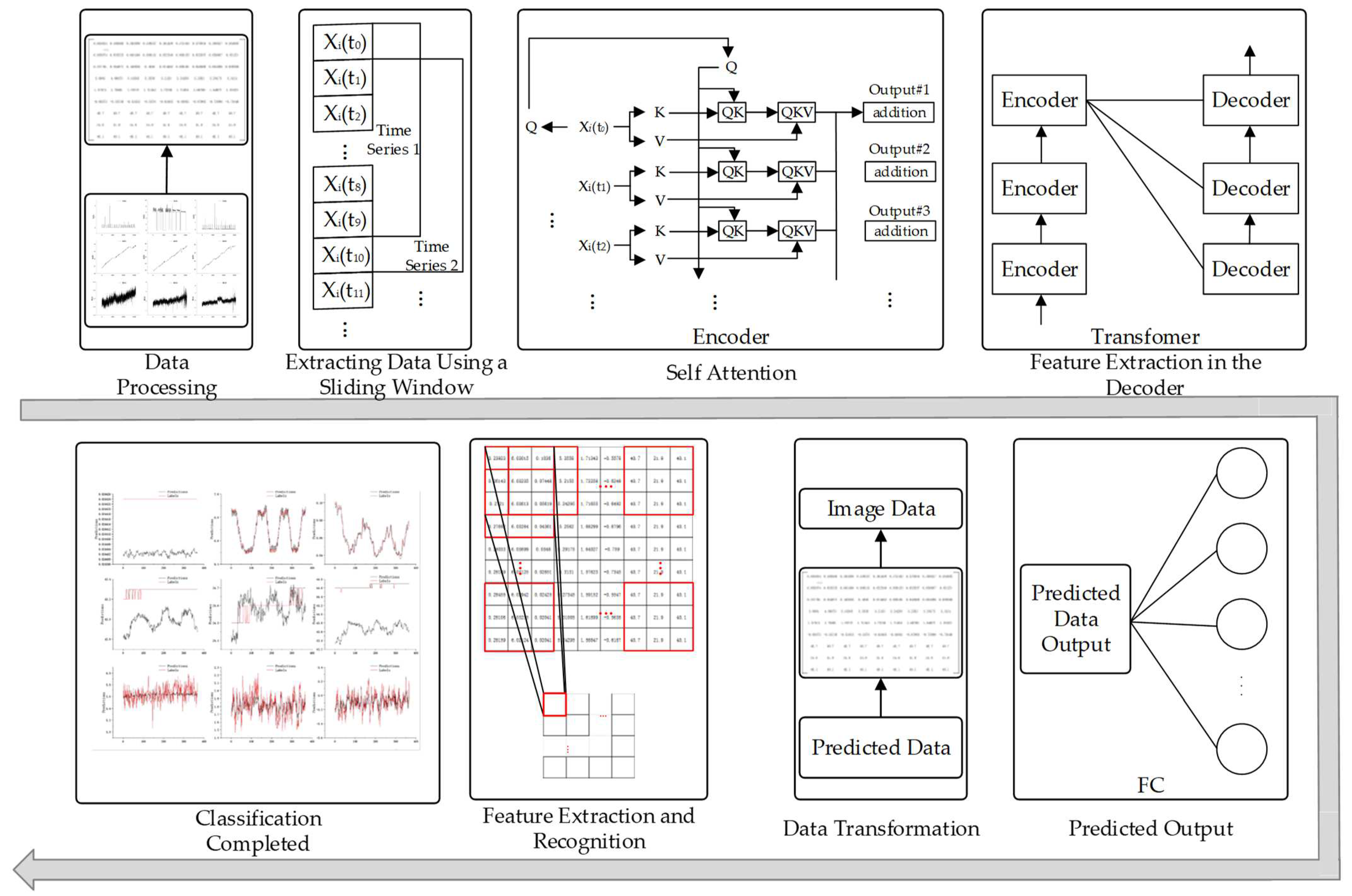
Figure 10 shows the input multi-source data and the output prediction states.
Data are collected on a CKA6150 CNC lathe (Dalian Machine Tool Group). The lathe is capable of simulating both normal and abnormal machining states. The temperatures of the lathe are collected using PT100-type temperature sensors, and the signals are transmitted through transmitters and preamplifiers to the data acquisition software. The currents are acquired using non-intrusive current sensors, and the signals are transmitted to the acquisition software via transmitters. Vibration data are obtained using acceleration sensors and transformed with a bespoke acquisition card. The data collections are synchronized through an Ethernet interface connected to the acquisition software. Figure 11 illustrates the sensor placement and sensor type.
Four CNC machine tool states are acquired, including normal state, abnormal spindle speed, abnormal depth of cut, and abnormal feed. The different states of the CNC machine are set by adjusting the cutting parameters of the CNC machine. Cutting parameters reflect temperature and current. Reportedly, the impact of tool wear on vibration and cutting parameters is small in the early and normal wear stages, but it is large in the severe wear stage [30]. The data used here are collected at the early wear and normal wear stages.
The data generated by the simulation for each state are presented in Table 2, and 60-mm diameter cast iron cylinders are used as simulation workpieces for machining. The parameters typically employed in the field of machining are established through the accumulation of relevant experience. Normal machining parameters are set based on machining experience. Abnormal spindle speed conditions encompass both excessively high and excessively low speeds, which impact surface quality and machining accuracy. During simulation of an abnormal state with increased depth of cut, the cutting force surges, and the spindle speed and feed remain unchanged. This situation leads to an increase in the vibration amplitude of the machined workpiece, thereby reducing the quality of the machined surface. However, surface quality is usually not affected when the depth of cut is reduced, so the only abnormal depth of cut occurs when the depth of cut is deepened. In the abnormal feed simulation, the feed rate is twice the normal feed rate, and the cutting force in this state is large, which is abnormal in the state of cutting a 60 mm cast iron cylinder. The surface quality is not degraded when the feed is reduced [31].
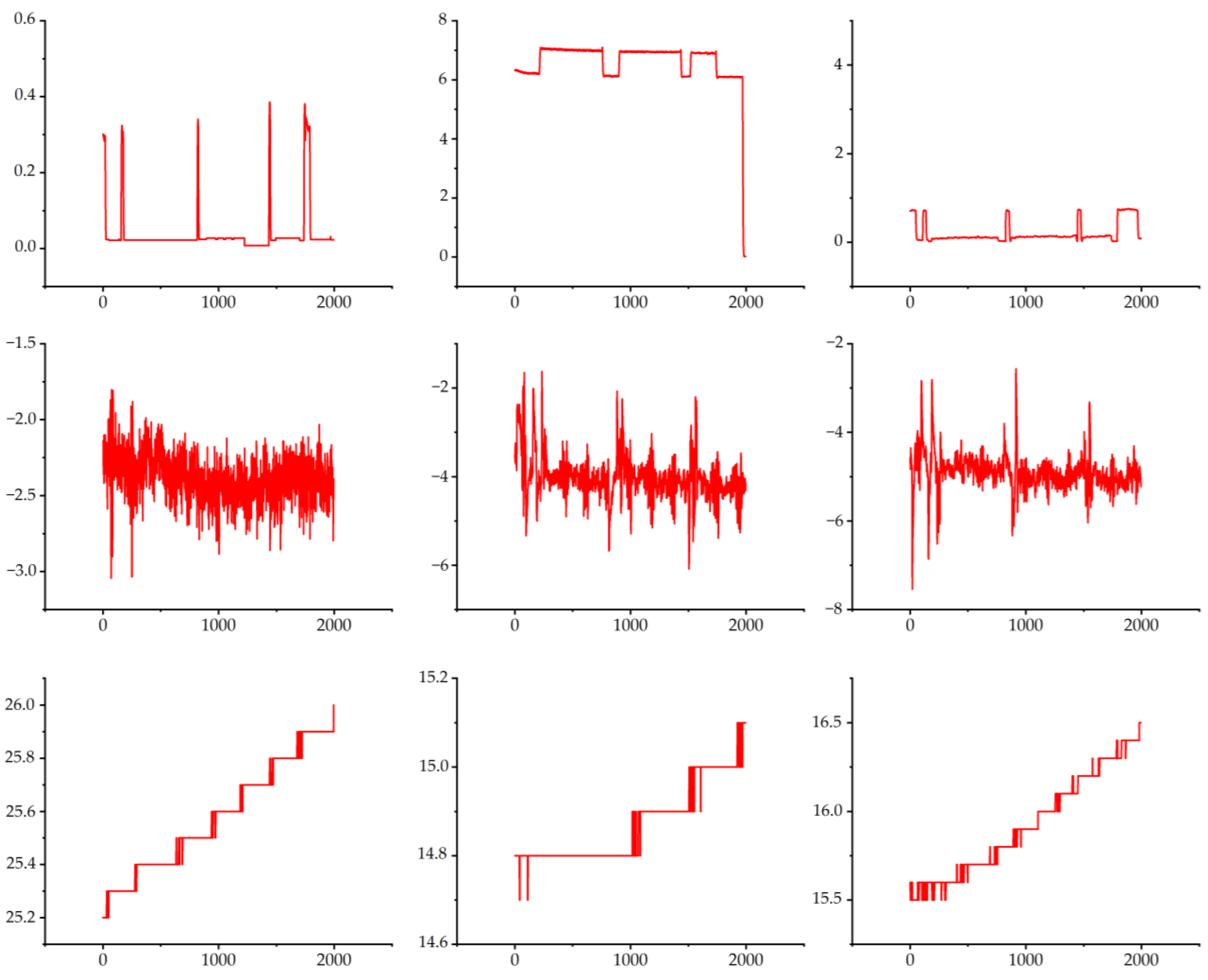
Figure 12 shows the 9 channels of data in the normal state after the data are processed to align the different channels with each other. In the machining process, the normal state is divided into three cycles, and a layer of cast iron is cut in each cycle. As the processing time is prolonged, the temperature slowly increases. The current data change periodically. During machining, the current data change accordingly when the machining process is switched. The vibration data show a high level of vibration during the process changeover. However, the vibration amplitude changes smoothly during machining.
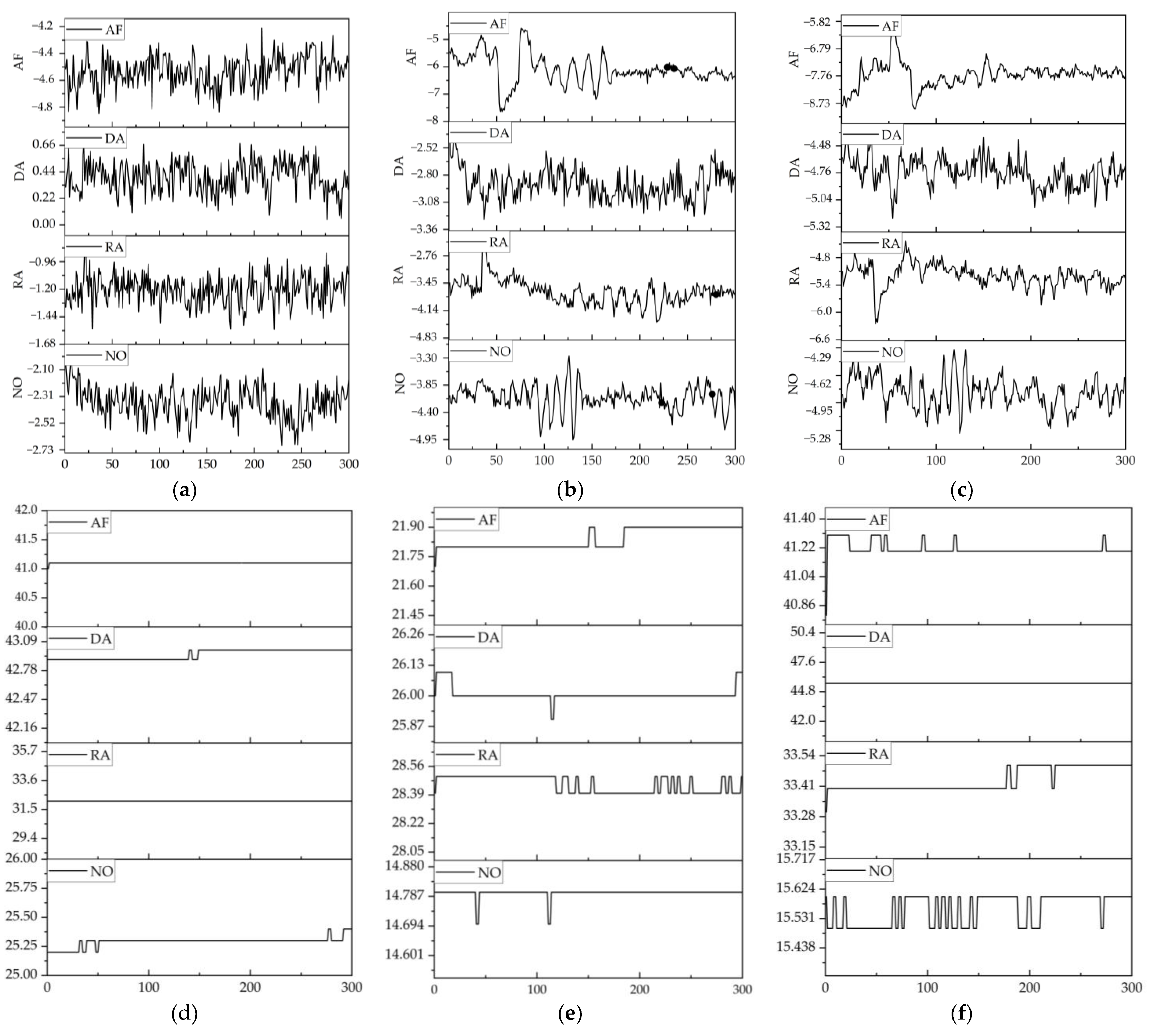
Figure 13 presents the time series of vibration and temperature under various states. Here, an analytical approach in the time domain is employed. Time series are collected, and the features embedded between the before and after time series are extracted. The extracted features are employed to investigate the information pertaining to the future time. The vibration data of a machine tool are used to illustrate the dynamic characteristics of the machine [32]. The amplitude of vibrations in different states exhibit a varying temporal profile (Figure 13). As reported, the vibration of CNC machine tools differs with different cutting parameters [29]. The vibration data are classified on the basis of the fact that different cutting parameters will demonstrate different trends when cutting. For the spindle vibration data, the range of amplitude in vibration differs among different states (cutting parameters) (Figure 13a). For example, the amplitude fluctuates around −2.3 in the normal state, but it fluctuates around −1.20, 0.4, and −4.6 in the RA, DA, and AF abnormal states, respectively (Figure 13a). The trends demonstrated in Figure 13b,c are different depending on the cutting parameters.
Characteristics of the different states are also embedded in the temperature data. Figure 13d–f shows the trends of the temperature data in different states. Clearly, the temperature of the same part differs among different states. In the case with an approximation of the temperature at the same part, the information of other parts can be used to make a judgement. When the temperature information is not enough, the state can be judged using diagnostic information and current information. Different states can be better judged through data fusion.

3.2. Experimental

The model is programmed and validated on a computer configured with i5-8300H, 8 G, and 1050 (Hewlett-Packard, Beijing, China), and the software integration environment is PyCharm (version PC-192.7142.42). About 70% of the data are utilized as a training set, 20% as a validation set, and 10% as a test set, based on the data collected above. The iteration number is absent, and training is deemed complete when the set threshold is met. The batch size is 32, and loss is evaluated using the mean square error (MSE) with the Adam optimization model. The parameters of this model are set in Table 3. The coefficient of determination (R2), mean absolute error (MAE), root mean square error (RMSE), and mean absolute percentage error (MAPE) [33] are used to evaluate the performance of the prediction method. A value of R2 closer to 1 indicates a better performance and more accurate prediction results. Values of MAE, RMSE, and MAPE closer to zero suggest that the predicted results are more accurate.

3.3. Experimental Results and Discussion

The model is trained, and the test set evaluation metrics are presented in Table 4. 
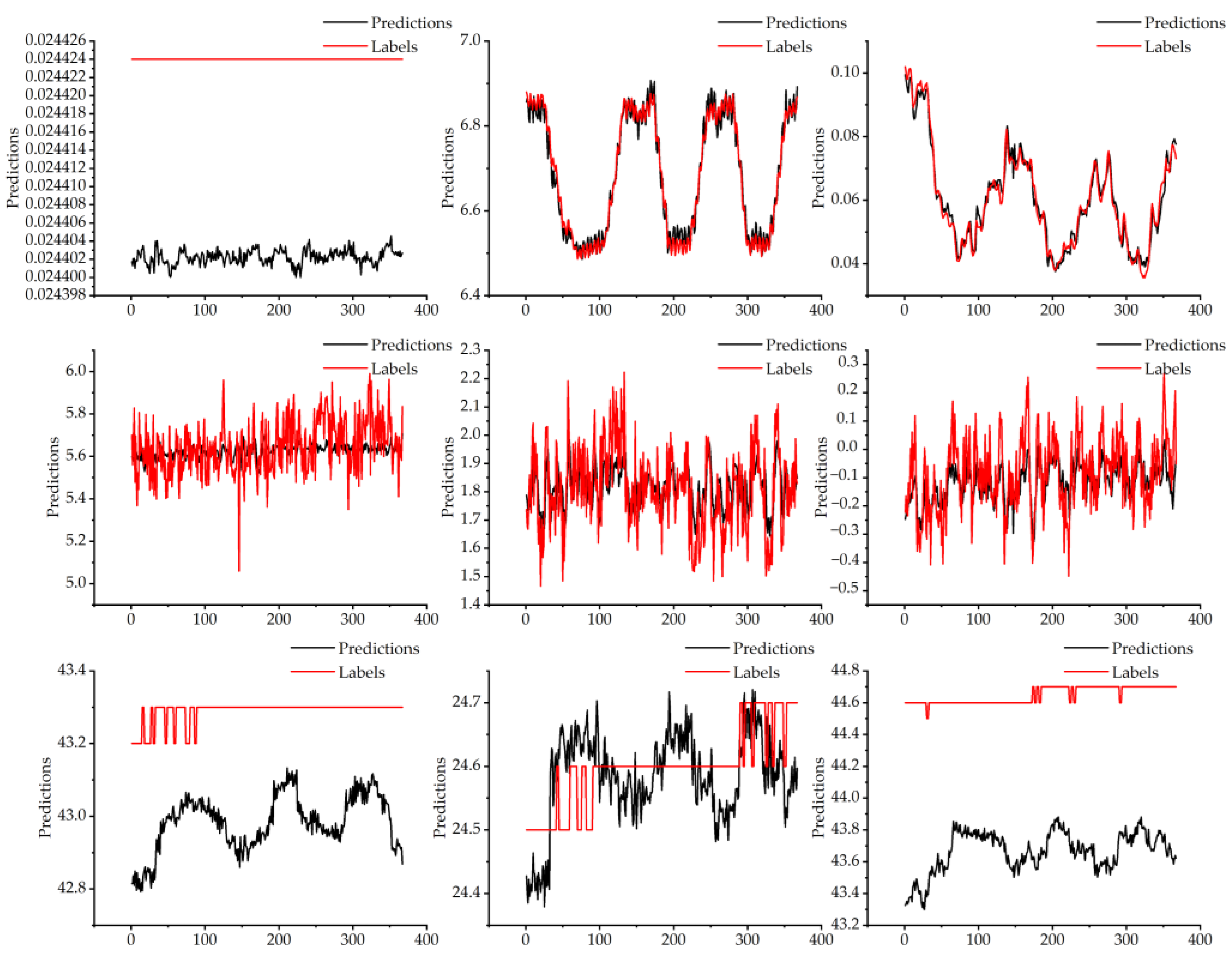
Figure 14 presents the results of the test set predictions. Table 4 and Figure 14 demonstrate a high degree of correlations among the spindle current, longitudinal feed axis, and vibration data. In other data, the value of R2 is not particularly high, but other indicators perform better. Among the data with a low value of R2, the detected value of the transverse incoming shaft current is 0.024424 A, and the predicted data vary around 0.024402. The three-axis temperature data change in a smooth trend. The range of variation in the given data is relatively limited, as the values vary by only 0.1°, 0.2°, and 0.2° over a total of 400 data points. R2 is calculated in a way that focuses only on the relationship between the mean and the predicted value. The data predicted by the model will increase errors and cause R2 to be inaccurate. However, when each datum is analyzed separately, the magnitude of change in the error range is not large and is within acceptable limits. The reason for this phenomenon is the inconsistency between the graduation value and accuracy of the input and output data. The data show that when the precision of the output data is higher than that of the real value, the evaluation effect is worse. In summary, the model is less sensitive to data with small magnitudes of change, insignificant trends, or small differences in input and output precision. Some of the data in the model are poorly evaluated, but with small errors, and thus can be used for feature recognition.
New evaluation metrics are incorporated to better describe the predictive performance of this model. The percentage of error between the predicted and true values can be expressed mathematically as follows:
X M = 1 i = 1 N y i ^     y i M N × 100 %
where M is the error, y i is the true value, and y i ^ is the predicted value,   y i ^ y i < 2 M .
The performance of the R2 underperformance data is evaluated (Table 5). Errors of the underperformance data are analyzed. The error between the true and predicted current in the transverse feed axis is within 0.000024. The difference between the two curves of predicted and actual data is large (Figure 12), but the error is small in actual usage. In prediction of temperature, the difference between each prediction and the true value is within 1, 0.3, and 1.4. In practice, the error is small and classification results are acceptable.
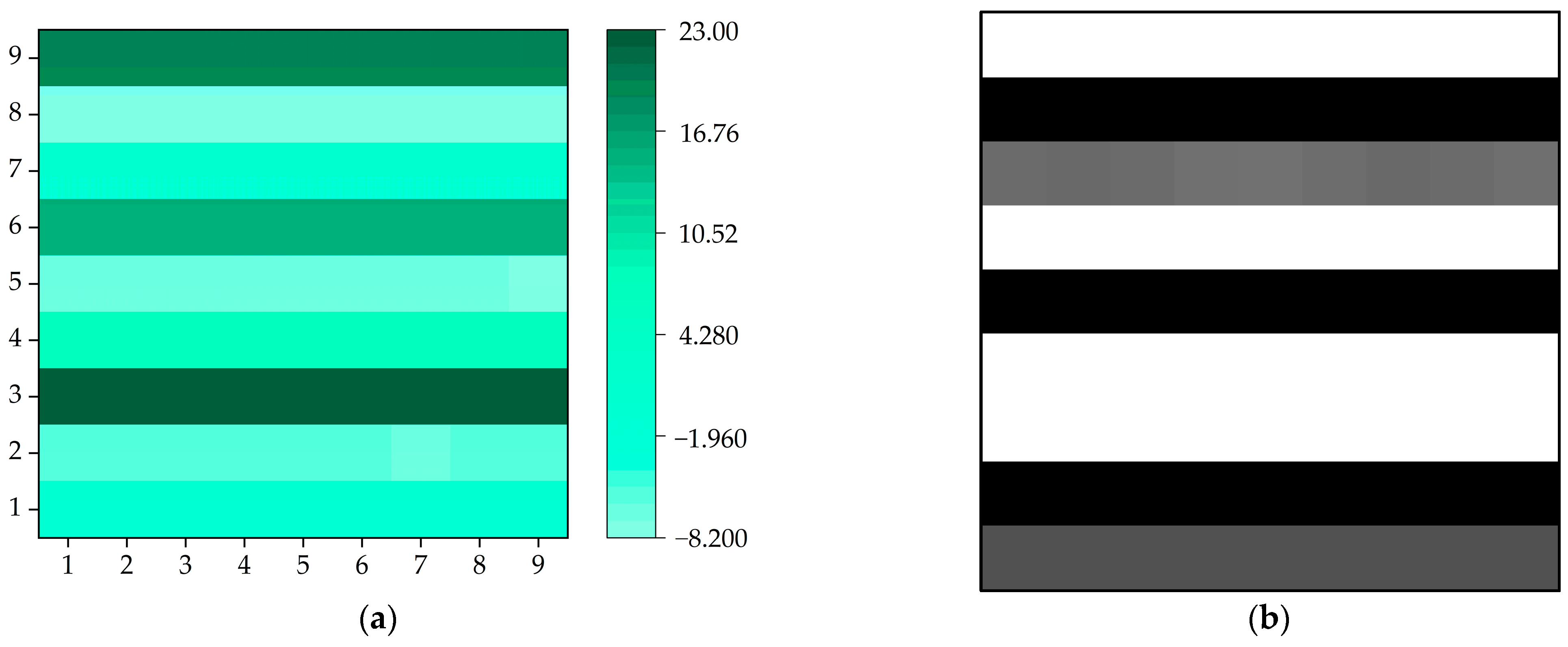
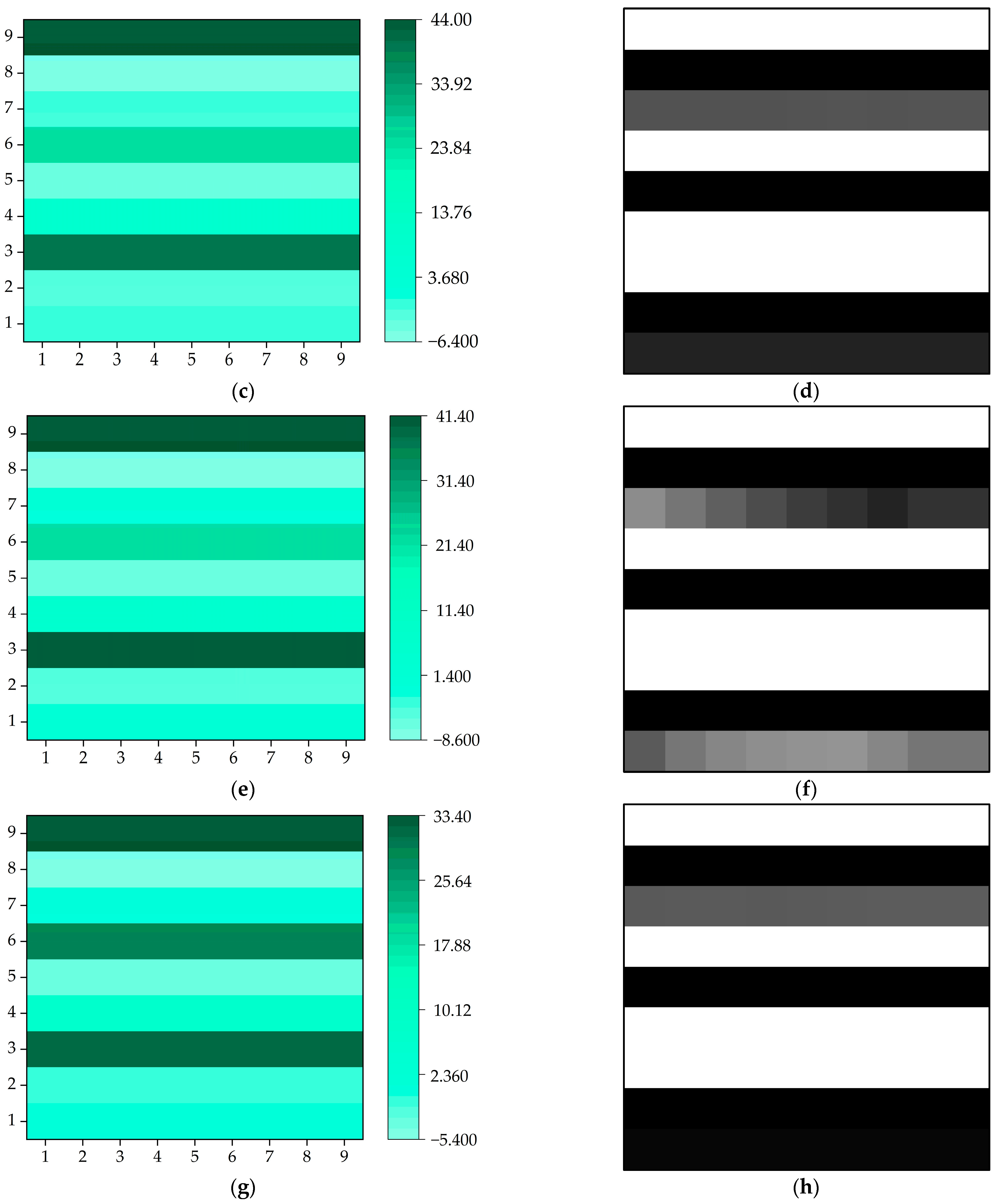
Once the prediction is completed, the predicted data are converted for image reconstruction, and the reconstructed image contains feature information. During the training, a sliding window is used to convert the data into a graph. The data from different channels differ in size among different states, and different data are shown in different colors in Figure 15. In Figure 15, there are two types of images, containing a visualization schematic and a real transformation image. Color images are transformed schematic images. Black-and-white images are real data images. This step successfully transforms the data classification situation into an image classification situation.
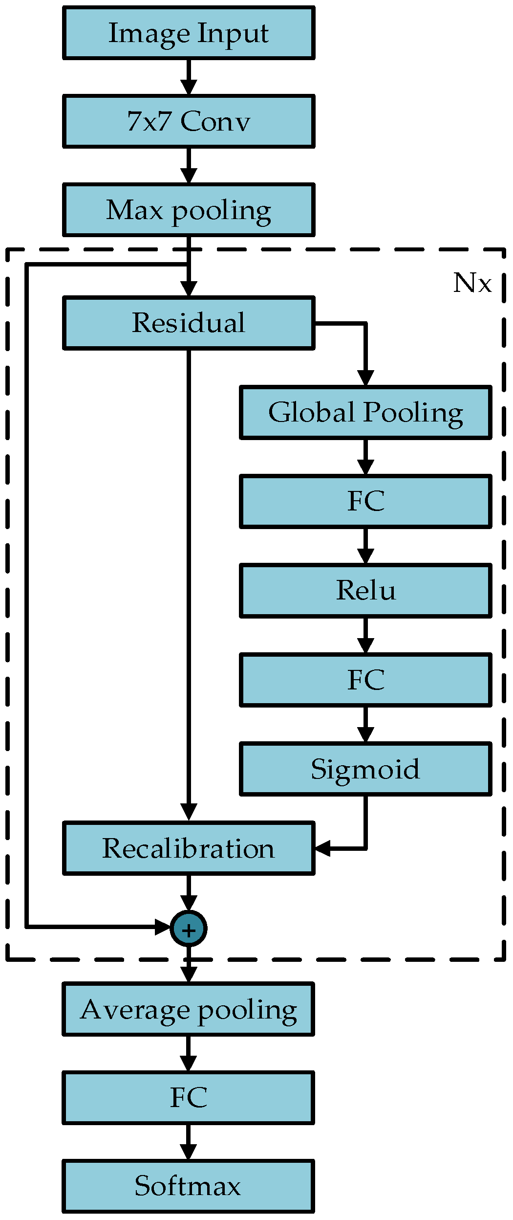
The input image in the SE-Resnet model is 9 × 9 in size, which is first converted to 32 × 32. The number of training data, number of classifications, batch size, learning rate, and weight decay coefficient are 50,000, 4, 128, 0.001, and 0.0005, respectively. The Adam optimization algorithm is used for updating. The evaluation metrics are accuracy and loss. Figure 16 shows the loss curve and accuracy curve with epochs. In the first three rounds of training, the loss rate on the training set sharply decreases, and the loss decreases severely, but still tends to be 0 on the validation set. This result indicates the model is converging and approaching 0. After 2 epochs, the accuracy on the test set is 100%, and the accuracy on the training set is 99.96% after an iteration to 10. After 5 epochs, the loss rates of the training and test sets are close to overlapping, and there is no excessive variation or overfitting in the curves. These results indicate the model is converging and approaching 0. The model can be trained only with 10 epochs. This is because an image in the format of 9 × 9 only contains 81 pieces of data. Moreover, this model achieves excellent results in 10 epochs of training, thanks to the better performance of the SE-Resnet model.
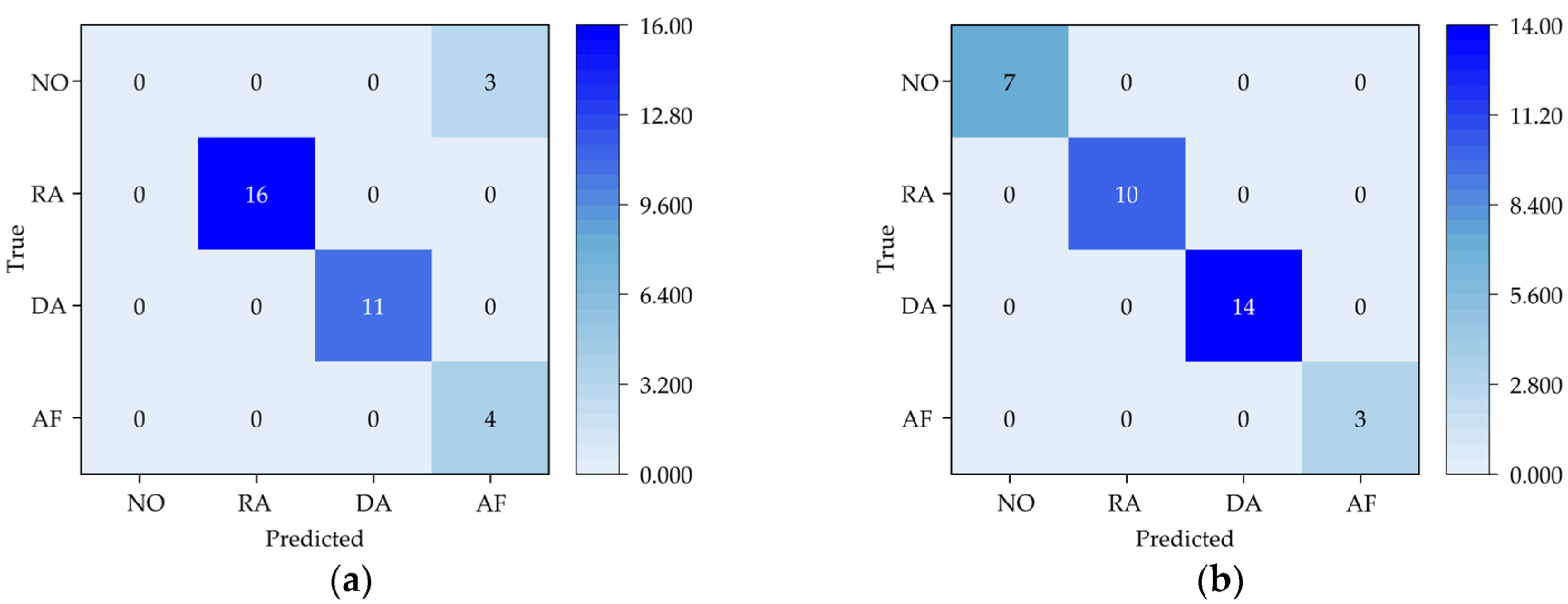
To better demonstrate the classification effect of the SE-Resnet model, a confusion matrix is used to show the classification on different epochs of the test set. NO, RA, DA, and AF in Figure 17 indicate normal state, abnormal speed, abnormal depth of cut, and abnormal feed, respectively. The confusion matrix consists of two axes representing the true labels and the classified labels, respectively. It discriminates the classification performance according to whether the data cluster is on the diagonal. When true and categorical labels match, they cluster on the diagonal. In cases of classification anomalies, the conditions under which the classification is made can be observed. In the first epoch, classification is evident on the validation set, but there are still cases of misclassification. Three sample points in the normal state are classified as feed anomalies, and the other three classification cases are accurate. In the second epoch of the accuracy surge, the classification on the validation set is excellent, and the four states can be perfectly classified to the states to which they belong.
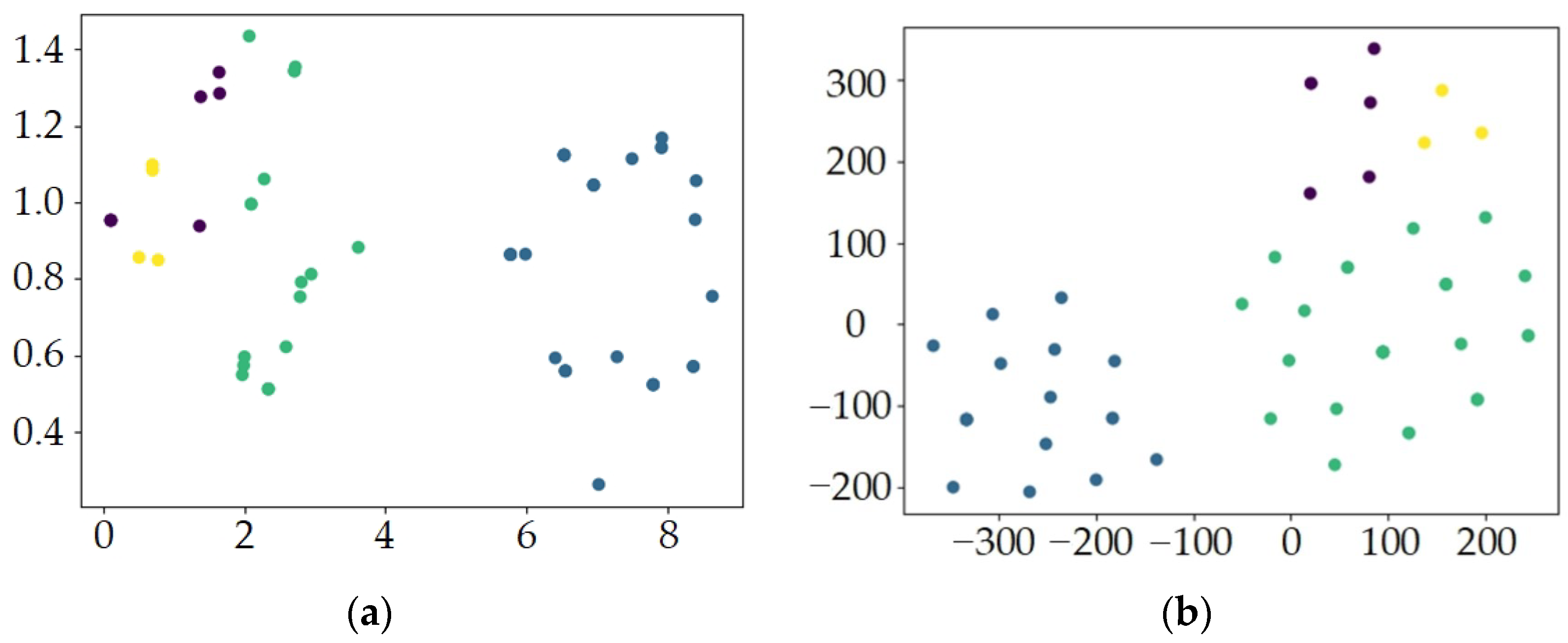
A non-linear dimensionality reduction method is used to validate the performance of the SE-Resnet network. A two-dimensional image is generated to represent the distribution of different categories within different epochs. The results shown in Figure 18 are from the two epochs, with a large difference in correctness between successive epochs, and the data are downscaled to a 2D plane. Poor clustering is shown in Figure 18, including high degrees of state mixing and state dispersion. In the case of high accuracy, the state separation is not obvious with fewer feature points, the other three state separation boundaries are clear, and clustering is effective. Although the clustering effect is different across different correctness conditions, it is not significant due to the difference in correctness at 3%.
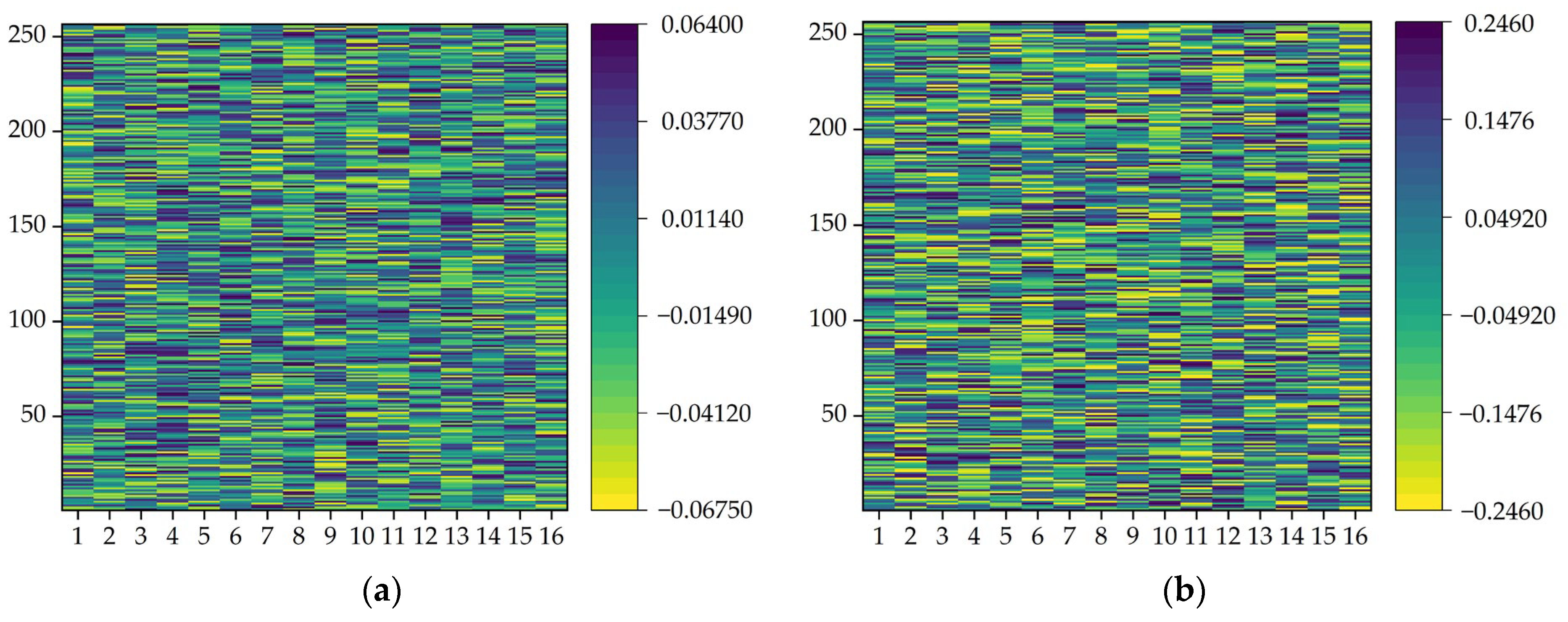
To further investigate the performance of the SE module in the SE-Resnet model, the attention matrices for different channels of the SE module are visualized after each round of training. Data from two channels of SE module attention are extracted from a single network and visualized in different state rounds according to the importance of non-canal data. Figure 19 shows the results after different visualizations of attention for the two modules in the same training session. The highest weight parameter in the second module is about 0.2 larger than that in the first module (0.06). This result indicates a significant channel in the second module. This significant channel has a weight parameter of 0.2 in the final result determination. The data in this channel are important and can be used in the prediction model to focus on increasing the prediction weights and better update the model performance.
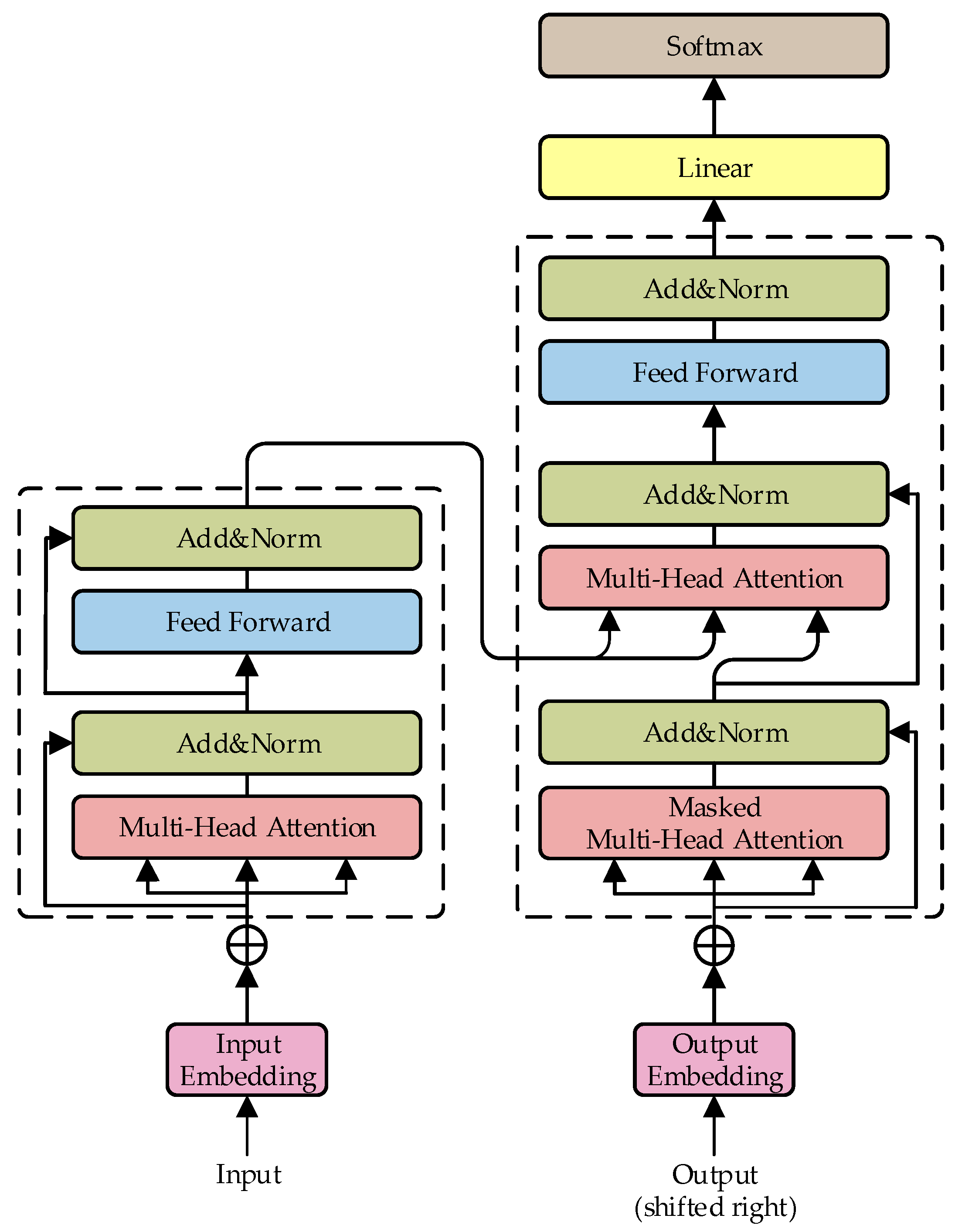
Experimental analysis is performed using the best model after training. The correctness of the method is verified against the predicted data labels. A known state is used as the input, and the current state is the label for the prediction. First, each of the four states is entered into the Transformer model, and thus four types of labeled predicted data are obtained. The four types of data are processed into 2D data, which are fed into the SE-Resnet model for classification. The accuracy of the classification is judged according to the classification results.
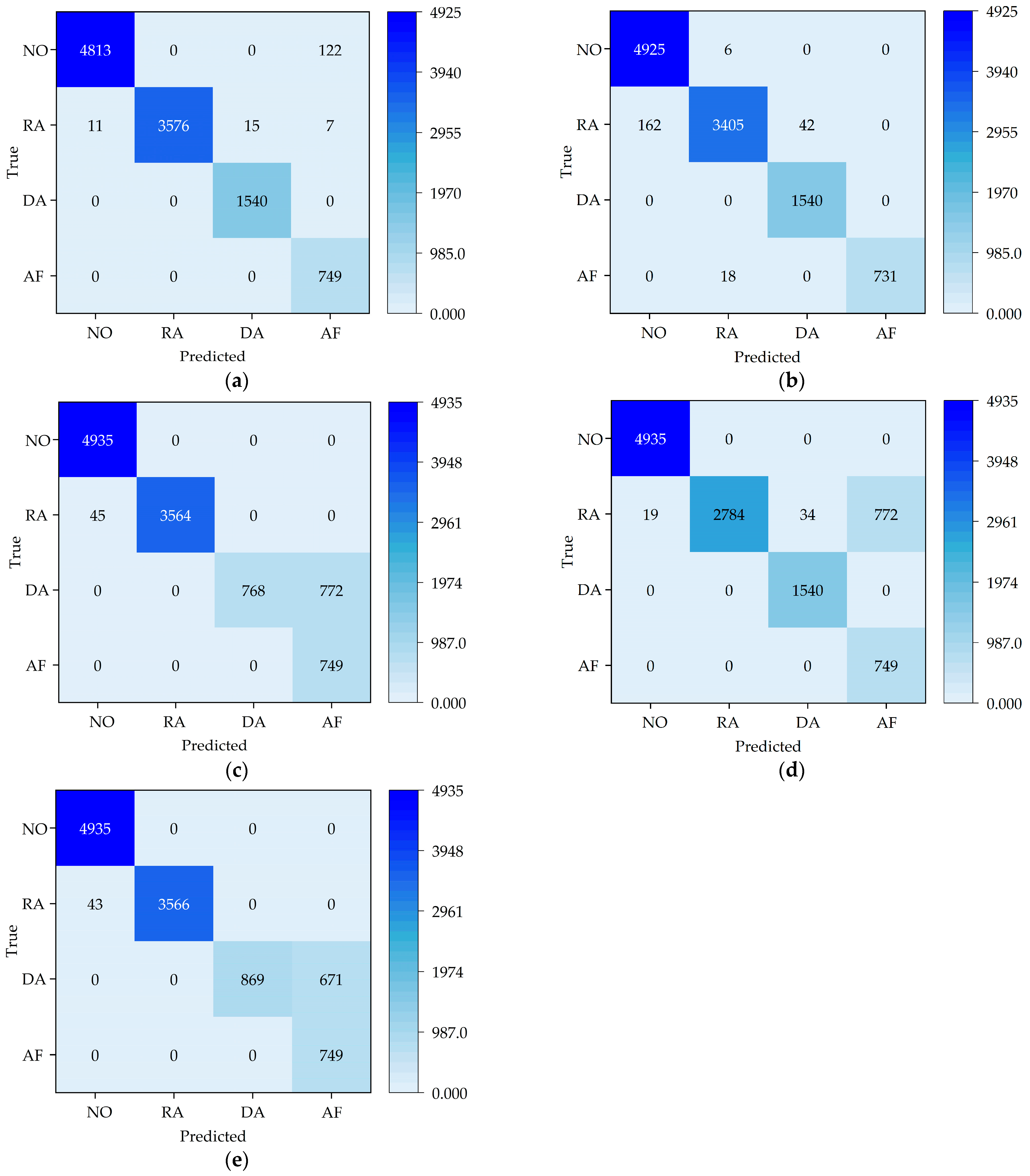
Figure 20 shows the confusion matrix plot of the predicted data displayed after classification. In Figure 20a, most of the normal state data are classified as normal, but 122 pieces of normal data are classified as abnormal. About 99% of the data in the RPM abnormal state are classified as normal, and 1% of the data are classified into the other three states. The feed rate is abnormal, and the depth-of-cut abnormal state is classified without error. The accuracy of this model is 98.56% (Table 6).
In the ResNet50 model, the correct rate is 0.67% lower compared to the network including the SE model. It is shown that the SE module improves the classification accuracy. The ResNet34 model has only 92.21% correct classification due to too few layers. The negative effects of too many layers can be eliminated by both the GooLeNet network and the ResNet model. Thus, the difference between the accuracy of the GoogLeNet network and the ResNet34 model is tiny: the accuracy of the GoogLeNet network is 92.45%; the accuracy of the AlexNet network is 93.41%.
The confusion matrix shows the classification error messages. The ResNet50 network is weak in resolving main spindle speed anomalies. The ResNet34 network is not able to distinguish the state of the depth-of-cut anomaly from the state of the feed anomaly. The AlexNet and ResNet34 networks are unable to distinguish the state of the depth-of-cut anomaly from the state of the feed anomaly. It is difficult to distinguish between main spindle speed anomalies and feed anomalies in the GoogLeNet network.

4. Conclusions

This study proposes a CNC machine tool failure prediction method based on SE-ResNet and Transformer. The method uses Transformer to extract temporal features from the acquired data and adopts the SE-ResNet model to extract spatial features. Then, the SE-ResNet-Transformer is obtained according to the two models. The SE-ResNet-Transformer extracts temporal and spatial features, predicts the data, and detects faults in CNC machine tools. In the extraction of spatial features, multi-channel data are combined. The data are transformed into a 2D matrix, and the different channel data are recalibrated in the SE module. This method is used to experiment on a dataset of nine channels and four categorical sets. It performs well and achieves a correct recognition rate of 98.56%. The method effectively improves the diagnostic performance, which is important for the safe detection and stable operation of CNC machine tools. Hence, this study provides a feasible method for accurately controlling the condition of CNC machine tools.

Author Contributions

Conceptualization, Z.W., L.H. and Y.J.; methodology, L.H.; software, W.W. and Q.G.; validation, Z.W., L.H. and Y.J.; data curation, W.W. and Q.G. All authors have read and agreed to the published version of the manuscript.

Funding

This research was funded by [the Basic Research Fund for State-owned Universities in Heilongjiang Province] grant number 145209404, [the Collaborative Education Project for Industry–University Cooperation Supported by the Ministry of Education] grant number 220602817220926, [the General Research Project on Higher-Education Teaching Reform in Heilongjiang Province] grant number SJGY20220410, [the Key Projects of Qiqihar City Scientific and Technological Plan] grant number ZDGG-202202, and [the Educational Science Research Project of Qiqihar University] grant number GJQTYB202212.

Data Availability Statement

All the data supporting the reported results have been included in this paper.

Conflicts of Interest

The authors declare no conflicts of interest.

References

  1. Zhang, X.; Guo, Q.; Liu, S.; Cheng, C. Analysis and Prospect of Deep Learning Technology and Its Fault Diagnosis Application. J. Xi’an Jiaotong Univ. 2020, 12, 54. [Google Scholar]
  2. Chen, H.; Zhong, K.; Ran, G.; Cheng, C. Deep Learning-Based Machinery Fault Diagnostics. Machines 2022, 10, 690. [Google Scholar] [CrossRef]
  3. Zhu, J.; Liu, T. Bidirectional Current WP and CBAR Neural Network Model-Based Bearing Fault Diagnosis. IEEE Access 2023, 11, 143635. [Google Scholar] [CrossRef]
  4. Hao, F.; Wang, H.; Li, H. Fault diagnosis of rollingbearingbased on continuous hidden Markov model. Chin. J. Constr. Mach. 2019, 2, 17. [Google Scholar] [CrossRef]
  5. Ahmed, H.O.A.; Nandi, A.K. Convolutional-Transformer Model with Long-Range Temporal Dependencies for Bearing Fault Diagnosis Using Vibration Signals. Machines 2023, 11, 746. [Google Scholar] [CrossRef]
  6. Qian, L.; Pan, Q.; Lv, Y.; Zhao, X. Fault Detection of Bearing by Resnet Classifier with Model-Based Data Augmentation. Machines 2022, 10, 521. [Google Scholar] [CrossRef]
  7. Afridi, Y.S.; Hasan, L.; Ullah, R.; Ahmad, Z.; Kim, J.-M. LSTM-Based Condition Monitoring and Fault Prognostics of Rolling Element Bearings Using Raw Vibrational Data. Machines 2023, 11, 531. [Google Scholar] [CrossRef]
  8. Ströbel, R.; Probst, Y.; Deucker, S.; Fleischer, J. Time Series Prediction for Energy Consumption of Computer Numerical Control Axes Using Hybrid Machine Learning Models. Machines 2023, 11, 1015. [Google Scholar] [CrossRef]
  9. Moysidis, D.A.; Karatzinis, G.D.; Boutalis, Y.S.; Karnavas, Y.L. A Study of Noise Effect in Electrical Machines Bearing Fault Detection and Diagnosis Considering Different Representative Feature Models. Machines 2023, 11, 1029. [Google Scholar] [CrossRef]
  10. Deng, F.; Chen, Z.; Liu, Y.; Yang, S.; Hao, R.; Lyu, L. A Novel Combination Neural Network Based on ConvLSTM-Transformer for Bearing Remaining Useful Life Prediction. Machines 2022, 10, 1226. [Google Scholar] [CrossRef]
  11. Sun, S.; Peng, T.; Huang, H. Machinery Prognostics and High-Dimensional Data Feature Extraction Based on a Transformer Self-Attention Transfer Network. Sensors 2023, 23, 9190. [Google Scholar] [CrossRef] [PubMed]
  12. Rama, V.S.B.; Hur, S.-H.; Yang, Z. Short-Term Fault Prediction of Wind Turbines Based on Integrated RNN-LSTM. IEEE Access 2024, 12, 22465. [Google Scholar] [CrossRef]
  13. Chen, X.; Chen, W.; Dinavahi, V.L.; Liu, Y.; Feng, J. Short-Term Load Forecasting and Associated Weather Variables Prediction Using ResNet-LSTM Based Deep Learning. IEEE Access 2023, 11, 5393. [Google Scholar] [CrossRef]
  14. Wanke, Y.; Chunhui, Z.; Biao, H. MoniNet with Concurrent Analytics of Temporal and Spatial Information for Fault Detection in Industrial Processes. IEEE Trans. Cybern. 2022, 52, 8. [Google Scholar] [CrossRef] [PubMed]
  15. Wanke, Y.; Chunhui, Z. Broad Convolutional Neural Network Based Industrial Process Fault Diagnosis with Incremental Learning Capability. IEEE Trans. Ind. Electron. 2020, 6, 67. [Google Scholar] [CrossRef]
  16. Wanke, Y.; Chunhui, Z. Robust Monitoring and Fault Isolation of Nonlinear Industrial Processes Using Denoising Autoencoder and Elastic Net. IEEE Trans. Control Syst. Technol. 2022, 28, 3. [Google Scholar] [CrossRef]
  17. Wang, L.; Zhang, C.; Zhu, J.; Xu, F. Fault Diagnosis of Motor Vibration Signals by Fusion of Spatiotemporal Features. Machines 2022, 10, 246. [Google Scholar] [CrossRef]
  18. Yu, Z.; Zhang, L.; Kim, J. The Performance Analysis of PSO-ResNet for the Fault Diagnosis of Vibration Signals Based on the Pipeline Robot. Sensors 2023, 23, 4289. [Google Scholar] [CrossRef]
  19. Lu, Q.; Chen, S.; Yin, L.; Ding, L. Pearson-ShuffleDarkNet37-SE-Fully Connected-Net for Fault Classification of the Electric System of Electric Vehicles. Appl. Sci. 2023, 13, 13141. [Google Scholar] [CrossRef]
  20. Quan, S.; Sun, M.; Zeng, X.; Wang, X.; Zhu, Z. Time Series Classification Based on Multi-Dimensional Feature Fusion. IEEE Access 2023, 11, 11066. [Google Scholar] [CrossRef]
  21. Hongfeng, G.; Jie, M.; Zhonghang, Z.; Chaozhi, C. Bearing Fault Diagnosis Method Based on Attention Mechanism and Multi-Channel Feature Fusion. IEEE Access 2024, 12, 45011. [Google Scholar] [CrossRef]
  22. Fu, Y.; Chen, X.; Liu, Y.; Son, C.; Yang, Y. Gearbox Fault Diagnosis Based on Multi-Sensor and Multi-Channel Decision-Level Fusion Based on SDP. Appl. Sci. 2022, 12, 7535. [Google Scholar] [CrossRef]
  23. Liu, Y.; Xiang, H.; Jiang, Z.; Xiang, J. A Domain Adaption ResNet Model to Detect Faults in Roller Bearings Using Vibro-Acoustic Data. Sensors 2023, 23, 3068. [Google Scholar] [CrossRef]
  24. Zhu, J.; Zhao, Z.; Zheng, X.; An, Z.; Guo, Q.; Li, Z.; Sun, J.; Guo, Y. Time-Series Power Forecasting for Wind and Solar Energy Based on the SL-Transformer. Energies 2023, 16, 7610. [Google Scholar] [CrossRef]
  25. Chen, T.; Qin, H.; Li, X.; Wan, W.; Yan, W. A Non-Intrusive Load Monitoring Method Based on Feature Fusion and SE-ResNet. Electronics 2023, 12, 1909. [Google Scholar] [CrossRef]
  26. Shaheed, K.; Qureshi, I.; Abbas, F.; Jabbar, S.; Abbas, Q.; Ahmad, H.; Sajid, M.Z. EfficientRMT-Net—An Efficient ResNet-50 and Vision Transformers Approach for Classifying Potato Plant Leaf Diseases. Sensors 2023, 23, 9516. [Google Scholar] [CrossRef] [PubMed]
  27. Wang, N.; Zhao, X. Time Series Forecasting Based on Convolution Transformer. IEICE Trans. Inf. Syst. 2023, 5, 976. [Google Scholar] [CrossRef]
  28. Fei, M.; Zhijie, Y.; Jiangbo, W.; Qipeng, S.; Bo, B.; Qingyuan, G.; Kai, H. Short-term traffic flow velocity prediction method based on multi-channel fusion of meteorological and transportation data. J. Traffic Transp. Eng. 2024, 1, 17. Available online: http://kns.cnki.net/kcms/detail/61.1369.U.20240418.1116.002.html (accessed on 14 April 2024).
  29. Chungwen, M.; Jiangming, D.; Yuzheng, C.; Huaiyuan, L.; Zhicheng, S.; Jing, X. The relationships between cutting parameters, tool wear, cutting force and vibration. Adv. Mech. Eng. 2018, 10, 1. [Google Scholar] [CrossRef]
  30. Owais Qadri, M.; Namazi, H. Fractal-based analysis of the relation between tool wear and machine vibration in milling operation. Fractals 2022, 28, 6. [Google Scholar] [CrossRef]
  31. Fan, C.; Chen, H.; Kuo, T. Prediction of machining accuracy degradation of machine tools. Precis. Eng. 2012, 2, 288. [Google Scholar] [CrossRef]
  32. Li, C.; Song, Z.; Huang, X.; Zhao, H.; Jiang, X.; Mao, X. Analysis of Dynamic Characteristics for Machine Tools Based on Dynamic Stiffness Sensitivity. Processes 2021, 9, 2260. [Google Scholar] [CrossRef]
  33. Chen, C.; Qiu, A.; Chen, H.; Chen, Y.; Liu, X.; Li, D. Prediction of Pollutant Concentration Based on Spatial–Temporal Attention, ResNet and ConvLSTM. Sensors 2023, 23, 8863. [Google Scholar] [CrossRef] [PubMed]
Figure 1. Structure of SE-ResNet-Transformer.
Machines 12 00418 g001
Figure 2. Fault prediction flowchart of the proposed fault prediction method.
Machines 12 00418 g002
Figure 3. Computational principle of squeeze-and-excitation.
Machines 12 00418 g003
Figure 4. Residual structure diagram: (a) CNN normal block; (b) CNN residual block.
Machines 12 00418 g004
Figure 5. Architecture of SE-ResNet.
Machines 12 00418 g005
Figure 6. Structure of Transformer.
Machines 12 00418 g006
Figure 7. Schematic representation of multi-head attention.
Machines 12 00418 g007
Figure 8. Mode of data fusion.
Machines 12 00418 g008
Figure 9. Workflow of SE-ResNet-Transformer model.
Machines 12 00418 g009
Figure 10. Input data and predicted states.
Machines 12 00418 g010
Figure 11. Data collection site and sensor layout.
Machines 12 00418 g011
Figure 12. Collected data.
Machines 12 00418 g012
Figure 13. Collected data of vibration and temperature: (a) spindle vibration, (b) cross-feed axis vibration, (c) longitudinal feed axis vibration, (d) main motor temperature, (e) cross-feed axis temperature, (f) longitudinal feed axis temperature.
Machines 12 00418 g013
Figure 14. Comparison of real and projected data.
Machines 12 00418 g014
Figure 15. Two-dimensional data visualization: (a,b) normal state; abnormal states, (c,d) cutting depth, (e,f) feed rate, (g,h) main spindle speed.
Machines 12 00418 g015aMachines 12 00418 g015b
Figure 16. Loss and correctness in classification models: (a) loss; (b) accuracy.
Machines 12 00418 g016
Figure 17. Classification confusion matrix during training: (a) first epoch; (b) second epoch.
Machines 12 00418 g017
Figure 18. Two-dimensional scatter clustering: (a) first epoch; (b) second epoch.
Machines 12 00418 g018
Figure 19. Attention visualization for different modules in the same epoch: (a) first module; (b) second module.
Machines 12 00418 g019
Figure 20. Confusion matrix for 5 models: (a) SE-ResNet, (b) ResNet50, (c) ResNet34, (d) GoogLeNet, (e) AlexNet.
Machines 12 00418 g020
Table 1. Architecture of SE-ResNet50.
Layer NameOutput Size50-Layer
Conv1 112 × 1127 × 7, 64, stride2
Conv2_x56 × 563 × 3, max pool, stride2
1 × 1,64 3 × 3.64 1 × 1 ,   256 f c , 16 , 256 × 3
Conv3_x28 × 28 1 × 1 ,   128 3 × 3 ,   128 1 × 1 ,   512 f c , 32 , 512 × 4
Conv4_x14 × 14 1 × 1 ,   256 3 × 3 ,   256 1 × 1 ,   1024 f c , 64 , 1024 × 6
Conv5_x7 × 7 1 × 1 ,   512 3 × 3 ,   512 1 × 1 ,   2048 f c , 128 , 2048 × 3
1 × 1Average pool, 1000-d fc, softmax
FLOPs3.8 × 109
Table 2. Parameters of different simulation states of CNC machine tools.
CNC Machine StatusSpindle Speed (r/min)Feed Rate (mm/r)Depth of Cut (mm)
Normal state 5000.21
Abnormal spindle speed2000.21
10000.21
Abnormal depth of cut5000.22
Abnormal feed5000.41
Table 3. Model parameters.
ParametersValue
Initial learning rate0.001
Activation functionReLU
OptimizerAdam
Number of heads4
Hidden size64
Table 4. Evaluation indicators for each parameter of machine tools during training.
Parameters of Machine ToolsR2MAERMSEMAPE
Main motor current0.9370.01840.0230.027
Cross-feed axis motor current06.05 × 10−56.74 × 10−50.0029
Longitudinal feed axis motor current0.97090.00220.00260.0383
Spindle vibration0.04210.09980.12470.176
Cross-feed axis vibration0.28630.09760.12160.0543
Longitudinal feed axis vibration0.30420.08740.107934.0182
Main motor temperature−97.45530.30470.31250.007
Cross-feed axis temperature0.57840.0630.07550.0025
Longitudinal feed axis temperature−366.7640.98180.98910.0219
Table 5. Percentage of error in data of machine tools.
Error LevelCross-Feed Axis Motor CurrentMain Motor Temperature Cross-Feed Axis TemperatureLongitudinal Feed Axis Temperature
0.000021.36%---
0.00002150.40%---
0.00002261.30%---
0.00002394.84%---
0.000024100%-0-
0.003--55.84%-
0.1-080.38%-
0.15-0.81%96.73%-
0.3-44.41%100%-
0.3047-69.75%--
0.4-94.27%--
0.5-99.72%-0
1-100%-54.22%
1.1---83.10%
1.2---95.36%
1.3---99.72%
1.4---100%
Table 6. Correctness of the 5 models.
MethodSE-ResNetResNet50ResNet34GoogLeNetAlexNet
Accuracy (%)98.5697.8992.2192.4593.41
Disclaimer/Publisher’s Note: The statements, opinions and data contained in all publications are solely those of the individual author(s) and contributor(s) and not of MDPI and/or the editor(s). MDPI and/or the editor(s) disclaim responsibility for any injury to people or property resulting from any ideas, methods, instructions or products referred to in the content.

