


A Fault Prediction Method for CNC Machine Tools Based on SE-ResNet-Transformer
Abstract
:1. Introduction
- 1.
- In this study, the Transformer model and SE-ResNet model are used jointly. The state classification module was added after the data prediction module to efficiently and accurately complete the classification of predicted fault data.
- 2.
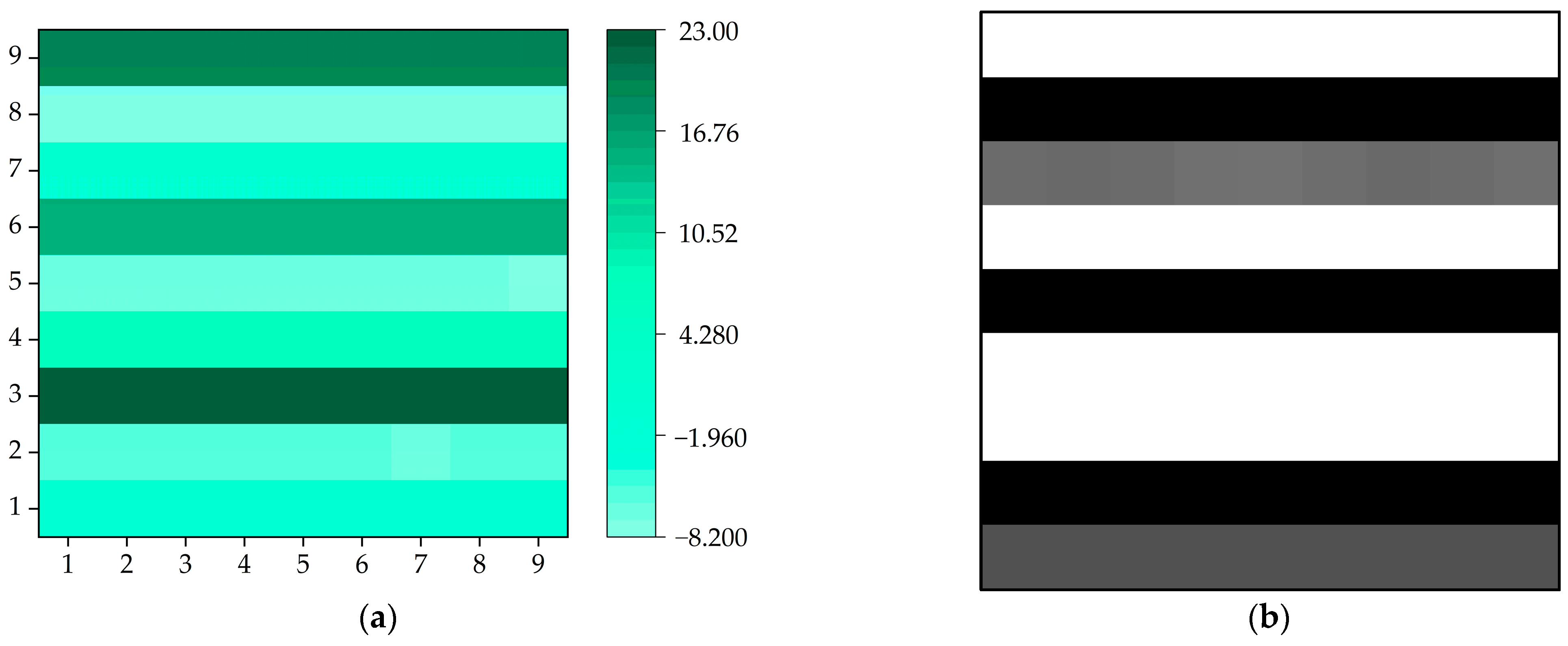
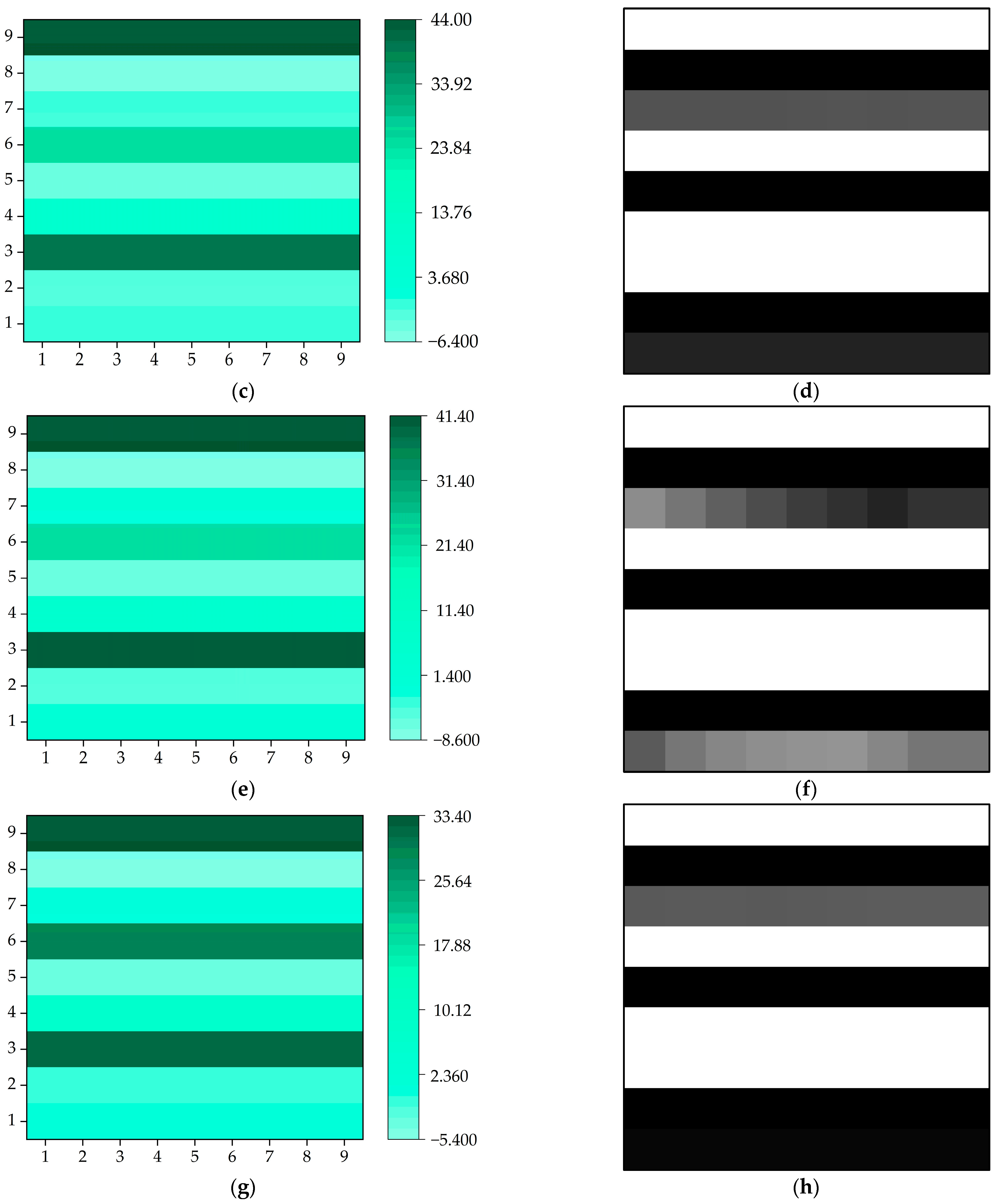
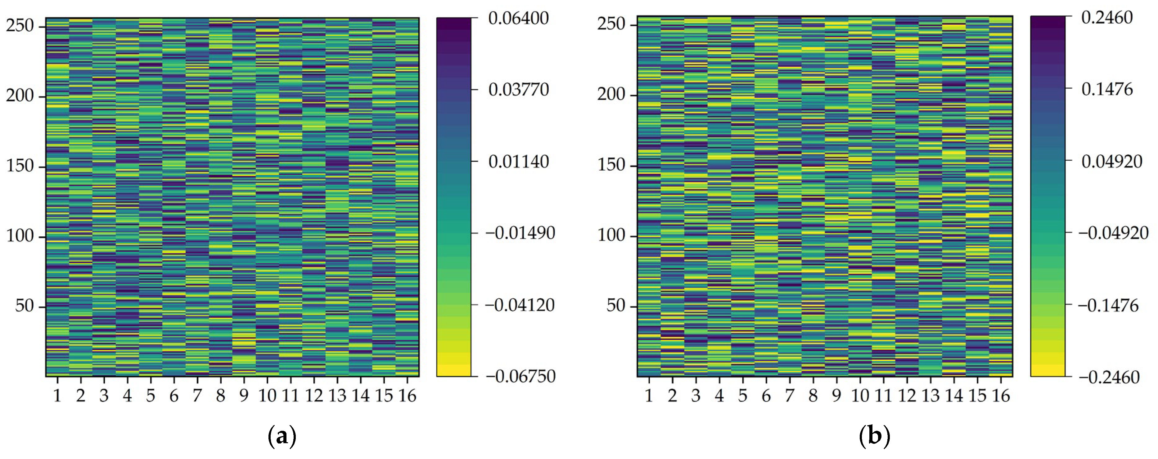
- The spatial connections between different predicted feature data are improved through two-dimensional data fusion. The data fusion module combines the independent data. This approach allows not only temporal but also spatial features to be extracted during the convolution operation. This transforming enables cross-data feature extraction and recognition, thereby strengthening the identification capability of this method.
- 3.
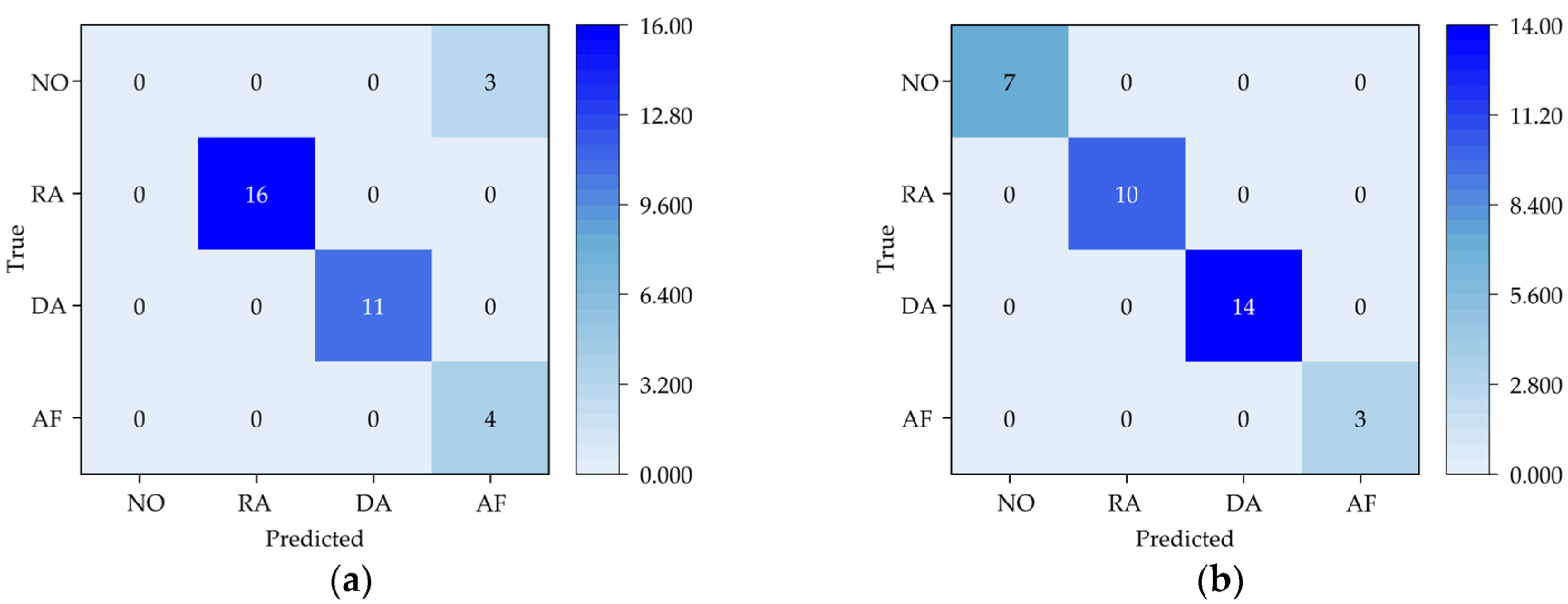
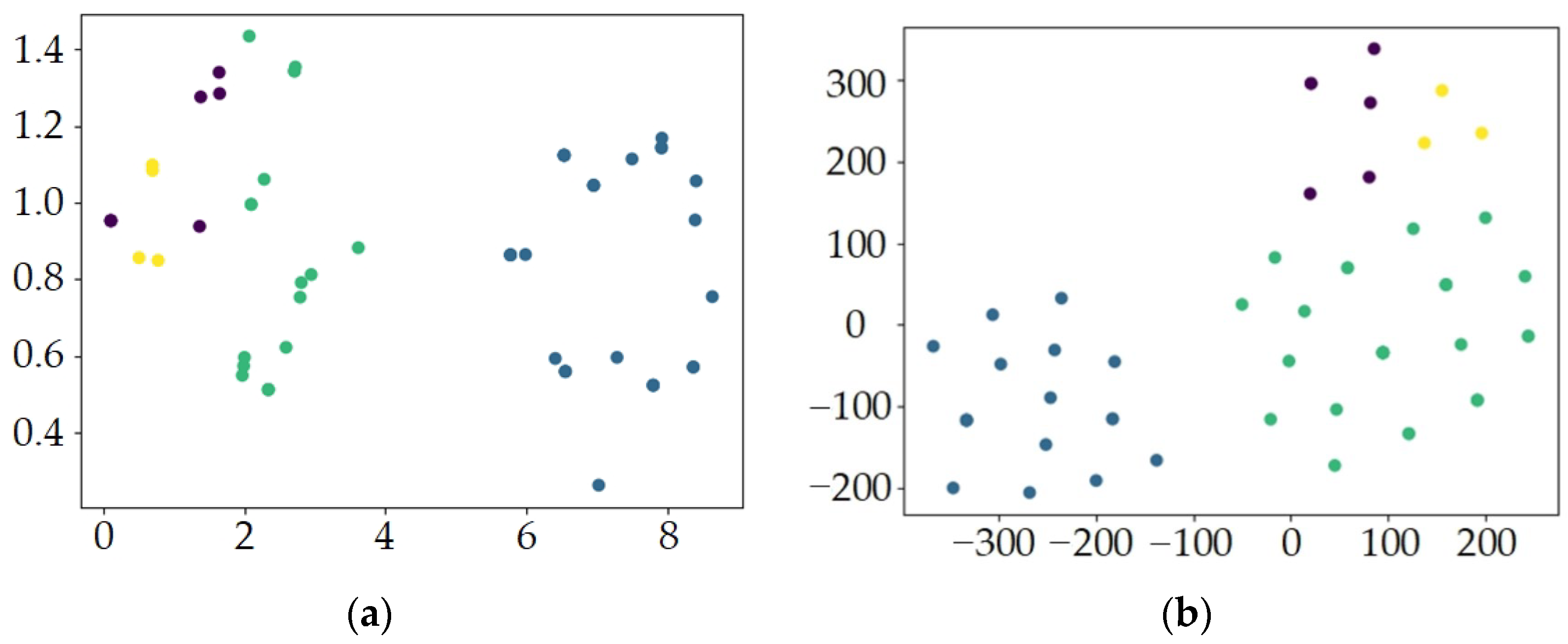
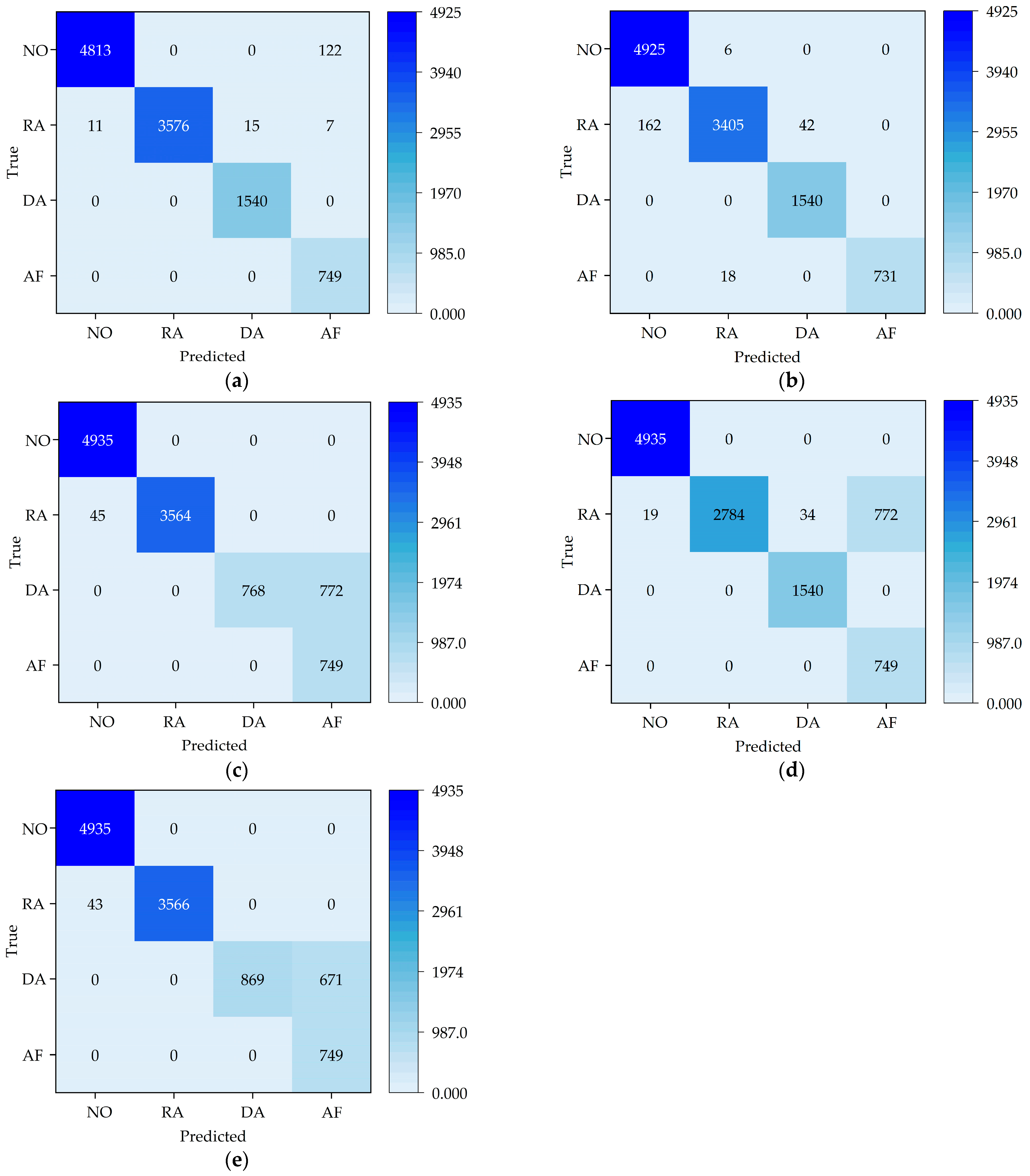
- A dataset is established by simulating different states of CNC machine tools through experimental simulations. The proposed method is experimentally validated on the dataset, achieving a prediction accuracy of 98.56%. The effectiveness of the proposed method is thus validated.
2. The Proposed Method
2.1. SE-ResNet-Transformer Model
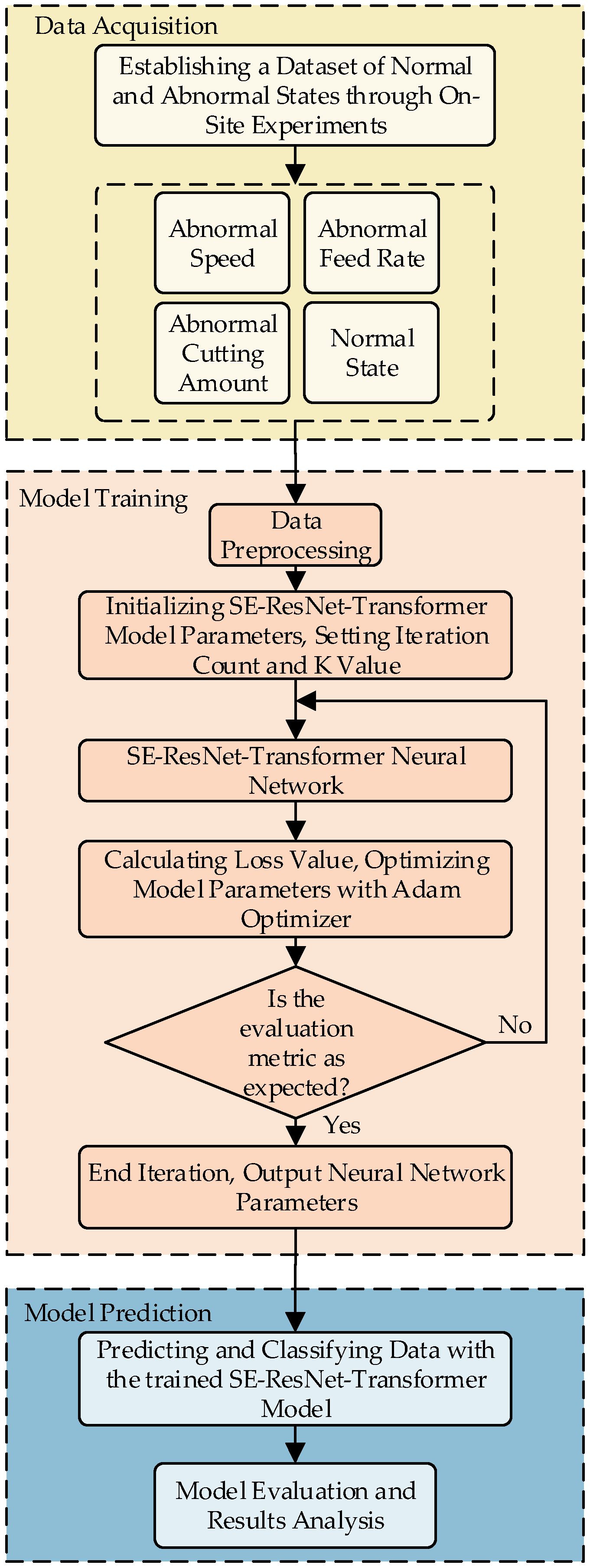
- (1)
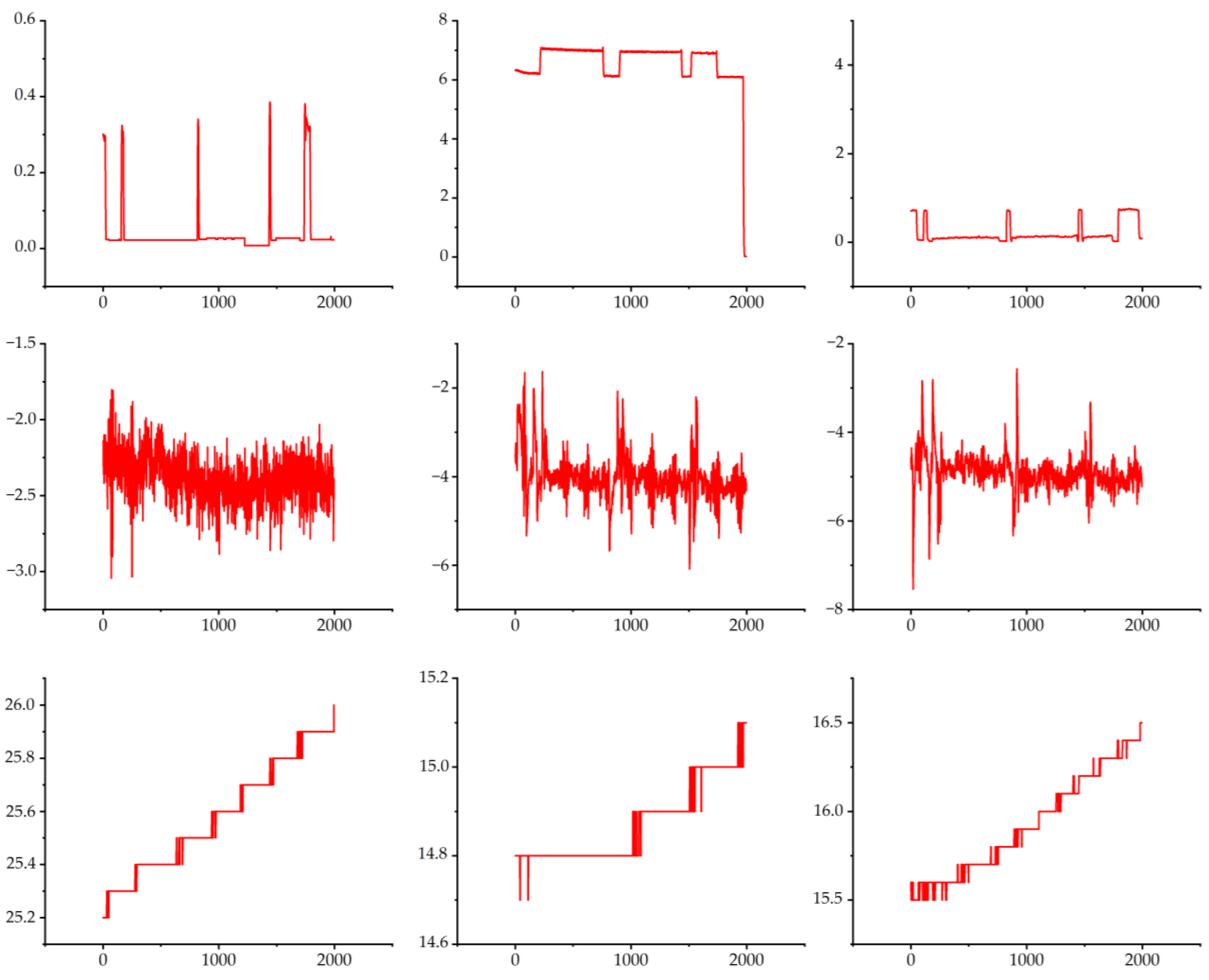
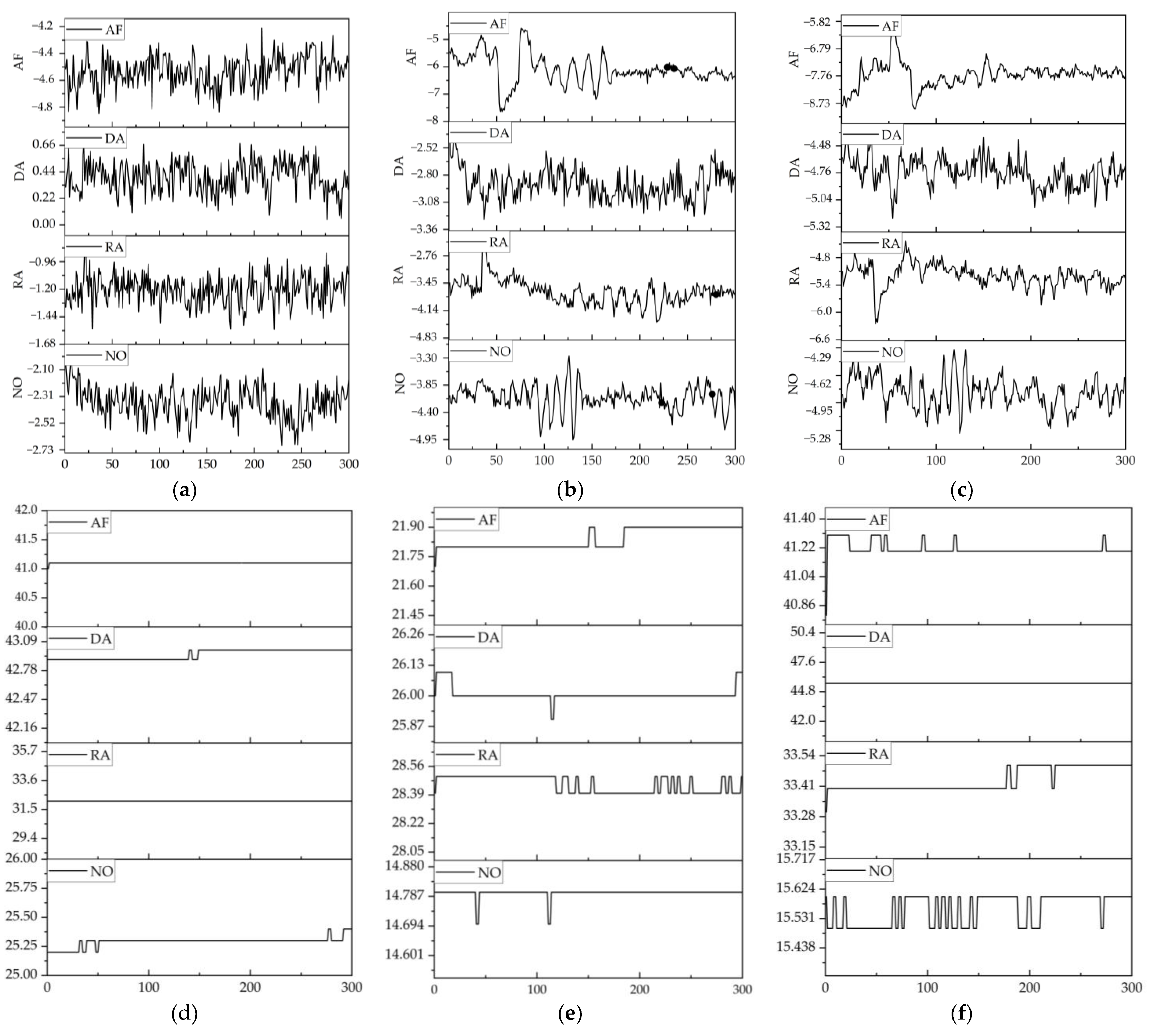
- On-site experiments are conducted, where workpieces are processed to simulate four states, including a normal condition and three abnormal conditions. As a result, four scenarios and data from nine channels are generated and used to construct a CNC machine tool status dataset. The dataset is randomly partitioned into training and testing sets.
- (2)
- After data collection, the data are preprocessed to integrate data trend transformations, enabling the extraction of data trends under different states.
- (3)
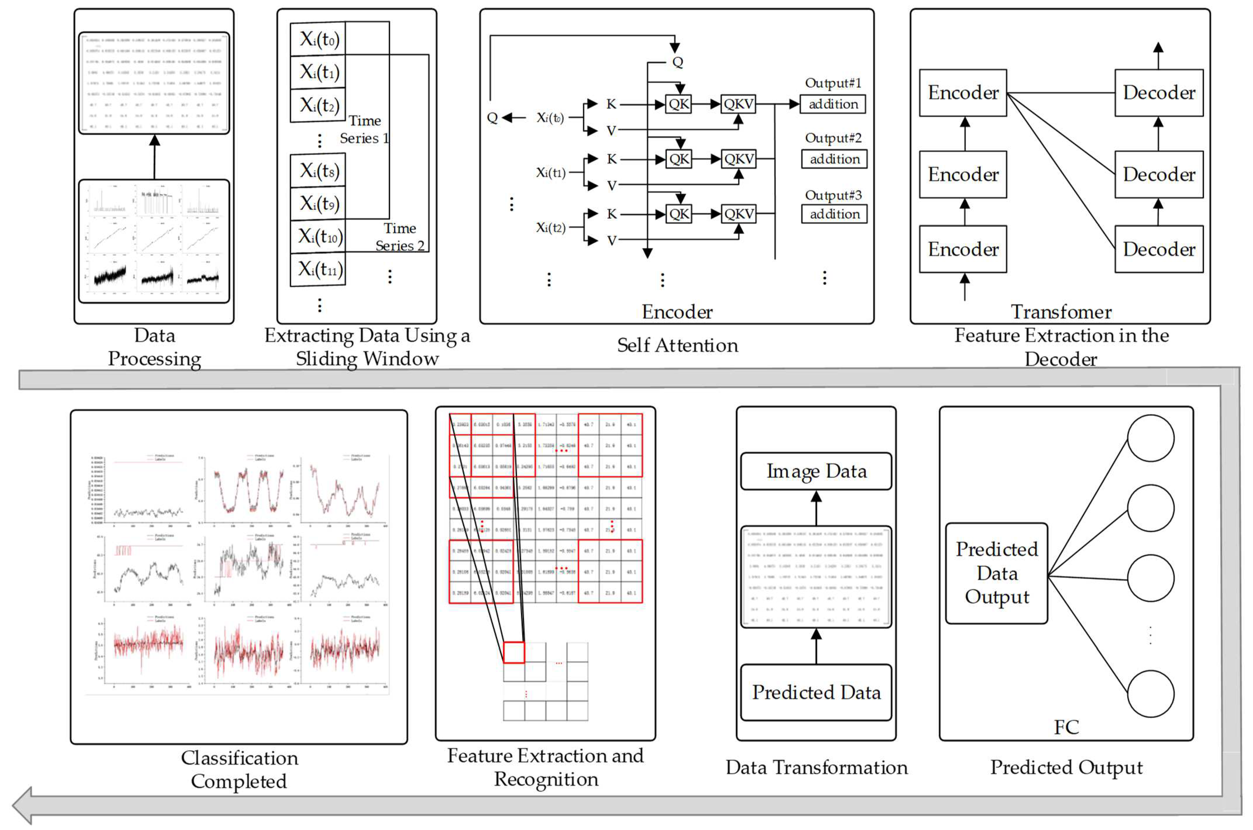
- An SE-ResNet-Transformer model is established and trained using the training set. The CNC machine tool status data are used as the input to the SE-ResNet-Transformer model, and the predicted CNC machine tool status is the output. The data are processed through an encoder-decoder, and a classifier is employed to identify specific operating states.
- (4)
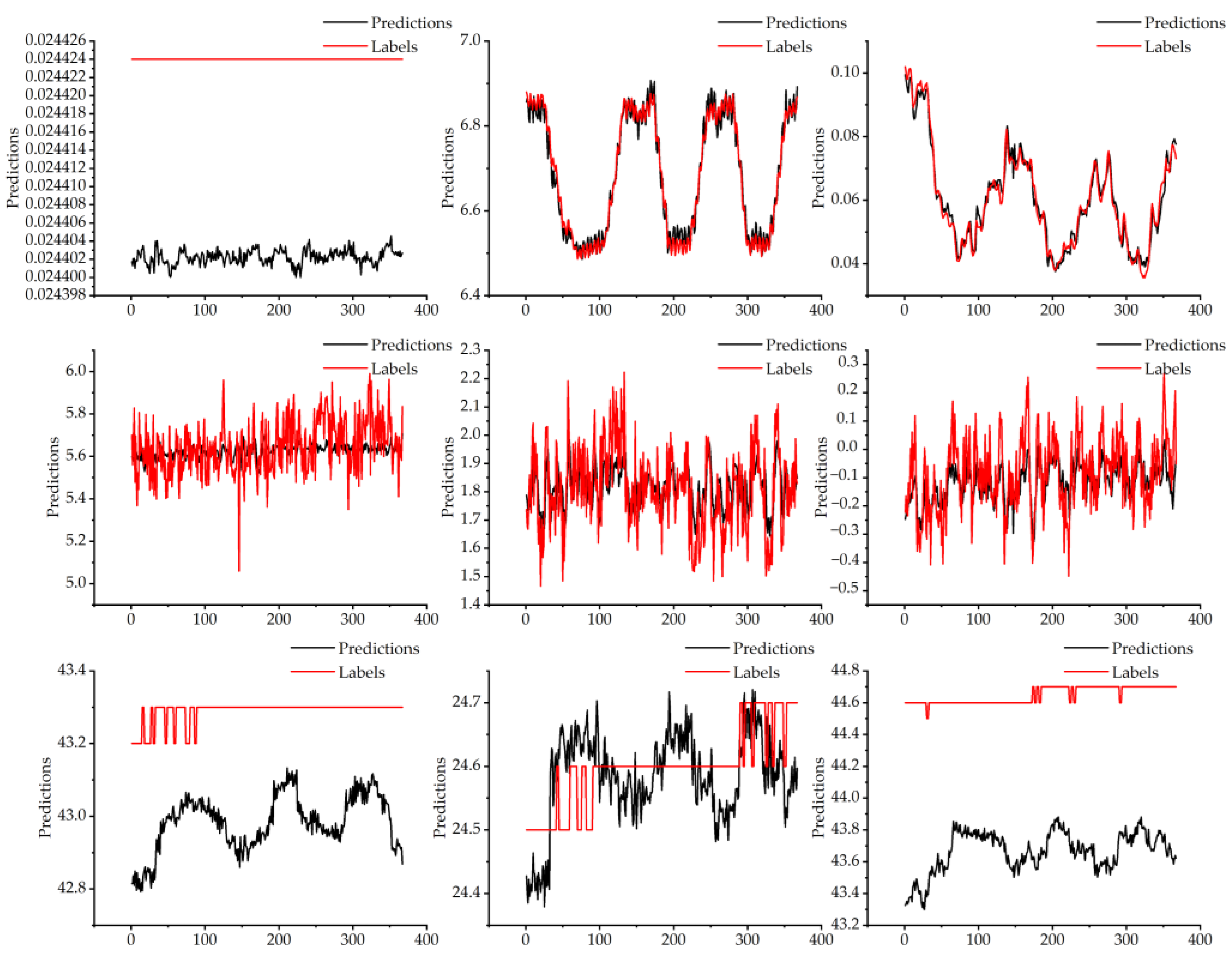
- The trained SE-ResNet-Transformer model is used to predict the CNC machine tool operating states. The actual and predicted CNC machine tool operating states are compared to evaluate the model.
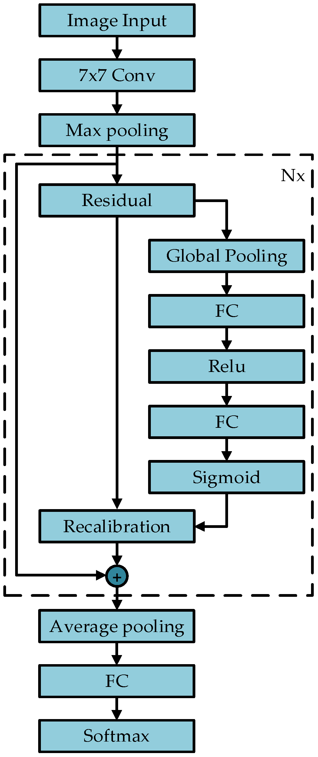
2.2. SE-ResNet
2.2.1. Squeeze-and-Excitation (SE)
2.2.2. ResNet
2.2.3. SE-ResNet
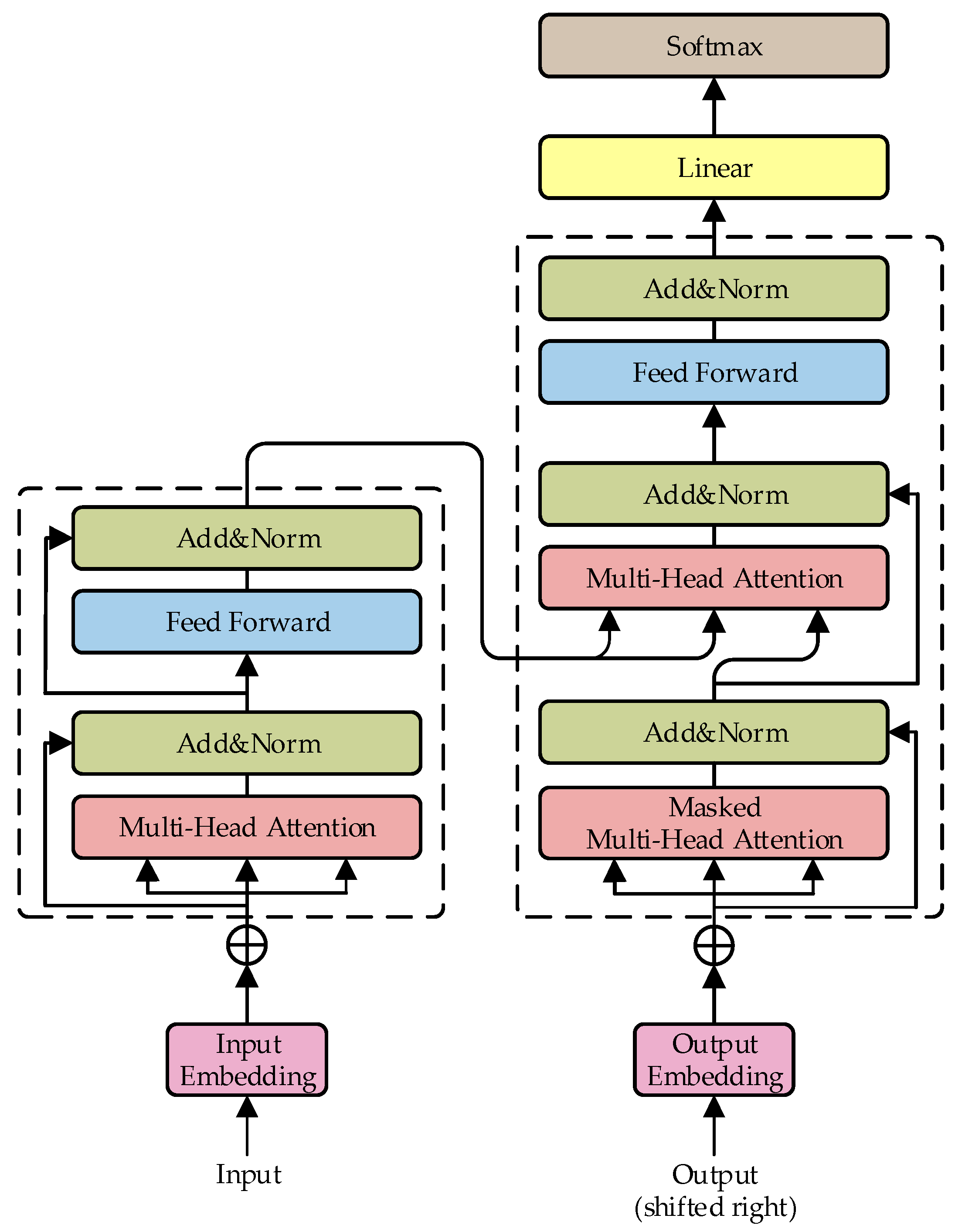
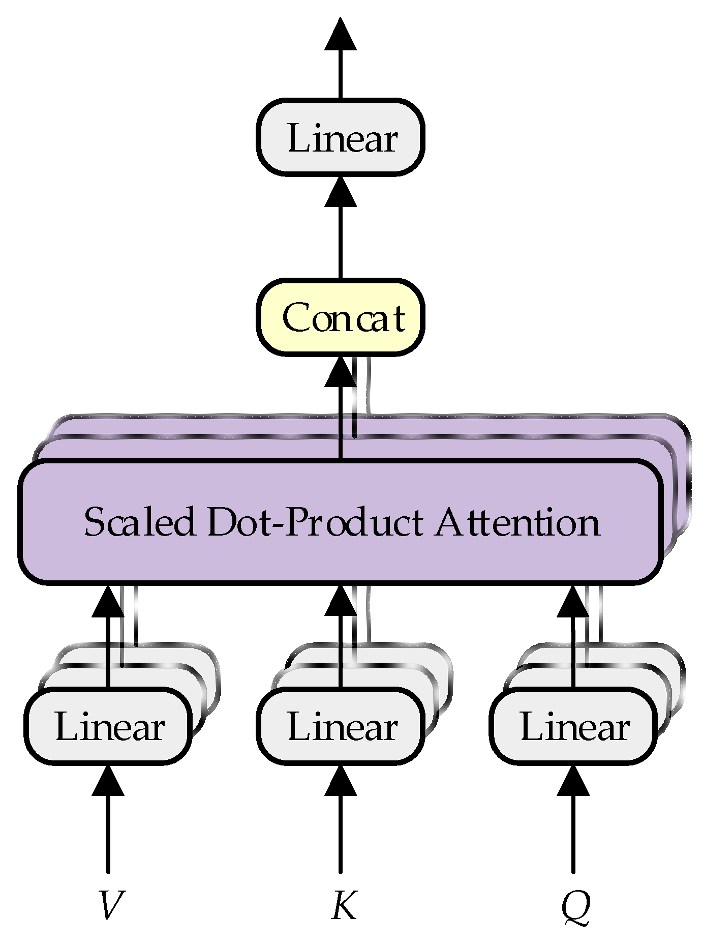
2.3. Transformer Model
2.4. Data Fusion
2.5. Workflow of SE-ResNet-Transformer Model
3. Experimental
3.1. Data Acquisition
3.2. Experimental
3.3. Experimental Results and Discussion
4. Conclusions
Author Contributions
Funding
Data Availability Statement
Conflicts of Interest
References
- Zhang, X.; Guo, Q.; Liu, S.; Cheng, C. Analysis and Prospect of Deep Learning Technology and Its Fault Diagnosis Application. J. Xi’an Jiaotong Univ. 2020, 12, 54. [Google Scholar]
- Chen, H.; Zhong, K.; Ran, G.; Cheng, C. Deep Learning-Based Machinery Fault Diagnostics. Machines 2022, 10, 690. [Google Scholar] [CrossRef]
- Zhu, J.; Liu, T. Bidirectional Current WP and CBAR Neural Network Model-Based Bearing Fault Diagnosis. IEEE Access 2023, 11, 143635. [Google Scholar] [CrossRef]
- Hao, F.; Wang, H.; Li, H. Fault diagnosis of rollingbearingbased on continuous hidden Markov model. Chin. J. Constr. Mach. 2019, 2, 17. [Google Scholar] [CrossRef]
- Ahmed, H.O.A.; Nandi, A.K. Convolutional-Transformer Model with Long-Range Temporal Dependencies for Bearing Fault Diagnosis Using Vibration Signals. Machines 2023, 11, 746. [Google Scholar] [CrossRef]
- Qian, L.; Pan, Q.; Lv, Y.; Zhao, X. Fault Detection of Bearing by Resnet Classifier with Model-Based Data Augmentation. Machines 2022, 10, 521. [Google Scholar] [CrossRef]
- Afridi, Y.S.; Hasan, L.; Ullah, R.; Ahmad, Z.; Kim, J.-M. LSTM-Based Condition Monitoring and Fault Prognostics of Rolling Element Bearings Using Raw Vibrational Data. Machines 2023, 11, 531. [Google Scholar] [CrossRef]
- Ströbel, R.; Probst, Y.; Deucker, S.; Fleischer, J. Time Series Prediction for Energy Consumption of Computer Numerical Control Axes Using Hybrid Machine Learning Models. Machines 2023, 11, 1015. [Google Scholar] [CrossRef]
- Moysidis, D.A.; Karatzinis, G.D.; Boutalis, Y.S.; Karnavas, Y.L. A Study of Noise Effect in Electrical Machines Bearing Fault Detection and Diagnosis Considering Different Representative Feature Models. Machines 2023, 11, 1029. [Google Scholar] [CrossRef]
- Deng, F.; Chen, Z.; Liu, Y.; Yang, S.; Hao, R.; Lyu, L. A Novel Combination Neural Network Based on ConvLSTM-Transformer for Bearing Remaining Useful Life Prediction. Machines 2022, 10, 1226. [Google Scholar] [CrossRef]
- Sun, S.; Peng, T.; Huang, H. Machinery Prognostics and High-Dimensional Data Feature Extraction Based on a Transformer Self-Attention Transfer Network. Sensors 2023, 23, 9190. [Google Scholar] [CrossRef] [PubMed]
- Rama, V.S.B.; Hur, S.-H.; Yang, Z. Short-Term Fault Prediction of Wind Turbines Based on Integrated RNN-LSTM. IEEE Access 2024, 12, 22465. [Google Scholar] [CrossRef]
- Chen, X.; Chen, W.; Dinavahi, V.L.; Liu, Y.; Feng, J. Short-Term Load Forecasting and Associated Weather Variables Prediction Using ResNet-LSTM Based Deep Learning. IEEE Access 2023, 11, 5393. [Google Scholar] [CrossRef]
- Wanke, Y.; Chunhui, Z.; Biao, H. MoniNet with Concurrent Analytics of Temporal and Spatial Information for Fault Detection in Industrial Processes. IEEE Trans. Cybern. 2022, 52, 8. [Google Scholar] [CrossRef] [PubMed]
- Wanke, Y.; Chunhui, Z. Broad Convolutional Neural Network Based Industrial Process Fault Diagnosis with Incremental Learning Capability. IEEE Trans. Ind. Electron. 2020, 6, 67. [Google Scholar] [CrossRef]
- Wanke, Y.; Chunhui, Z. Robust Monitoring and Fault Isolation of Nonlinear Industrial Processes Using Denoising Autoencoder and Elastic Net. IEEE Trans. Control Syst. Technol. 2022, 28, 3. [Google Scholar] [CrossRef]
- Wang, L.; Zhang, C.; Zhu, J.; Xu, F. Fault Diagnosis of Motor Vibration Signals by Fusion of Spatiotemporal Features. Machines 2022, 10, 246. [Google Scholar] [CrossRef]
- Yu, Z.; Zhang, L.; Kim, J. The Performance Analysis of PSO-ResNet for the Fault Diagnosis of Vibration Signals Based on the Pipeline Robot. Sensors 2023, 23, 4289. [Google Scholar] [CrossRef]
- Lu, Q.; Chen, S.; Yin, L.; Ding, L. Pearson-ShuffleDarkNet37-SE-Fully Connected-Net for Fault Classification of the Electric System of Electric Vehicles. Appl. Sci. 2023, 13, 13141. [Google Scholar] [CrossRef]
- Quan, S.; Sun, M.; Zeng, X.; Wang, X.; Zhu, Z. Time Series Classification Based on Multi-Dimensional Feature Fusion. IEEE Access 2023, 11, 11066. [Google Scholar] [CrossRef]
- Hongfeng, G.; Jie, M.; Zhonghang, Z.; Chaozhi, C. Bearing Fault Diagnosis Method Based on Attention Mechanism and Multi-Channel Feature Fusion. IEEE Access 2024, 12, 45011. [Google Scholar] [CrossRef]
- Fu, Y.; Chen, X.; Liu, Y.; Son, C.; Yang, Y. Gearbox Fault Diagnosis Based on Multi-Sensor and Multi-Channel Decision-Level Fusion Based on SDP. Appl. Sci. 2022, 12, 7535. [Google Scholar] [CrossRef]
- Liu, Y.; Xiang, H.; Jiang, Z.; Xiang, J. A Domain Adaption ResNet Model to Detect Faults in Roller Bearings Using Vibro-Acoustic Data. Sensors 2023, 23, 3068. [Google Scholar] [CrossRef]
- Zhu, J.; Zhao, Z.; Zheng, X.; An, Z.; Guo, Q.; Li, Z.; Sun, J.; Guo, Y. Time-Series Power Forecasting for Wind and Solar Energy Based on the SL-Transformer. Energies 2023, 16, 7610. [Google Scholar] [CrossRef]
- Chen, T.; Qin, H.; Li, X.; Wan, W.; Yan, W. A Non-Intrusive Load Monitoring Method Based on Feature Fusion and SE-ResNet. Electronics 2023, 12, 1909. [Google Scholar] [CrossRef]
- Shaheed, K.; Qureshi, I.; Abbas, F.; Jabbar, S.; Abbas, Q.; Ahmad, H.; Sajid, M.Z. EfficientRMT-Net—An Efficient ResNet-50 and Vision Transformers Approach for Classifying Potato Plant Leaf Diseases. Sensors 2023, 23, 9516. [Google Scholar] [CrossRef] [PubMed]
- Wang, N.; Zhao, X. Time Series Forecasting Based on Convolution Transformer. IEICE Trans. Inf. Syst. 2023, 5, 976. [Google Scholar] [CrossRef]
- Fei, M.; Zhijie, Y.; Jiangbo, W.; Qipeng, S.; Bo, B.; Qingyuan, G.; Kai, H. Short-term traffic flow velocity prediction method based on multi-channel fusion of meteorological and transportation data. J. Traffic Transp. Eng. 2024, 1, 17. Available online: http://kns.cnki.net/kcms/detail/61.1369.U.20240418.1116.002.html (accessed on 14 April 2024).
- Chungwen, M.; Jiangming, D.; Yuzheng, C.; Huaiyuan, L.; Zhicheng, S.; Jing, X. The relationships between cutting parameters, tool wear, cutting force and vibration. Adv. Mech. Eng. 2018, 10, 1. [Google Scholar] [CrossRef]
- Owais Qadri, M.; Namazi, H. Fractal-based analysis of the relation between tool wear and machine vibration in milling operation. Fractals 2022, 28, 6. [Google Scholar] [CrossRef]
- Fan, C.; Chen, H.; Kuo, T. Prediction of machining accuracy degradation of machine tools. Precis. Eng. 2012, 2, 288. [Google Scholar] [CrossRef]
- Li, C.; Song, Z.; Huang, X.; Zhao, H.; Jiang, X.; Mao, X. Analysis of Dynamic Characteristics for Machine Tools Based on Dynamic Stiffness Sensitivity. Processes 2021, 9, 2260. [Google Scholar] [CrossRef]
- Chen, C.; Qiu, A.; Chen, H.; Chen, Y.; Liu, X.; Li, D. Prediction of Pollutant Concentration Based on Spatial–Temporal Attention, ResNet and ConvLSTM. Sensors 2023, 23, 8863. [Google Scholar] [CrossRef] [PubMed]


| Layer Name | Output Size | 50-Layer |
|---|---|---|
| Conv1 | 112 112 | 7 7, 64, stride2 |
| Conv2_x | 56 56 | 3 3, max pool, stride2 |
| Conv3_x | 28 28 | |
| Conv4_x | 14 14 | |
| Conv5_x | 7 7 | |
| 1 1 | Average pool, 1000-d fc, softmax | |
| FLOPs | 3.8 109 | |
| CNC Machine Status | Spindle Speed (r/min) | Feed Rate (mm/r) | Depth of Cut (mm) |
|---|---|---|---|
| Normal state | 500 | 0.2 | 1 |
| Abnormal spindle speed | 200 | 0.2 | 1 |
| 1000 | 0.2 | 1 | |
| Abnormal depth of cut | 500 | 0.2 | 2 |
| Abnormal feed | 500 | 0.4 | 1 |
| Parameters | Value |
|---|---|
| Initial learning rate | 0.001 |
| Activation function | ReLU |
| Optimizer | Adam |
| Number of heads | 4 |
| Hidden size | 64 |
| Parameters of Machine Tools | R2 | MAE | RMSE | MAPE |
|---|---|---|---|---|
| Main motor current | 0.937 | 0.0184 | 0.023 | 0.027 |
| Cross-feed axis motor current | 0 | 6.05 × 10⁻⁵ | 6.74 × 10⁻⁵ | 0.0029 |
| Longitudinal feed axis motor current | 0.9709 | 0.0022 | 0.0026 | 0.0383 |
| Spindle vibration | 0.0421 | 0.0998 | 0.1247 | 0.176 |
| Cross-feed axis vibration | 0.2863 | 0.0976 | 0.1216 | 0.0543 |
| Longitudinal feed axis vibration | 0.3042 | 0.0874 | 0.1079 | 34.0182 |
| Main motor temperature | −97.4553 | 0.3047 | 0.3125 | 0.007 |
| Cross-feed axis temperature | 0.5784 | 0.063 | 0.0755 | 0.0025 |
| Longitudinal feed axis temperature | −366.764 | 0.9818 | 0.9891 | 0.0219 |
| Error Level | Cross-Feed Axis Motor Current | Main Motor Temperature | Cross-Feed Axis Temperature | Longitudinal Feed Axis Temperature |
|---|---|---|---|---|
| 0.00002 | 1.36% | - | - | - |
| 0.000021 | 50.40% | - | - | - |
| 0.000022 | 61.30% | - | - | - |
| 0.000023 | 94.84% | - | - | - |
| 0.000024 | 100% | - | 0 | - |
| 0.003 | - | - | 55.84% | - |
| 0.1 | - | 0 | 80.38% | - |
| 0.15 | - | 0.81% | 96.73% | - |
| 0.3 | - | 44.41% | 100% | - |
| 0.3047 | - | 69.75% | - | - |
| 0.4 | - | 94.27% | - | - |
| 0.5 | - | 99.72% | - | 0 |
| 1 | - | 100% | - | 54.22% |
| 1.1 | - | - | - | 83.10% |
| 1.2 | - | - | - | 95.36% |
| 1.3 | - | - | - | 99.72% |
| 1.4 | - | - | - | 100% |
| Method | SE-ResNet | ResNet50 | ResNet34 | GoogLeNet | AlexNet |
|---|---|---|---|---|---|
| Accuracy (%) | 98.56 | 97.89 | 92.21 | 92.45 | 93.41 |
Disclaimer/Publisher’s Note: The statements, opinions and data contained in all publications are solely those of the individual author(s) and contributor(s) and not of MDPI and/or the editor(s). MDPI and/or the editor(s) disclaim responsibility for any injury to people or property resulting from any ideas, methods, instructions or products referred to in the content. |
© 2024 by the authors. Licensee MDPI, Basel, Switzerland. This article is an open access article distributed under the terms and conditions of the Creative Commons Attribution (CC BY) license (https://creativecommons.org/licenses/by/4.0/).
Share and Cite
Wu, Z.; He, L.; Wang, W.; Ju, Y.; Guo, Q. A Fault Prediction Method for CNC Machine Tools Based on SE-ResNet-Transformer. Machines 2024, 12, 418. https://doi.org/10.3390/machines12060418
Wu Z, He L, Wang W, Ju Y, Guo Q. A Fault Prediction Method for CNC Machine Tools Based on SE-ResNet-Transformer. Machines. 2024; 12(6):418. https://doi.org/10.3390/machines12060418
Chicago/Turabian StyleWu, Zhidong, Liansheng He, Wei Wang, Yongzhi Ju, and Qiang Guo. 2024. "A Fault Prediction Method for CNC Machine Tools Based on SE-ResNet-Transformer" Machines 12, no. 6: 418. https://doi.org/10.3390/machines12060418
APA StyleWu, Z., He, L., Wang, W., Ju, Y., & Guo, Q. (2024). A Fault Prediction Method for CNC Machine Tools Based on SE-ResNet-Transformer. Machines, 12(6), 418. https://doi.org/10.3390/machines12060418