Abstract
Air conditioning contributes a high percentage of energy consumption over the world. The efficient prediction of energy consumption can help to reduce energy consumption. Traditionally, multidimensional air conditioning energy consumption data could only be processed sequentially for each dimension, thus resulting in inefficient feature extraction. Furthermore, due to reasons such as implicit correlations between hyperparameters, automatic hyperparameter optimization (HPO) approaches can not be easily achieved. In this paper, we propose an auto-optimization parallel energy consumption prediction approach based on reinforcement learning. It can parallel process multidimensional time series data and achieve the automatic optimization of model hyperparameters, thus yielding an accurate prediction of air conditioning energy consumption. Extensive experiments on real air conditioning datasets from five factories have demonstrated that the proposed approach outperforms existing prediction solutions, with an increase in average accuracy by 11.48% and an average performance improvement of 32.48%.
1. Introduction
In recent years, with the rapid development of the global economy, building energy consumption has shown a steady increase, where air conditioning contributes around 50–60% []. Therefore, predicting the energy consumption of building air conditioning systems is crucial for reducing the total amount of energy consumption. Traditional energy consumption prediction (ECP) methods including autoregression(AR) [], structural time series models []—which usually need strong domain expertise to build appropriate models—or require extensive crossvalidation computations over a large set of parameters [].
Some deep learning-based ECP methods are capable of learning complex data representations and learning function forms in a data-driven manner [], thereby reducing the need for manual feature engineering and model design. Bai et al. [] proposed using Temporal Convolutional Networks (TCNs) for sequence modeling to enhance the learning ability for time series data. However, with the scale and dimensionality of the collected air conditioning energy consumption datasets increasing, these existing ECP methods usually have low efficiency [] when they sequentially extract features from time series data when training prediction models.
Additionally, deep learning-based ECP methods also contain many hyperparameters that need to be dynamically optimized, which requires a decent amount of time. Traditional manual tuning or grid search methods are often inefficient and time-consuming []. Evolution strategies, Bayesian optimization, Hyperband, and reinforcement learning [] may be a good help for such problem. However, the existing hyperparameter optimization methods face limitations in capturing implicit correlations among multiple hyperparameters [].
To address the above challenges, we propose a reinforcement learning based auto-optimized parallel prediction (RL-AOPP) approach for air conditioning energy consumption, which can extract data features in parallel during the prediction process and achieve the automatic optimization of model hyperparameters. In RL-AOPP, a prediction model based on a multidimensional temporal convolutional network (MTCN) is employed to extract the features of multidimensional data in parallel, thus preserving their temporal relationships. Another model of RL-AOPP is a deep reinforcement learning-based HPO model, which can progressively optimize decision-making strategies through interaction with the environment in the complex hyperparameter search space of the prediction model, thus achieving an efficient and accurate HPO process.
The contributions of this paper are as follows:
- We propose an innovative reinforcement learning based auto-optimized parallel prediction approach for air conditioning energy consumption.
- We design a multidimensional causal expansion convolutional network with enhanced activation function, thus achieving efficient extract timing characteristics in large scale air conditioning datasets.
- An HPO model is designed based on an improved actor network and a differential value sample pool construction module, which can improve the convergence speed of the model.
- We evaluate our approach using real datasets from five air conditioning factories, and the results indicate that the proposed approach outperforms existing prediction methods in terms of accuracy and performance.
2. Related Work
In this section, we will introduce prior research on time series data prediction and hyperparameter optimization.
2.1. Time Series Data Prediction
Time series data exhibit characteristics such as periodicity, trend, and irregularity along the temporal dimension []. Chaerun et al. [] compared the effectiveness of machine learning and deep learning in ECP. Lyu et al. [] proposed a multistep prediction method based on Long Short-Term Memory (LSTM), which successfully captured the periodicity and temporal patterns. Ewees et al. [] employed a Heap-Based Optimizer (HBO) to train a LSTM network and further enhanced the predictive capability of the original LSTM model. Abbasimehr et al. [] introduced a hybrid model that combines LSTM networks with multihead attention mechanisms, thus facilitating the precise prediction of intricate nonlinear time series data.
To further enhance the learning capability for time series data, Bai et al. [] proposed the utilization of TCN for series modeling. Experimental results indicated that TCN outperformed typical recurrent networks such as LSTM and exhibited longer effective memory. Bian et al. [] introduced the TCN-BP model, which can extract the latent relationship between time series data and non-time series data. Limouni et al. [] introduced a hybrid model LSTM-TCN, thus achieving more accurate power prediction. Huang et al. [] devised a convolutional differential network based on temporal subsequence, which enhances the predictive capability of TCN. Liu et al. [] introduced a short-term load prediction approach grounded in TCN and dense convolutional networks.
These existing approaches can only sequentially extract feature information when facing multidimensional temporal data, thus leading to low training efficiency.
2.2. Hyperparameter Optimization
Well-performing hyperparameter configurations [] are necessary for efficient prediction. Bayesian optimization serves as an approximate method and finds extensive application in HPO. Snoek et al. [] applied Bayesian optimization to the process of hyperparameter tuning, thus enhancing the performance of CNN in classification tasks. Feurer et al. [] introduced a hyperparameter-free ensemble model based on Bayesian optimization, which reduces optimization time.
Due to latent mapping relationships between hyperparameters and models, the above methods perform poorly in finding the optimal configuration of hyperparameters. Therefore, some researchers consider abstracting the HPO process into a Markov decision process [] to introduce reinforcement learning. For instance, Jomaa [] proposed a reinforcement learning approach to sequentially optimize hyperparameters, thus eliminating the need for heuristic acquisition functions. Liu [] proposed a reinforcement learning optimization method for efficient hyperparameter tuning, which reduces the search space and improves efficiency.
However, the long sequence dependency of time series prediction makes the return signal of reinforcement learning sparse and delayed, which makes it difficult to learn optimal hyperparameters [] for time series prediction scenarios.
3. Design of the Reinforcement Learning-Based Auto-Optimized Parallel Prediction Approach
In this section, we first introduce the overall architecture of the RL-AOPP. Then, we separately introduce the prediction model, the hyperparameter optimization model, and the detailed workflows of RL-AOPP.
3.1. Architecture
Time series data differ from other types of data, as they exhibit characteristics such as periodicity, trend, and irregularity in the temporal dimension. Currently, mainstream time series prediction methods still face challenges when dealing with complex time series data, especially air conditioning energy consumption. On the one hand, the dataset collected by sensors has a complex structure and spans a large time dimension, which leads to the feature information among multiple variables becoming blurred or even disappearing during model training. On the other hand, the original network structure of temporal convolutional networks cannot simultaneously handle multidimensional data inputs and struggles to fully extract the latent information among multivariate time series, thus resulting in the poor predictive ability of the algorithm. Therefore, we propose a time series prediction model called MTCN, which addresses the challenges in handling multidimensional data and relieves the phenomenon of disappearing correlations among multiple variables.
However, several layers in the MTCN structure may lead to performance issues such as vanishing or exploding gradients during model training. To address this, we propose an activation function called Parameter Softplus (PSoftplus), which not only effectively mitigates the aforementioned problems but also improves model performance.
Furthermore, the time series prediction methods involve many hyperparameters. Due to the unclear mapping relationships between hyperparameters and models, it is necessary to continuously adjust hyperparameters based on the accuracy of the model. This process consumes a lot of time and computational resources. Therefore, an HPO model called Differential Sampling and Long Short-Term Memory-Based Deep Reinforcement Learning (DSLD) has been designed, which has been integrated with the MTCN model to achieve HPO during the model prediction process.
The architecture of RL-AOPP is shown in Figure 1, which mainly includes a prediction model MTCN and a hyperparameter optimization model DSLD. The two models are integrated by using hyperparameter combinations and accuracy values as the signal quantities for communication.

Figure 1.
The Architecture of RL-AOPP Framework.
The MTCN consists of the residual blocks and a fully connected layer. The residual blocks in the MTCN are designed to enable the working of time series data prediction. The fully connected layer is responsible for implementing conversion from the input dimension to the output dimension. The main components of the residual blocks include multidimensional causal dilation convolution, a PSoftplus activation function, and a residual connection. To achieve parallel feature extraction, we use multiple multidimensional causal dilation convolutions, which bring many layers in the MTCN. Philipp et al. [] proved that excessive layers can lead to gradient explosion or the vanishing phenomenon. Psoftplus can standardize the output means to around zero, thereby alleviating the above problem. The introduction of the residual connection allows the network to pass information across layers, thus making the training of deep networks more effective.
The DSLD mainly includes two parts. The first part consists of a differential value experience sample pool (DS-POOL), which can reduce the correlation among the input samples. The remaining part contains four modules: the actor network, the critic network, and two target networks that are created on the policy network and value network, respectively. The model update process primarily involves updating the parameter values of the above four modules. The policy network is updated by maximizing the cumulative expected reward value—the maximum return—while the value network is updated by minimizing the error between the output value and the target value as much as possible. The parameter update of the target network adopts a soft update method and introduces a soft interval update coefficient. The update is carried out by weighting the original target network parameters and the new corresponding network parameters.
The overall workflow of the RL-AOPP framework is shown in Figure 1:
- The DLSD completes the initialization of hyperparameters and prepares the multidimensional energy consumption data (1.1).
- The data are fed into the causal dilated convolutional network for feature extraction and processed nonlinearly by the PSoftplus activation function (1.2).
- The results are passed to the next layer of the network through the residual structure (1.3).
- After updates through multiple residual blocks, the output is generated by the fully convolutional network (1.4).
- After each iteration of the model training, the final accuracy value is passed to the DSLD model as a reference for the next iteration (1.5–1.6).
- The DSLD model sorts the interacted samples according to their value and stores them in the DS-POOL (2.1).
- When the number of samples in the buffer pool reaches the maximum limit, the DSLD model will perform one round of internal parameter updates of the network structure (2.2–2.5).
- After the action decision network makes a decision, the hyperparameter configuration in the decision content is passed to the MTCN model (1.1).
In the subsequent iterations, the MTCN model will use this hyperparameter configuration to train.
3.2. Design of the Parallel Prediction Model
To improve the performance of data feature extraction, we propose multidimensional causal dilated convolution (MCDC), which consists of multidimensional convolution kernels (MCKs). Because the MCKs can retain the temporal characteristics of one-dimensional data, we can consider it as composed of multiple one-dimensional convolution kernels, with the number of these kernels determined by the number of features in the data sample. During the sliding process of the multidimensional convolution window, the convolution process of the kernel that corresponds to each dimension is independent. Consequently, the MCKs can receive data from all dimensions in parallel, thus achieving full coverage of the data features.
To explain the structure of the MCKs, suppose that the energy consumption dataset has m-dimensional features and a sample length of n, i.e., . The dimension of the convolutional kernel is m, and the length is k. In addition, the weight of the convolutional kernel is set to , where . In each single layer, after the data pass through the convolution operation of the current window of the MCK, a feature matrix with a corresponding dimension of can be output, i.e., . By traversing the feature matrix, we calculate the convolution result at each position, which is given by the Equation (1). The final output is the feature matrix O after the convolution operation.
The MCKs can not only extract temporal information but also ensure that the correlations between multivariables will not become blurred or even disappear due to multiple convolution operations while extracting multivariable feature information. This is because, during the actual training process, the input data undergo multiple convolution operations through multidimensional dilated causal convolution, which means that the information received by higher-level computing units contains the information extracted from the initial input. In other words, all the inputs have already undergone convolution operations from the beginning, thus highlighting the main features. Then, the higher-level network eventually extracts the temporal information and multidimensional feature information of the data samples.
In the scenario where MCDC is not applied, the data need to be entered sequentially. As shown in Figure 2a, each computing unit will only calculate the input content at the current moment and receive the next input in sequence. For multidimensional data such as air conditioning energy consumption time series datasets, traditional computational processing is very time-consuming. To address the above problem, we proposed the MCK, which follows the parallel method in Figure 2b. Each dimension of data is no longer input separately, which can achieve parallel processing of multidimensional time series data.

Figure 2.
The processing flow of the calculation unit in MTCN: (a) The convolutional kernel first extracts features from the red region, and only in subsequent iterations does it sequentially extract features from the blue and purple regions. (b) Within a single iteration, the kernel can extract features in parallel from red, blue, and purple regions while preserving the original temporal characteristics of the data.
To solve the problem of gradient explosion or vanishing caused by too many layers in the network, we propose PSoftplus as the activation function. Firstly, we shift the Softplus downward to achieve negative output values for some input data, thus lowering the overall mean. Then, we set the coefficient to alleviate the problem of gradient vanishing []. When the input , adjusts the curve slope of the function image. When , it affects the saturation position of the function. The formula for the PSoftplus activation function is shown in Equation (2).
Among them, if > 0, can adjust the slope of the function graph curve for positive values, and for negative values, it can affect the saturation position of the function. The larger the value of , the more the function is greater than zero, which will to some extent alleviate the problem of gradient disappearance. To ensure that the improved activation function can cross zero, is set to 0, as shown in Equation (3). By solving Equation (3), it shows that .
The equation for the PSoftplus is shown in Equation (4), and the function figure is shown in Figure 3.

Figure 3.
PSoftplus activation function.
In the backpropagation process of the MTCN convolutional neural network, the actual gradient values reaching the bottom layer after layer-by-layer computation will become smaller or larger. The rate of this change is determined by the derivative of the activation function, which is calculated based on the number of computations. Assuming the number of computations during the training process is n, the formula for calculating the rate of change of the network gradient is shown in Equation (5).
Equation (5) proves that the parameter determines the gradient propagation speed and affects the network training performance.
To explain why the improved activation function alleviates the mean shift problem, we assume that the actual input values set of the activation function is x, and we use the set to represent the probability of the corresponding input value. In addition, the input values contain positive and negative values, which we represent as and , respectively. The PSoftplus activation function is shown in Equation (6). Compared to the Softplus function, the parameters and are always greater than zero, and , which makes the mean output of the PSoftplus function closer to zero.
3.3. Design of the Reinforcement Learning-Based Hyperparameter Optimization Model
In this section, we first provide a detailed introduction to the DSLD hyperparameter optimization model, including the design of the actor network and the DS-POOL. Then, we introduce the implementation details of the RL-AOPP framework.
3.3.1. Markov Decision Process and Construction of Actor Network
The hyperparameter optimization problem refers to selecting a specific value for each hyperparameter of the model to be optimized within its search space, thus combining them into a set of hyperparameter combinations and applying them to model training. For the ECP problem to be solved in this paper, the goal of hyperparameter optimization is to find a set of hyperparameter settings in the hyperparameter search space that minimizes the error and maximizes the accuracy of the final trained prediction model. The objective function can be expressed as Equation (7).
In this equation, is the training set, is the validation set, is the model obtained by training on the training set with hyperparameter configuration , and L is the loss function of M in this task.
We can formulate the hyperparameter optimization problem in ECP as a Markov decision process (MDP). In this process, an optimal value needs to be determined for each hyperparameter of the model, thus ultimately obtaining an optimal hyperparameter vector. Suppose the model M to be optimized has N hyperparameters to be selected. If we consider the hyperparameter selection problem as a multiarmed bandit problem, and the search space for the ith hyperparameter is , then the entire search space is . This search space is high-dimensional and complex, and it tends to grow exponentially with the increase in the number of hyperparameters.
To solve the problem of an overly large problem space, the idea of divide and conquer is adopted to optimize the N hyperparameters separately. In reinforcement learning, we can choose different hyperparameters at different time steps, for example, selecting the t-th hyperparameter at time step t. However, separate decision making may lead to the neglect of the correlations between the hyperparameters. Therefore, this paper proposes to use the LSTM, which has the characteristic of analyzing the intrinsic connections in time series data as the core structure of the actor network. This allows each hyperparameter selection to be based on the decision of the previous hyperparameter selection, thus converting the hyperparameter selection process into a sequential decision-making process. The entire search space becomes , and the simplified search space only increases linearly with the increase in hyperparameters, thus greatly reducing the search space and improving the search rate.
If the model can predict the trend of the next hyperparameter selection direction, it can avoid some values that will not be selected in the future. Consequently, we redesign the structure of the actor network, which is shown in Figure 1-Actor. The Actor consists of two layers of LSTM and two layers of fully connected layers (FCLs). The fully connected layers are used to adjust the dimensions of the input and output, while the LSTM layers are used to learn the latent information present in the input data and to preserve its variation trend in the time dimension. For an optimization problem containing N hyperparameters, at a certain moment t, the actor network selects the hyperparameter based on the input current state . After N time steps, the network obtains a set of hyperparameter configurations . Consequently, a complete epoch at the current moment includes N time steps. Then, the action sequence interacts with the environment. The model to be optimized uses the hyperparameter combination selected at the current moment to train the model, and the accuracy of the model on the validation dataset is used as the reward value at the current moment.
Therefore, the Markov decision process for the hyperparameter optimization problem will be redefined, and the target object is a model containing N hyperparameters to be optimized:
Action space: The actor network will use N time steps, thus selecting the value of the ith hyperparameter at the ith time step, , until the end of the Nth time step to obtain a set of hyperparameter combinations. For each hyperparameter i within the N time steps, its search space is . The overall search space is .
State space: The environment includes the model to be optimized, the dataset, and the hyperparameter combination. During the execution of the optimization task, only the hyperparameter combination to be optimized is dynamically adjusted. Therefore, the hyperparameter setting of the algorithm at the previous moment is chosen to be marked as the state at the current moment.
Reward value: The accuracy of the trained model on the validation dataset using a set of actions A is used as the reward value. , where the value of is the accuracy of the MTCN model.
State transition probability: The transition probability of the environment state is not observable. Therefore, this research method adopts a model-free deterministic policy gradient approach for learning.
Discount factor: This value will be reflected in the calculation of the cumulative return value. The closer it is to 1, the longer the current network considers future benefits.
3.3.2. Construction of Differential Value Experience Sample Pool
To reduce the correlation problem among samples in the experience sample pool, we propose a method for constructing a differential value experience sample pool with a high-value priority sampling experience replay mechanism. The experience samples are stored in the experience pool according to their learning value.
During the training process of the DSLD model, the actor network selects the hyperparameter actions, and the critic network gives the value that the selected actions may produce. After the actor network selects actions and interacts with the environment, the obtained samples are first used to calculate the temporal difference error (TDError) of the action value function before being put into the sample pool. Then, the experience samples are stored in the experience pool in order of this value. The value calculation formula is shown in Equation (8).
In the equation, represents instant reward and represents the action of the target policy in state . Our goal is to make as small as possible, which represents the difference between the current Q value and the target Q value of the next step. When is relatively large, it indicates that the sample has a significant influence on the value network, and it can be understood that this sample has a higher value. The probability of each experience sample being sampled depends on its value. The sampling probability of the jth sample is defined as , as shown in Equation (9).
In , is the rank of sample j in the replay experience pool according to the j value. The parameter is used to control the degree of priority usage, and and indicate fully greedy sampling based on priority. During the learning process, high-value samples have a positive impact on the network, but low-value samples cannot be ignored either. The definition of sampling probability can be seen as a method of introducing random factors when selecting experiences, because even low-value experiences may be replayed, thus ensuring the diversity of sampled experiences. This diversity helps prevent overfitting of the neural network. To correct the estimation bias caused by priority sampling, the loss function Loss of the estimation network is multiplied by the importance sampling weight , as shown in Equation (10).
In the equation, N represents the size of the differential value sample pool, and is used to adjust the distribution of weights. The higher the value of the sample, the higher its priority, and the smaller the importance sampling weight value, which smoothes the optimization surface by correcting the loss. Therefore, the differential value experience sample pool allows the algorithm to focus more on high-value samples and accelerate the convergence of the algorithm.
At this point, the DSLD optimization model can search for the optimal hyperparameter configuration of the MTCN prediction model. For a given air conditioning ECP model, all internal parameters of the networks are initialized. The DSLD policy network selects appropriate actions (hyperparameter combinations) and sets them as the hyperparameter values of the MTCN model. The MTCN is trained on the data sample set, and then the model is validated on the validation data samples to obtain accuracy. The action and reward are combined as an experience sample for the DSLD model and stored in the sample pool according to the rules based on the differential value. When the sample pool reaches a certain condition, data samples are sampled to update the internal parameters of the value network and policy network. After multiple iterations, the RL-AOPP framework can select a better hyperparameter configuration to achieve the highest prediction accuracy under the current task and output the prediction model under this configuration.
Algorithm 1 presents the complete training process of the RL-AOPP framework.
| Algorithm 1 RL-AOPP process |
|
4. Evaluation
Firstly, we verify the effect of RL-AOPP and find the optimal hyperparameter configuration. Secondly, we verify the advantages of the prediction model MTCN compared to other traditional prediction models. Thirdly, we validate the effectiveness of the optimization model DSLD.
4.1. Experiments Setup
Dataset: Our proposed method has been applied to all 596 magnetic levitation water machine air conditioning production factories across the country, and the data were managed using the E-plus data management platform. We selected six representative air conditioning datasets from the platform with a time interval of December 2020 to December 2023 for experimentation. The details of the experimental datasets are shown in Table 1.

Table 1.
Introduction to experimental datasets.
The air conditioning operation data have 12-dimensional sensor parameters, which have a strong correlation with the energy consumption of the air conditioning and are screened out from the multidimensional operation sensor parameters as the features of the experimental data samples. To meet the real-time monitoring of air conditioning energy consumption, this paper used the operation data of air conditioning within twenty minutes to predict the energy consumption situation for one hour.
Baseline: In the HPO experiment of the RL-AOPP framework, we selected CNN, RNN, LSTM, TCN, and MTCN as comparative models, and the hyperparameter search space for each model is shown in Table 2. We chose common hyperparameter optimization methods, including Bayesian-based optimization, using the Tree-Structured Parzen Estimator (TPE), grid search, and random search optimization for comparative experiments.
Table 2.
Hyperparameter search space of models.
Model: In the MTCN prediction experiment, the models were built by Keras. The CNN model has a convolutional kernel size of 4, a learning rate of 0.01, a batch size of 200, a dropout of 0.3, and an epoch of 50. The LSTM model has 50 neurons per layer, a dropout of 0.2, a learning rate of 0.001, a batch size of 70, and an epoch of 50. The RNN model has a learning rate of 0.001, a dropout of 0.3, a batch size of 70, and an epoch of 50. Both the TCN and the MTCN models have a learning rate of 0.05, an epoch of 50, a dilation rate of 2, a convolutional kernel size of 3, and the number of residual blocks is 4. At the same time, the MTCN model with ReLU was used as a comparison.
Other: The experiment adopted ten-fold crossvalidation and recorded the average value of the validation results. We used the early stopping method to prevent overfitting, thus continuously monitoring the accuracy in each iteration. When there was no significant improvement in performance or when it began to decline for three iterations, we stopped training and saved the model parameters.
Configuration: The server used in the experiments is a typical PC equipped with an Intel Core i9-9900k processor, an NVIDIA GeForce RTX 3090 graphics card, and 16 GB RAM. The Python version used in the experiments is 3.8.10, and the TensorFlow version is 2.12.0. The detailed software and hardware conditions are shown in Table 3.
Table 3.
Experiment environment.
4.2. Experiments on RL-AOPP Framework
To demonstrate the advantages of the DSLD compared to other traditional HPO methods, the experimental results of using different method combinations for hyperparameter optimization and predictive model training are shown in Table 4.
Table 4.
Prediction performance of MTCN on different datasets.
Comparing the results of RMSE, all optimization methods found hyperparameter configurations that performed better than the default parameter settings. The DSLD achieved a higher degree of model hyperparameter optimization compared to the other optimization methods in most tasks. From the time perspective, the grid search was computationally intensive. Random search had a low probability of finding the best configuration based on random sampling, thus resulting in a longer training time. The TPE combined with prior parameter information for updating, thus requiring fewer iterations and less training time. The internal structure of the DSLD reduced the search space, thus resulting in a faster average speed compared to the other aforementioned models. The experimental results demonstrate that this method can find the best hyperparameter configuration with low prediction error while reducing the search time and action space.
Furthermore, we applied the RL-AOPP algorithm to the Hong Kong dataset and conducted automatic hyperparameter optimization in the hyperparameter search space, as shown in Table 2, thus obtaining the best hyperparameter configuration for various models during the training process, as shown in Table 5.
Table 5.
The best hyperparameters for each model.
Based on the experimental results, we set the value of PSoftplus- at 1.5, thus indicating the most suitable activation function for this experiment, as shown in Equation (11).
4.3. Experiments on MTCN Model
4.3.1. Prediction Effectiveness of MTCN
To compare the prediction performance of the MTCN with other traditional prediction methods on the air conditioning energy consumption dataset, we conducted a comparative experiment on the prediction effects of multiple models, thus using the MAE and RMSE as evaluation metrics. The experimental results are shown in Table 6.
Table 6.
Prediction performance of RL-AOPP on different datasets.
The MTCN-PSoftplus in the table refers to the model we proposed, which is represented by MTCN in the following text. Overall, the MTCN prediction indicators were better than other models on all datasets. Comparing MTCN with TCN, the MAE values of MTCN in the five tasks were all smaller than the MAE values of TCN, with an average improvement of 6.7% in prediction accuracy. This result indicates that the causal convolution and dilated convolution structures of the MTCN model fully capture the temporal features in the dataset. Since the improved PSoftplus activation function alleviates the mean shift phenomenon, the MAE of MTCN was improved compared to MTCN-ReLU.
To more clearly illustrate the effectiveness of the MTCN model in ECP, the partial sample prediction results of the traditional CNN, RNN, LSTM models, and the MTCN model on the Hong Kong dataset are visualized as shown in Figure 4.

Figure 4.
Visualization of prediction results for different models.
From the comparison of the results, we can see that the CNN model could learn the features of data samples, but it was not sensitive to time series data, thus resulting in large fluctuations in the prediction results. After introducing the memory function, the prediction effect of the RNN model was better than the CNN model. However, due to the gradient vanishing problem during error backpropagation, the RNN could not effectively learn the features of early data, and some samples had large errors. The addition of the gate structure in LSTM enabled it to perform better than RNN in longer sequences, but based on the fitting curve, there were still many samples that deviated from the true values. Under this data distribution, the overall predicted values of the MTCN model are highly consistent with the true values, and there are no significant range error situations.
4.3.2. Validating PSoftplus Activation Function
To further verify the impact of the improved activation function PSoftplus on the MTCN prediction model, under the same experimental environment such as network structure, experimental dataset, and network parameter configuration, a comparative experiment of MTCN-ReLU, MTCN-Softplus, and MTCN-PSoftplus was conducted. This experiment selected part of the data samples from the Hong Kong dataset as the experimental dataset. The model training process is shown in Figure 5.
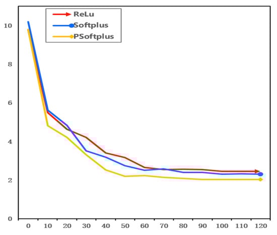
Figure 5.
Model convergence graph under different activation functions.
For this particular dataset, the training process illustrated demonstrates that the PSoftplus function converged faster than the Softplus function. The loss value of PSoftplus was smaller compared to both ReLU and Softplus. The ReLU activation function exhibited a zero gradient when the input was negative, thus potentially causing certain neurons to cease updating. Conversely, the Softplus activation function circumvented this issue by yielding nonzero outputs. However, this characteristic may lead to the activation values of subsequent layers diverging from zero, thereby also potentially impeding the convergence rate. The PSoftplus had an output mean close to zero and effectively utilized the output information, thus enhancing the convergence speed of the network while reducing network error.
4.4. Experiments on DSLD Model
To validate the advantages and effectiveness of the action decision network and the differentiable value sampling pool structure employed by the DSLD model in the domain of HPO, the DSLD, LDDPG, DSDDPG, and DDPG models were applied to the MTCN model for prediction, respectively. The experimental results are shown in Table 7.
Table 7.
The DSLD ablation experimental results on different datasets.
Compared to the DDPG, the DSLD achieved an average reduction of 2.06 in the RMSE and an average decrease of 1.61 in training time. This validates the superiority and effectiveness of the improved actor network and the differentiable value sampling pool structure in the field of HPO.
To further illustrate the advantages of the differentiable value sampling pool, the training processes of the two frameworks on Hong Kong and Shenzhen datasets are shown in Figure 6 and Figure 7, respectively.

Figure 6.
Training comparison graph of two frameworks in Hong Kong dataset.

Figure 7.
Training comparison graph of two frameworks in Shenzhen dataset.
In the Hong Kong dataset, although the LDDPG model also achieved high reward values, its training process was oscillatory. The model converged around the 350th epoch, with a slow convergence speed. In the Shenzhen dataset, while the LDDPG model found good reward values in the early stage, the model experienced significant oscillations in the subsequent experimental process and converged around the 240th epoch. The DSLD model converged around the 200th epoch, thus achieving rapid convergence during training, and had a stable training process.
To verify the impact of the control parameter on the convergence speed, we conducted comparative experiments by setting the control parameter to 0.3, 0.5, and 0.6, respectively. We show the training process of the MTCN model optimized by the DSLD model with different control parameters on the Hong Kong and Shenzhen datasets in Figure 8.

Figure 8.
Different control parameters comparison of DSLD model.
It can be observed that there is a strong correlation between the control parameter and model performance. The overall performance of the DSLD model with different control parameters was better than the original network, and the best control parameter setting is = 0.5. Analyzing the training process on the Shenzhen dataset, when = 0.3, the model obtained good rewards around the 210th epoch. When = 0.5, it converged around the 200th epoch, which was much faster than when = 0.3. However, the size of was not entirely positively correlated with model performance. For instance, when = 0.6, although the model obtained high rewards around the 180th epoch, it exhibited oscillations during the optimization process. Moreover, even after convergence around the 201st epoch, the model still experienced slight oscillations. The same phenomenon can be observed in the Hong Kong dataset. The reason is that this value was used to control the degree of priority sampling usage. The higher the value is set, the more valuable the high-value sample data are. However, frequent sampling leads to imbalanced data types during the training process, thus ultimately affecting algorithm performance.
5. Conclusions
In this paper, we proposed a reinforcement learning-based auto-optimization parallel energy consumption prediction approach called RL-AOPP. It can address the challenges brought by multidimensional time series data and hyperparameter optimization in the scenario of air conditioning energy consumption prediction, improve the performance of the training process, and efficiently find optimal hyperparameter configurations. Through extensive experiments, we evaluated the effectiveness of this approach.
However, the parallel processing mechanism of MTCN cannot solve the problems of high noise, excessive abnormal data, and data loss in the original air conditioning data, and it still requires complex data cleaning work. Furthermore, although we have optimized the performance of deep reinforcement learning, when there are too many hyperparameters in the algorithm, an amount of training time and computational resources are still required.
In the future, we are planning to use the large language model (LLM) integrated with our approach to provide comprehensive solutions for air conditioning ECP.
Author Contributions
Conceptualization, C.G., Y.M. and T.W.; Data curation, S.Y.; Formal analysis, C.G. and Y.M.; Funding acquisition, Y.T. and W.Z.; Investigation, Y.T.; Methodology, C.G., S.Y. and T.W.; Project administration, Y.M., Y.T., Y.L. and W.Z.; Resources, Y.T.; Supervision, Y.L., Z.B., B.Z., T.C. and W.Z.; Validation, C.G. and S.Y.; Visualization, C.G., S.Y. and T.W.; Writing—original draft, C.G., S.Y. and Y.M.; Writing—review and editing, Y.M., Y.L., Z.B., B.Z. and W.Z. All authors have read and agreed to the published version of the manuscript.
Funding
This research was funded by the National Natural Science Foundation of China under number 62072469.
Data Availability Statement
The data are contained within the article.
Conflicts of Interest
The author Chao Gu was employed by Qingdao Haier Air Conditioner ELEC, Co., Ltd. The remaining authors declare that the research was conducted in the absence of any commercial or financial relationships that could be construed as potential conflicts of interest.
References
- Zhao, T.; Qu, Z.; Liu, C.; Li, K. BIM-based analysis of energy efficiency design of building thermal system and HVAC system based on GB50189-2015 in China. Int. J. -Low-Carbon Technol. 2021, 16, 1277–1289. [Google Scholar] [CrossRef]
- Box, G.E.; Jenkins, G.M.; Reinsel, G.C.; Ljung, G.M. Time Series Analysis: Forecasting and Control; John Wiley & Sons: Hoboken, NJ, USA, 2015. [Google Scholar]
- Harvey, A.C. Forecasting, Structural Time Series Models and the Kalman Filter; Cambridge University Press: Cambridge, UK, 1990. [Google Scholar]
- Woo, G.; Liu, C.; Sahoo, D.; Kumar, A.; Hoi, S. Learning deep time-index models for time series forecasting. In Proceedings of the International Conference on Machine Learning, PMLR, Honolulu, HI, USA, 23–29 July 2023; pp. 37217–37237. [Google Scholar]
- Bengio, Y.; Courville, A.; Vincent, P. Representation learning: A review and new perspectives. IEEE Trans. Pattern Anal. Mach. Intell. 2013, 35, 1798–1828. [Google Scholar] [CrossRef] [PubMed]
- Bai, S.; Kolter, J.Z.; Koltun, V. An empirical evaluation of generic convolutional and recurrent networks for sequence modeling. arXiv 2018, arXiv:1803.01271. [Google Scholar]
- Li, G.; Jung, J.J. Deep learning for anomaly detection in multivariate time series: Approaches, applications, and challenges. Inf. Fusion 2023, 91, 93–102. [Google Scholar] [CrossRef]
- Bischl, B.; Binder, M.; Lang, M.; Pielok, T.; Richter, J.; Coors, S.; Thomas, J.; Ullmann, T.; Becker, M.; Boulesteix, A.L.; et al. Hyperparameter optimization: Foundations, algorithms, best practices, and open challenges. Wiley Interdiscip. Rev. Data Min. Knowl. Discov. 2023, 13, e1484. [Google Scholar] [CrossRef]
- Yang, L.; Shami, A. On hyperparameter optimization of machine learning algorithms: Theory and practice. Neurocomputing 2020, 415, 295–316. [Google Scholar] [CrossRef]
- Del Buono, N.; Esposito, F.; Selicato, L. Methods for hyperparameters optimization in learning approaches: An overview. In Proceedings of the Machine Learning, Optimization, and Data Science: 6th International Conference, LOD 2020, Siena, Italy, 19–23 July 2020; Revised Selected Papers, Part I 6; Springer: Berlin/Heidelberg, Germany, 2020; pp. 100–112. [Google Scholar]
- Casolaro, A.; Capone, V.; Iannuzzo, G.; Camastra, F. Deep Learning for Time Series Forecasting: Advances and Open Problems. Information 2023, 14, 598. [Google Scholar] [CrossRef]
- Chaerun Nisa, E.; Kuan, Y.D. Comparative assessment to predict and forecast water-cooled chiller power consumption using machine learning and deep learning algorithms. Sustainability 2021, 13, 744. [Google Scholar] [CrossRef]
- Lyu, P.; Chen, N.; Mao, S.; Li, M. LSTM based encoder-decoder for short-term predictions of gas concentration using multi-sensor fusion. Process Saf. Environ. Prot. 2020, 137, 93–105. [Google Scholar] [CrossRef]
- Ewees, A.A.; Al-qaness, M.A.; Abualigah, L.; Abd Elaziz, M. HBO-LSTM: Optimized long short term memory with heap-based optimizer for wind power forecasting. Energy Convers. Manag. 2022, 268, 116022. [Google Scholar] [CrossRef]
- Abbasimehr, H.; Paki, R. Improving time series forecasting using LSTM and attention models. J. Ambient. Intell. Humaniz. Comput. 2022, 13, 673–691. [Google Scholar] [CrossRef]
- Bian, H.; Wang, Q.; Xu, G.; Zhao, X. Research on short-term load forecasting based on accumulated temperature effect and improved temporal convolutional network. Energy Rep. 2022, 8, 1482–1491. [Google Scholar] [CrossRef]
- Limouni, T.; Yaagoubi, R.; Bouziane, K.; Guissi, K.; Baali, E.H. Accurate one step and multistep forecasting of very short-term PV power using LSTM-TCN model. Renew. Energy 2023, 205, 1010–1024. [Google Scholar] [CrossRef]
- Huang, H.; Chen, W.; Fan, Z. TSCND: Temporal Subsequence-Based Convolutional Network with Difference for Time Series Forecasting. Comput. Mater. Contin. 2024, 78, 3665–3681. [Google Scholar] [CrossRef]
- Liu, M.; Qin, H.; Cao, R.; Deng, S. Short-term load forecasting based on improved TCN and DenseNet. IEEE Access 2022, 10, 115945–115957. [Google Scholar] [CrossRef]
- Snoek, J.; Larochelle, H.; Adams, R.P. Practical bayesian optimization of machine learning algorithms. Adv. Neural Inf. Process. Syst. 2012, 25, 2951–2959. [Google Scholar]
- Feurer, M.; Letham, B.; Hutter, F.; Bakshy, E. Practical transfer learning for bayesian optimization. arXiv 2018, arXiv:1802.02219. [Google Scholar]
- Moerland, T.M.; Broekens, J.; Plaat, A.; Jonker, C.M. Model-based reinforcement learning: A survey. Found. Trends Mach. Learn. 2023, 16, 1–118. [Google Scholar] [CrossRef]
- Jomaa, H.S.; Grabocka, J.; Schmidt-Thieme, L. Hyp-rl: Hyperparameter optimization by reinforcement learning. arXiv 2019, arXiv:1906.11527. [Google Scholar]
- Liu, X.; Wu, J.; Chen, S. Efficient hyperparameters optimization through model-based reinforcement learning and meta-learning. In Proceedings of the 2020 IEEE 22nd International Conference on High Performance Computing and Communications; IEEE 18th International Conference on Smart City; IEEE 6th International Conference on Data Science and Systems (HPCC/SmartCity/DSS), Yanuca Island, Fiji, 14–16 December 2020; IEEE: Piscataway, NJ, USA, 2020; pp. 1036–1041. [Google Scholar]
- Madhusudhanan, K.; Jawed, S.; Schmidt-Thieme, L. Hyperparameter Tuning MLP’s for Probabilistic Time Series Forecasting. In Proceedings of the Pacific-Asia Conference on Knowledge Discovery and Data Mining; Springer: Berlin/Heidelberg, Germany, 2024; pp. 264–275. [Google Scholar]
- Philipp, G.; Song, D.; Carbonell, J.G. The exploding gradient problem demystified-definition, prevalence, impact, origin, tradeoffs, and solutions. arXiv 2017, arXiv:1712.05577. [Google Scholar]
- Xu, J.; Li, Z.; Du, B.; Zhang, M.; Liu, J. Reluplex made more practical: Leaky ReLU. In Proceedings of the 2020 IEEE Symposium on Computers and communications (ISCC), Rennes, France, 7–10 July 2020; IEEE: Piscataway, NJ, USA, 2020; pp. 1–7. [Google Scholar]
Disclaimer/Publisher’s Note: The statements, opinions and data contained in all publications are solely those of the individual author(s) and contributor(s) and not of MDPI and/or the editor(s). MDPI and/or the editor(s) disclaim responsibility for any injury to people or property resulting from any ideas, methods, instructions or products referred to in the content. |
© 2024 by the authors. Licensee MDPI, Basel, Switzerland. This article is an open access article distributed under the terms and conditions of the Creative Commons Attribution (CC BY) license (https://creativecommons.org/licenses/by/4.0/).