The Control of Handling Stability for Four-Wheel Steering Distributed Drive Electric Vehicles Based on a Phase Plane Analysis

Abstract

For the sake of enhancing the handling and stability of distributed drive electric vehicles (DDEVs) under four-wheel steering (4WS) conditions, this study proposes a novel hierarchical control strategy based on a phase plane analysis. This approach involves a meticulous comparison of the stable region in the phase plane to thoroughly analyze the intricate influence of the front wheel angle, rear wheel angle, road adhesion coefficient, and longitudinal speed on the complex dynamic performances of DDEVs and to accurately determine the critical stable-state parameter. Subsequently, a hierarchical control strategy is presented as an integrated solution to achieve the coordinated control of maneuverability and stability. On the upper control level, a model predictive control (MPC) motion controller is developed, wherein the real-time adjustment of the control weight matrix is ingeniously achieved by incorporating the crucial vehicle stable-state parameter. The lower control level is responsible for the optimal torque allocation among the four wheel motors to minimize the tire load rate, thereby ensuring a sufficient tire grip margin. The optimal torque distribution for the four wheel motors is achieved using a sophisticated two-level allocation algorithm, wherein the friction ellipse is employed as a judgement condition. Finally, this developed control strategy is thoroughly validated through co-simulation utilizing the CarSim 2019 and Simulink 2020b commercial software, demonstrating the validity of the developed control strategy. The comparative results indicate that the presented controller ensures a better tracking capability to the desired vehicle state while exhibiting improved handling stability under both the double lane shifting condition and the serpentine working condition.

1. Introduction

Recently, distributed electric drive vehicles (DDEVs) have gained significant attention in research due to their potential to improve vehicle performance. One crucial aspect that requires investigation is the effective steering of DDEVs by utilizing the independent torque control provided by wheel motors to achieve low-speed handling and high-speed stability. In particular, the development of four-wheel steering (4WS) systems has garnered considerable interest due to the potential to enhance the dynamic performance of DDEVs. At high speeds, the rear wheels can be steered in the same direction as the front wheels, which increases the vehicle response and reduces the transient response time, minimizing any undesirable vehicle motions. However, at low speeds, counter-phase steering, where the front and rear wheels are turned in opposite directions, can enhance vehicle maneuverability by reducing the radius of turns. Various studies in the current literature have focused on the theoretical methods for controlling the steer angle of rear wheels. The conventional 4WS control approaches include feedforward control, feedback control, and integrated control [1,2,3]. The 4WS system can enhance the vehicle responsiveness and stability by shortening the time lag after steering, ultimately saving the necessary time up to steady-state conditions. However, it should be noted that 4WS alone may not significantly expand the whole stability margins of a DDEV without additional handling stability control.

Plenty of methods have recently been adopted for DDEV stability control, including sliding mode control (SMC) [4,5,6], fuzzy logic algorithms [7,8], neural network algorithms [9,10], model predictive control (MPC) [11,12,13], μ-synthesis robust control [14], and H∞ optimal control [15,16]. The emergence of 4WS vehicles presents an opportunity for a control strategy to increase the handling performance of DDEVs during high speeds, while also improving low-speed maneuverability. It is believed that 4WS has significant potential for promoting handling and stability control. Taghavifar et al. adopted a radial basis function neural network controller and offline training method for 4WS systems [17]. This approach could increase the handling stability substantially during constant and variable speeds. Tian et al. proposed a robust SMC for the rear wheels of 4WS vehicles [18]. It was confirmed that this 4WSSMC vehicle possessed much more stability compared to a 2WS vehicle, allowing for simultaneous lateral motion and path tracking control. Ge et al. established the MPC method of 4WS vehicles to realize path tracking, which was proven to be beneficial in eliminating the crosswind effect to avoid the crash risk, as well as ensuring vehicle motion along its desired path [19]. However, research into DDEV stability control or 4WS strategies has paid little attention to the impact of rear-wheel steering on the stability analysis.

One challenge is the inner coupling of the active front and rear wheels in 4WS vehicles, which leads to their yaw instability. To overcome such difficulties, Shi et al. constructed a two-layer dynamic decoupling control system, which was composed of a dynamic decoupling unit and a steering control unit [20]. The steering control unit was proposed to output these decoupled control signals by a model predictive controller to ensure the 4WS vehicles’ yaw stability, while the dynamic decoupling unit was developed to address this coupling relationship of the active front and rear wheels. Marino et al. established an input–output decoupling control of 4WS, realizing extended stability regions and promoted maneuverability [21]. Park et al. proposed a direct yaw moment controller based on the original proportion controller to handle understeer during a zero vehicle slip angle as well as to enhance stability performance [22]. Wu et al. designed a coordinated control algorithm of 4WS autonomous vehicles by utilizing linear quadratic optimal theory to achieve ARS and AFS control [23], which could enhance the lateral stability of DDEVs and facilitate much more accurate path tracking. Wang et al. presented an optimal integrated control algorithm that integrated ARS and DYC via an active torque distribution, based on the Lyapunov optimization algorithm, to enhance the handling of 4WS vehicles with unknown mechanical properties of the tires [24]. For the purposes of vehicle safety and dynamic performance, the next-generation vehicle control systems take into consideration the tires–road characteristics. The impact of tire dynamics and the interaction with different road surfaces have been studied [25]. Song et al. developed a filter to evaluate lateral tire–road forces and the vehicle sideslip angle by utilizing real-time measurements [26].

Recently, there has been a predominant focus on the path tracking aspects of four-wheel steering vehicles in parts of the research literature, with limited attention given to handling stability [27]. Furthermore, some studies on stability control have failed to consider the impact of rear-wheel steering on the stability analysis of 4WS vehicles [28,29]. In this paper, we present a hierarchical handling stability control strategy based on a phase plane analysis that considers both the upper motion and lower torque distribution controllers. This paper is composed of five sections: Section 1 provides an introduction to the 4WS dynamic models of distributed electric drive vehicles (DDEVs) required for the proposed strategy; Section 2 discusses the effects of the front wheel angle, rear wheel angle, longitudinal speed, and road adhesion coefficient on the stable area of the phase plane; Section 3 outlines the framework of the hierarchical handling stability control strategy; Section 4 presents a simulation verification and an analysis of the proposed strategy; and, finally, a conclusion is provided.

2. Vehicle System Modeling

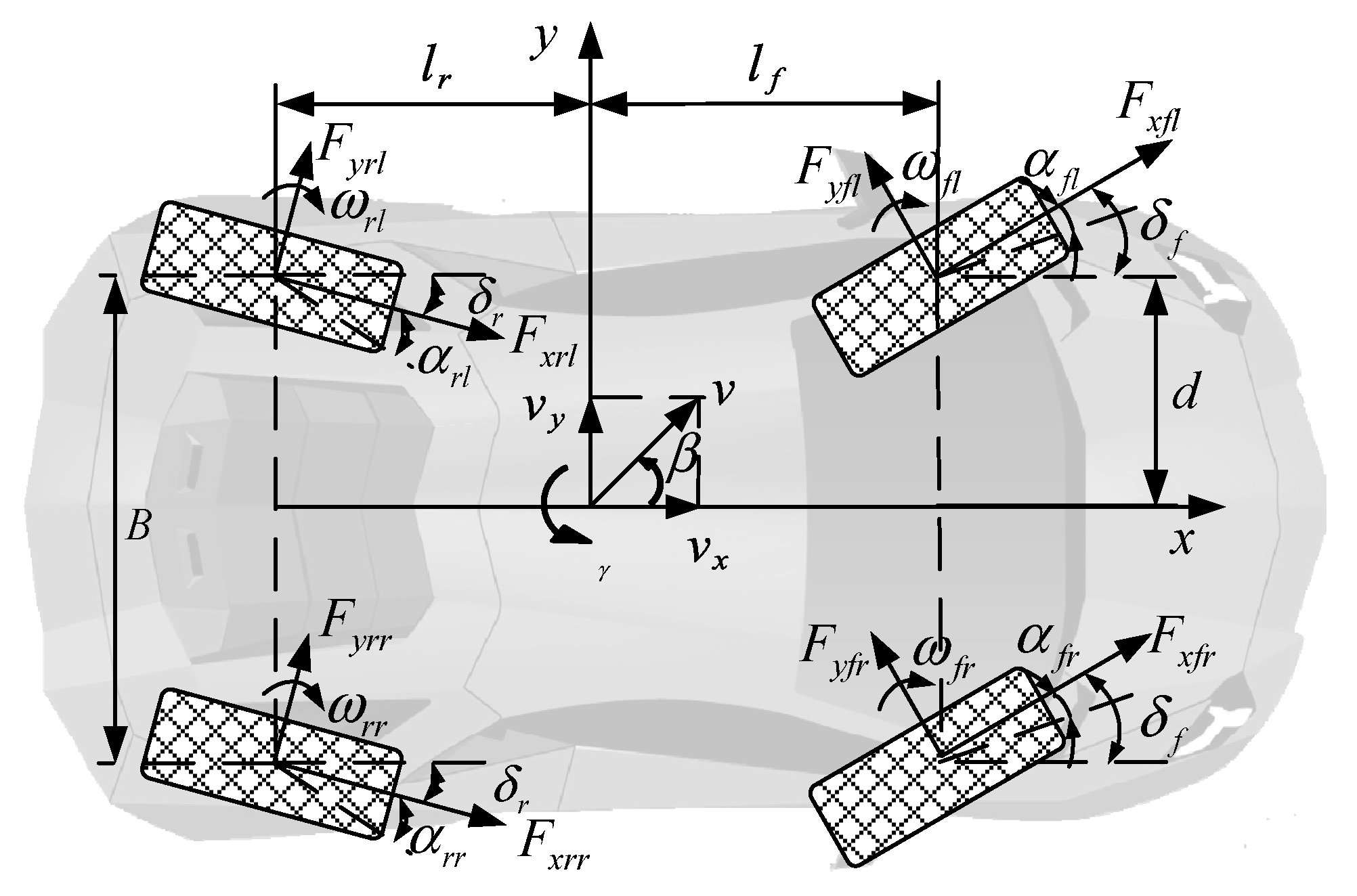
2.1. Nonlinear 7 DOF Model of Four-Wheel Steering

Assuming identical steering angles for both the left and right wheels on both the front and rear axles, as well as similar mechanical properties for all four tires, this model primarily takes into account the longitudinal, lateral, yaw, and rotational motions of the four wheels. As illustrated in Figure 1, the nonlinear 7 DOF model is utilized to represent the 4WS system in DDEVs [15]. Additionally, Figure 2 displays the wheel rotation model, which is employed to describe the rotational movements of each wheel.

The longitudinal dynamics can be represented as follows:

$$\begin{array}{cc}\hfill m({\dot{v}}_x-\gamma v_y)& =(F_{xfl}+F_{xfr})\cos {\delta }_f\hfill \\ & -(F_{yfl}+F_{yfr})\sin {\delta }_f\hfill \\ & +(F_{xrl}+F_{xrr})\cos {\delta }_r\hfill \\ & -(F_{yrl}+F_{yrr})\sin {\delta }_r\hfill \end{array}$$

(1)

The lateral dynamics can be described as follows:

$$\begin{array}{cc}\hfill m({\dot{v}}_y+\gamma v_x)& =(F_{xfl}+F_{xfr})\sin {\delta }_f\hfill \\ & +(F_{yfl}+F_{yfr})\cos {\delta }_f\hfill \\ & +(F_{xrl}+F_{xrr})\sin {\delta }_r\hfill \\ & +(F_{yrl}+F_{yrr})\cos {\delta }_r\hfill \end{array}$$

(2)

The yaw motion of the vehicle body can be described as follows:

$$\begin{array}{cc}\hfill I_z\stackrel{•}{\gamma }& =[(F_{xfl}+F_{xfr})\sin {\delta }_f+(F_{yfl}+F_{yfr})\cos {\delta }_f]l_f\hfill \\ & +[(F_{xfr}-F_{xfl})\cos {\delta }_f+(F_{yfl}-F_{yfr})\sin {\delta }_f]d\hfill \\ & -[(F_{xrl}+F_{xrr})\sin {\delta }_r+(F_{yrl}+F_{yrr})\cos {\delta }_r]l_r\hfill \\ & +[(F_{xrr}-F_{xrl})\cos {\delta }_r+(F_{yrl}-F_{yrr})\sin {\delta }_r]d\hfill \end{array}$$

(3)

where $l_f$ and $l_r$ are the distances from the center of gravity to the front and rear axles, respectively; $d=B/2$ is half of the track width; ${\delta }_f$ and ${\delta }_r$ are the front and rear wheel steering angles, respectively; $m$ is the vehicle mass; $v_x$ and $v_y$ are the vehicle longitudinal speed and lateral speed, respectively; $I_z$ is the vehicle yaw moment of inertia; $F_{xij}$ and $F_{yij}$ are the longitudinal and lateral forces of the four wheels, respectively (where $ij=fl,fr,rl,rr$, denoting the front left, front right, rear left, and rear right wheels); and $\gamma$ is the yaw rate.

The wheels’ rotational motions can be expressed as follows:

$$I_{\omega ij}·{\dot{\omega }}_{ij}=T_{dij}-T_{bij}-T_{fij}-R_{wij}{F}_{xij}$$

(4)

The vertical force of the tire can be described as follows:

$$\left\{\begin{array}{l}{F}_{zfl}=mg\frac{l_r}{2L}-m{a}_x\frac{h_g}{2L}-m{a}_y\frac{h_g}{2d_f}\frac{l_r}{L}\\ F_{zfr}=mg\frac{l_r}{2L}-m{a}_x\frac{h_g}{2L}+m{a}_y\frac{h_g}{2d_f}\frac{l_r}{L}\\ F_{zrl}=mg\frac{l_f}{2L}+m{a}_x\frac{h_g}{2L}-m{a}_y\frac{h_g}{2d_r}\frac{l_f}{L}\\ F_{zrr}=mg\frac{l_f}{2L}+m{a}_x\frac{h_g}{2L}+m{a}_y\frac{h_g}{2d_r}\frac{l_f}{L}\end{array}\right.$$

(5)

where $T_{dij}$, $T_{bij}$, and $T_{fij}$ are the driving torque, the brake torque, and the rolling resistance torque of each wheel, respectively; ${\omega }_{ij}$ is the wheel angular acceleration; $I_{\omega ij}$ is the wheel inertia moment; $a_x={\dot{v}}_x-\gamma v_y$ and $a_y={\dot{v}}_y+\gamma v_x$ are the longitudinal and lateral accelerations, respectively; $L=l_r+l_f$ is the wheelbase; $R_{wij}$ is the radius of each wheel; and $h_g$ is the height of the gravity center.

2.2. Tire Model

Tires play an important role in vehicle dynamics due to the mechanical properties of complex nonlinearity. The magic formula (MF) is adopted to describe the tire characteristics. The general calculation procedure can be represented as follows:

$$y=D\sin \left\{\begin{array}{l}C\arctan [B(x+S_H)\\ -E\left(B(x+S_H)-\arctan \left(B(x+S_H)\right)\right)]\end{array}\right\}+S_V$$

(6)

where $D$, $C$, $B$, and $E$ are the peak factor, the shape factor, the stiffness factor, and the curvature factor, respectively; $S_H$ and $S_V$ are the horizontal and vertical offsets of the tire force, respectively; $y$ represents the longitudinal or lateral force; and $x$ represents the longitudinal slip ratio or the tire sideslip angle, which are defined as follows:

$${\lambda }_{ij}=\left\{\begin{array}{l}\frac{{\omega }_{ij}{R}_{wij}-v_{xwij}}{{\omega }_{ij}{R}_{wij}} {\omega }_{ij}{R}_{wij}\ge v_{xwij} \mathrm{acceleration}\\ \frac{v_{xwij}-{\omega }_{ij}{R}_{wij}}{v_{xwij}} {\omega }_{ij}{R}_{wij}<v_{xwij} \mathrm{braking}\end{array}\right.$$

(7)

$$\left\{\begin{array}{l}{\alpha }_{fl}=\arctan (\frac{v_y+l_f\gamma }{v_x-d\gamma })-{\delta }_f\\ {\alpha }_{fr}=\arctan (\frac{v_y+l_f\gamma }{v_x+d\gamma })-{\delta }_f\\ {\alpha }_{rl}=\arctan (\frac{v_y-l_r\gamma }{v_x-d\gamma })-{\delta }_r\\ {\alpha }_{rr}=\arctan (\frac{v_y-l_r\gamma }{v_x+d\gamma })-{\delta }_r\end{array}\right.$$

(8)

where $v_{xwij}$ is the longitudinal speed of the wheel center.

With the assumption that the tire slip angle is much smaller, the tire force has a linear relationship with respect to the tire slip angle.

$$\left\{\begin{array}{l}{F}_{yf}=K_f{\alpha }_f\\ F_{yr}=K_r{\alpha }_r\end{array}\right.$$

(9)

where $K_f$ and $K_r$ are the cornering stiffnesses of the front and rear tires.

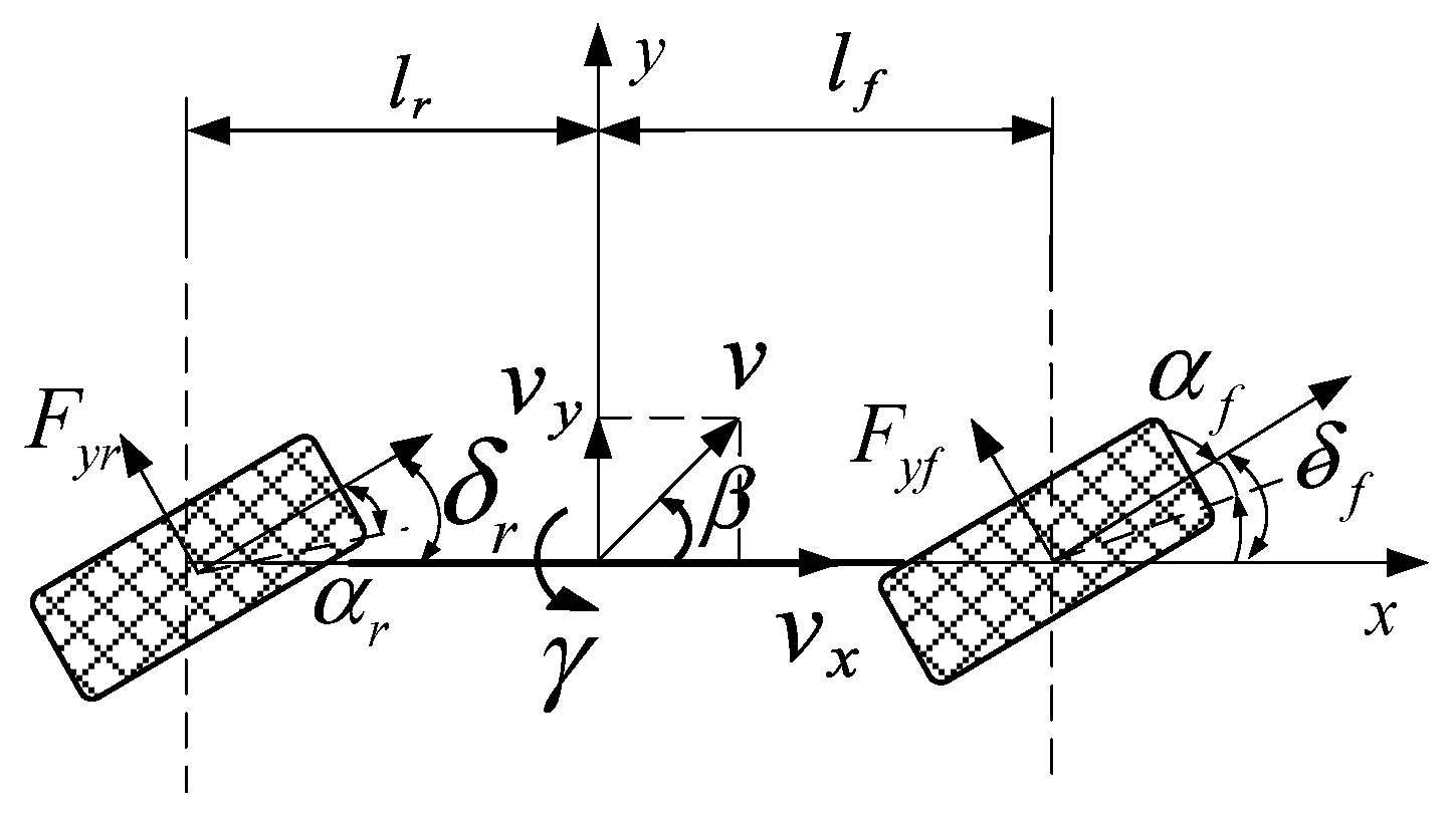
2.3. Linear 2-DOF Model of Four-Wheel Steering

To reduce the modeling complexity, a linear 2-DOF reference model for a vehicle with a 4WS system is necessary in order to design the optimal yaw motion and to obtain the reference yaw rate and sideslip angle for the controller [15]. It is assumed that the vehicle travels at a constant speed on a level road surface. When the angle is small enough, the motion depicted in Figure 3 could be depicted as follows:

$$\left\{\begin{array}{l}m{v}_x(\dot{\beta }+\gamma )=F_{yr}+F_{yf}\\ I_z\dot{\gamma }=F_{yf}{l}_f-F_{yr}{l}_r\end{array}\right.$$

(10)

where $\beta$ is the sideslip angle of the mass center; and $F_{yf}$ and $F_{yr}$ are the lateral forces of the front and rear tires, respectively.

Since $v_x$ is regarded as a constant value, with the substitution of (8) and (9) into (10), the linear dynamical equations of the single-track model could be written as follows:

$$\begin{array}{cc}\hfill \left[\begin{array}{l}\dot{\beta }\\ \dot{\gamma }\end{array}\right]& =\left[\begin{array}{cc}\frac{K_f+K_r}{m{v}_x}& \frac{l_f{K}_f-l_r{K}_r}{m{v_x}^2}-1\\ \frac{l_f{K}_f-l_r{K}_r}{I_z}& \frac{{l_f}^2{K}_f+{l_r}^2{K}_r}{I_z{v}_x}\end{array}\right]\left[\begin{array}{l}\beta \\ \gamma \end{array}\right]\hfill \\ & +\left[\begin{array}{cc}\frac{-K_f}{m{v}_x}& \frac{-K_r}{m{v}_x}\\ \frac{-l_f{K}_f}{I_z}& \frac{l_r{K}_r}{I_z}\end{array}\right]\left[\begin{array}{l}{\delta }_f\\ {\delta }_r\end{array}\right]\hfill \end{array}$$

(11)

When the DDEVs enter the steady state, the reference model of the sideslip angle and yaw rate is represented as follows:

$$\begin{array}{l}{\beta }_d=\frac{l_r+\frac{l_{f}m{v_x}^2}{L{K}_r}}{L(1+K{v_x}^2)}{\delta }_f+\frac{l_f-\frac{l_{r}m{v_x}^2}{L{K}_f}}{L(1+K{v_x}^2)}{\delta }_r,\\ {\gamma }_d=\frac{v_x}{L(1+K{v_x}^2)}({\delta }_f-{\delta }_r)\end{array}$$

(12)

where $K=\frac{m}{L^2}·\frac{l_f{K}_f-l_r{K}_r}{K_f{K}_r}$ is the stability factor.

3. Phase Plane Analysis

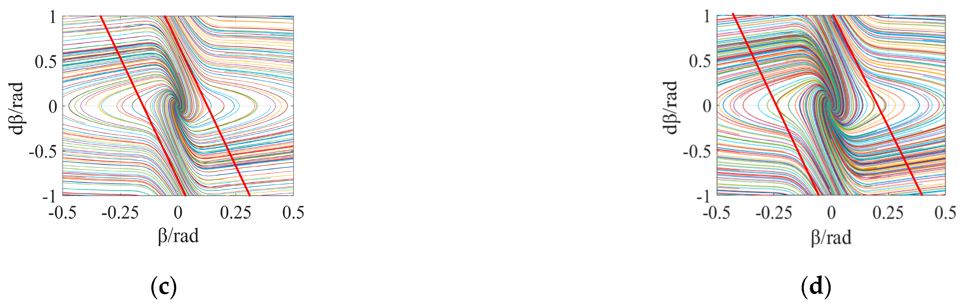
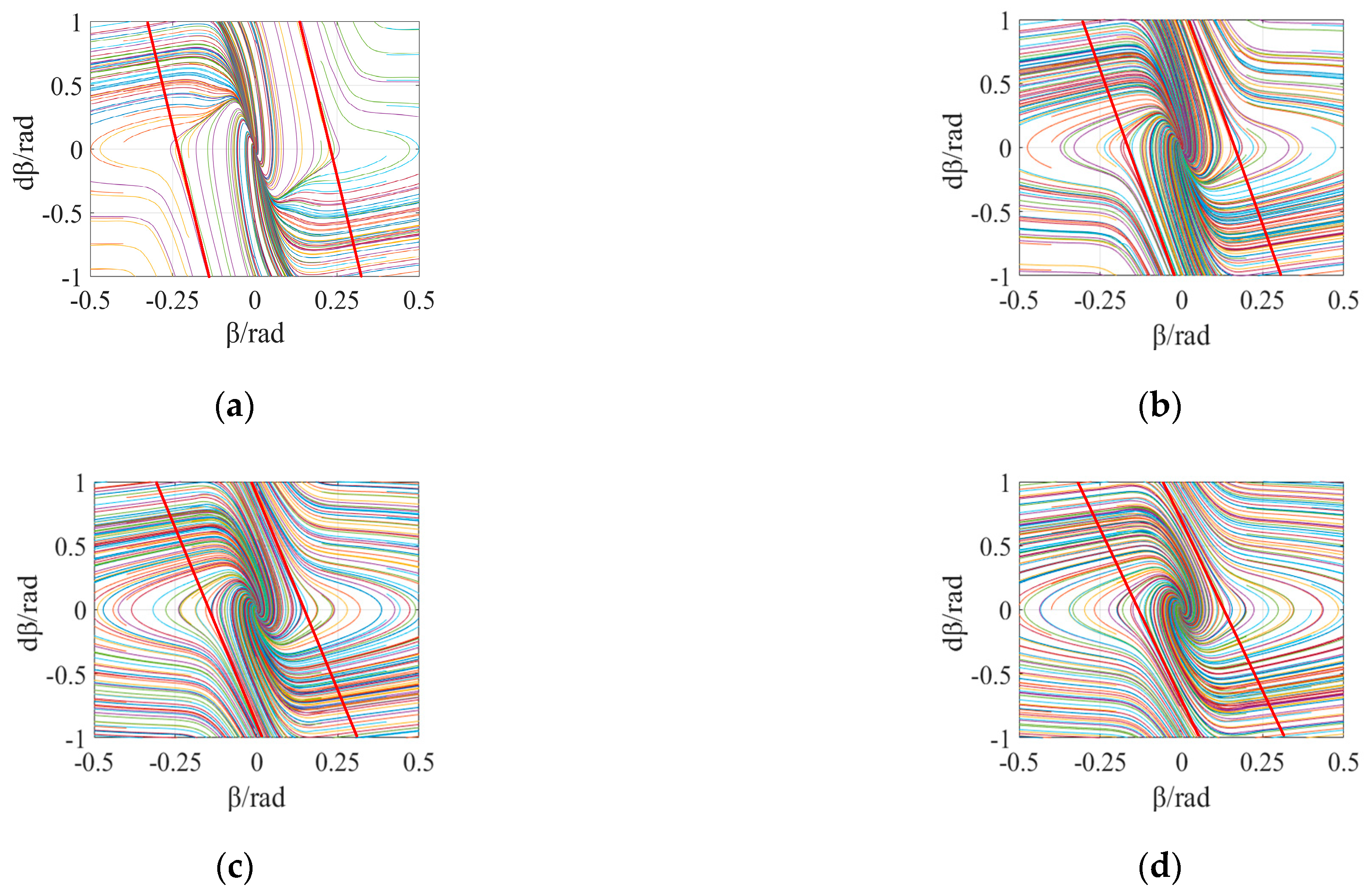
3.1. Phase Plane Stable Region Division

Phase plane methodology is a powerful tool for qualitatively describing and analyzing the stability of 4WS vehicles, with the $\beta -\dot{\beta }$ phase plane and $\beta -\gamma$ phase plane being the most commonly used. By analyzing the phase trajectory, the phase plane can provide an intuitive analysis of the stable state, the equilibrium position, and the effect of specific parameters on the vehicle stability. Phase plane methodology suggests the existence of a linear strip region in which all phase trajectories finally converge to a stable point. The yaw rate and sideslip angle are two crucial values that can reflect the stability of DDEVs. This paper adopts the $\beta -\dot{\beta }$ phase plane due to its mathematical simplicity and sensitivity to key factors such as the longitudinal speed, road adhesion coefficient, and front and rear wheel steering angles.

The strip region can be displayed by the boundaries of the stable region. To accurately determine the stable region of 4WS vehicles in the phase plane, it is necessary to modify the conventional two-line method applied to front-wheel steering vehicles. This is because the dynamics of a 4WS system are more complex and involve additional parameters that affect stability. Therefore, in this study, a modified two-line method is proposed to investigate the impact of the longitudinal speed, road adhesion coefficient, and front and rear wheel steering angles on the stable region in the $\beta -\dot{\beta }$ phase plane. The boundaries of the stable region can be mathematically expressed based on this approach.

$$\left\{\begin{array}{c}{E}_1\beta +\dot{\beta }=E_2\\ E_1\beta +\dot{\beta }=E_3\end{array}\right.$$

(13)

where $E_1$ is the slope of the upper and lower boundaries of the stability region and $E_2$ and $E_3$ are the intercepts of the upper and lower boundaries of the stability region, respectively.

Figure 4 illustrates the impact of varying front and rear wheel steering angles on the $\beta -\dot{\beta }$ phase plane when the longitudinal speed of $v_x=60\mathrm{km}/\mathrm{h}$ and the road adhesion coefficient of $\mu =0.8$ are constant. It could be observed that, as the steering angle increases, the stable region shifts towards the horizontal axis. Therefore, it is assumed that the front and rear wheel steering angles affect only $E_2$ and $E_3$ but not $E_1$. Figure 4a,b show that, when the steering angle of the front wheel is increased, the stable region’s size remains basically unchanged, but the stable point and strip region shift. Similarly, Figure 4c,d indicate that the stable point is far away from the origin and the strip region shifts accordingly when the steering angle of the rear wheel increases. Figure 4e,f show that the stable point of the phase plane shifts on the horizontal axis when the front and rear wheels steer in the same direction, with the stable point leaving further away from the origin of the axes as the steering angle increases. However, the stable region of the phase plane remains symmetric about the stable point when the front and rear wheel steering angles are the same. Figure 4g,h indicate that, when the front-wheel steering and rear-wheel steering are in opposite directions, the stable point of the phase plane shifts on the horizontal axis, and the stable region changes. Here, the reference sideslip angle of the mass center is not zero, and, as the steering angles increase, the stable point moves further away from the origin of the axes. It could be observed, when reverse rear-wheel steering is added to the front-wheel steering, the range of the stable region may be reduced, and the stable point may even disappear, indicating a reduction in the DDEVs’ stability margin and leading to vehicle instability. Additionally, when the front and rear wheel steering angles differ, the phase plane stable region boundaries may no longer be parallel, but the impact of the wheel steering angles on the slope of the boundaries is limited and can be neglected in stability boundary modeling.

Figure 5 illustrates the effect of the road adhesion coefficient on the $\beta -\dot{\beta }$ phase plane when the longitudinal speed of $v_x=80\mathrm{km}/\mathrm{h}$ and the front and rear wheel steering angles of ${\delta }_f=0,{\delta }_r=0$ are constant. With the road adhesion coefficient increasing, the size of the stable region extends by degrees, while the strip region remains unaffected with no offsets. This indicates that the road adhesion coefficient has little influence on the slope of the stability boundaries but significantly affects the size of the stable region. Thus, it can be inferred that this road adhesion coefficient exerts a significant influence on $E_2$ and $E_3$. Moreover, the stable point of the phase plane is located at the origin of the coordinates, and the boundaries of the stable region are symmetric about the origin. Figure 5a,b reveal that, on low-adhesion roads, the range of the stable region is very narrow, and parts of the phase tracks fail to converge to the stable point, indicating that the DDEV is prone to instability and difficult to control. Conversely, high-adhesion roads offer better maximum adhesion, resulting in a larger vehicle stability margin.

Figure 6 illustrates the impact of the longitudinal vehicle speed on the $\beta -\dot{\beta }$ phase plane when the road adhesion coefficient of $\mu =0.8$ and the front and rear wheel steering angles of ${\delta }_f=0,{\delta }_r=0$ are constant. As the speed increases, the size of the stable region decreases. Furthermore, the slope of the stability boundaries is heavily influenced by the longitudinal speed, indicating a correlation between $E_1$ and the vehicle speed. The stable point of the phase plane is situated at the origin of the coordinates, and the boundaries of the stable region are symmetric with respect to the origin.

3.2. Stability Boundary Model

To establish a steady-state boundary model of DDEVs at different speeds, the road adhesion coefficients, front and rear wheel angles, and stability boundary coefficients of the modified two-line method can be determined using polynomial fitting. When the longitudinal speed of $v_x=60\mathrm{km}/\mathrm{h}$ and the road adhesion coefficient of $\mu =0.8$ are constant, the vehicle’s front and rear steering angles are discretized into 13 data points with intervals of 3 degrees, within a range of −6 to 6 degrees. The boundary coefficients can be obtained for the various steering angles of the front and rear wheels, as presented in

Table 1. Boundary coefficients under different steering angles of the front and rear wheels.

${\mathit{\delta }}_{\mathit{f}},{\mathit{\delta }}_{\mathit{r}}$	${\mathit{E}}_2$	${\mathit{E}}_3$
6, 6	1.970	−0.552
6, 3	1.973	−0.490
3, 6	1.682	−0.938
3, 3	1.573	−0.816
3, 0	1.502	−0.936
0, 3	1.198	−1.219
0, 0	1.217	−1.217
0, −3	1.308	−1.213
−3, 0	0.936	−1.502
−3, −3	0.931	−1.629
−6, −3	0.497	−1.973
−3, −6	0.823	−1.641
−6, −6	0.447	−1.970

.

The intercept coefficients $E_2$ and $E_3$ of the stability boundary by using the polynomial fitting method can be given as follows:

$$\left\{\begin{array}{cc}\hfill E_2({\delta }_f,{\delta }_r)& =-1.045\times {10}^{-3}{\delta }_f^2+0.096{\delta }_f+1.304\times {10}^{-3}{\delta }_f{\delta }_r\hfill \\ & -3.268\times {10}^{-3}{\delta }_r^2+1.177\times {10}^{-2}{\delta }_r-1.179\hfill \\ \hfill E_3({\delta }_f,{\delta }_r)& =-1.181\times {10}^{-3}{\delta }_f^2+0.098{\delta }_f+0.877\times {10}^{-3}{\delta }_f{\delta }_r\hfill \\ & -1.592\times {10}^{-3}{\delta }_r^2+1.682\times {10}^{-2}{\delta }_r+1.225\hfill \end{array}\right.$$

(14)

The data fitting results of the boundary coefficients under different steering angles of the front and rear wheels are displayed in Figure 7.

To design a stability boundary model of DDEVs under different road adhesion coefficients, the road adhesion coefficient is discretized into seven data points with intervals of 0.1 within a range of 0.2~0.8 when the longitudinal speed of $v_x=80\mathrm{km}/\mathrm{h}$ and the front and rear wheel steering angles of ${\delta }_f=0,{\delta }_r=0$ are constant. By considering various road adhesion coefficients, the corresponding values of the boundary coefficients can be obtained and are presented in

Table 2. Boundary coefficients under different road adhesion coefficients.

$\mathit{\mu }$	${\mathit{E}}_2$	${\mathit{E}}_3$
0.2	0.241	−0.241
0.3	0.445	−0.445
0.4	0.588	−0.588
0.5	0.711	−0.711
0.6	0.878	−0.878
0.7	1.109	−1.109
0.8	1.217	−1.217

.

The intercept coefficients $E_2$ and $E_3$ of the stability boundary by using the polynomial fitting method can be given as follows:

$$\left\{\begin{array}{l}{E}_2(\mu )=0.022{\mu }^2+1.64\mu +0.084\\ E_3(\mu )=-0.022{\mu }^2-1.64\mu -0.084\end{array}\right.$$

(15)

To capture the effect of various longitudinal vehicle speeds on the stability boundaries, the vehicle speed range of 40~120 km/h is divided into nine data points with intervals of 10 km/h when the road adhesion coefficient of $\mu =0.8$ and the front and rear wheel steering angles of ${\delta }_f=0,{\delta }_r=0$ are constant. By varying the longitudinal vehicle speed, the corresponding boundary coefficients for each speed point can be obtained and are presented in

Table 3. Boundary coefficients at different longitudinal vehicle speeds.

${\mathit{v}}_{\mathit{x}}$	${\mathit{E}}_1$
120	−4.608
110	−4.950
100	−5.205
90	−5.329
80	−5.647
70	−5.935
60	−6.297
50	−6.785
40	−7.342

.

The slope coefficient $E_1$ of the stability boundary by using the polynomial fitting method can be given as follows:

$$E_1(v_x)=4.866\times {10}^{-6}{v_x}^3-1.388\times {10}^{-3}{v_x}^2+0.1549v_x-11.64$$

(16)

By combining the polynomial fitting results of the different road adhesion coefficients and steering angles with no coupling effect relationship between them, the boundary intercept can be expressed as follows:

$$\left\{\begin{array}{l}{E}_2=\frac{1}{2}[E_2({\delta }_f,{\delta }_r)+E_2(\mu )]\\ E_3=\frac{1}{2}[E_3({\delta }_f,{\delta }_r)+E_3(\mu )]\end{array}\right.$$

(17)

In the $\beta -\dot{\beta }$ phase plane, the state points are in the stable region when Equation (13), considering the stability boundary, is satisfied, which indicates that the DDEVs are in stable states. To define the stability or instability degree, this paper uses the vehicle stable-state coefficient $\kappa$ to represent the stable or unstable vehicle state. The calculation equation is obtained as follows:

$$\kappa =\left|\frac{E_2+E_3-2(E_1\beta +\dot{\beta })}{E_2-E_3}\right|$$

(18)

This vehicle stable-state coefficient is used to modify the weight matrix in the subsequent handling stability controller design. When $\kappa >1$ is satisfied, the vehicle is instable, and a larger coefficient value represents more serious instability of the vehicle; when $0<\kappa <1$ is satisfied, the vehicle is stable.

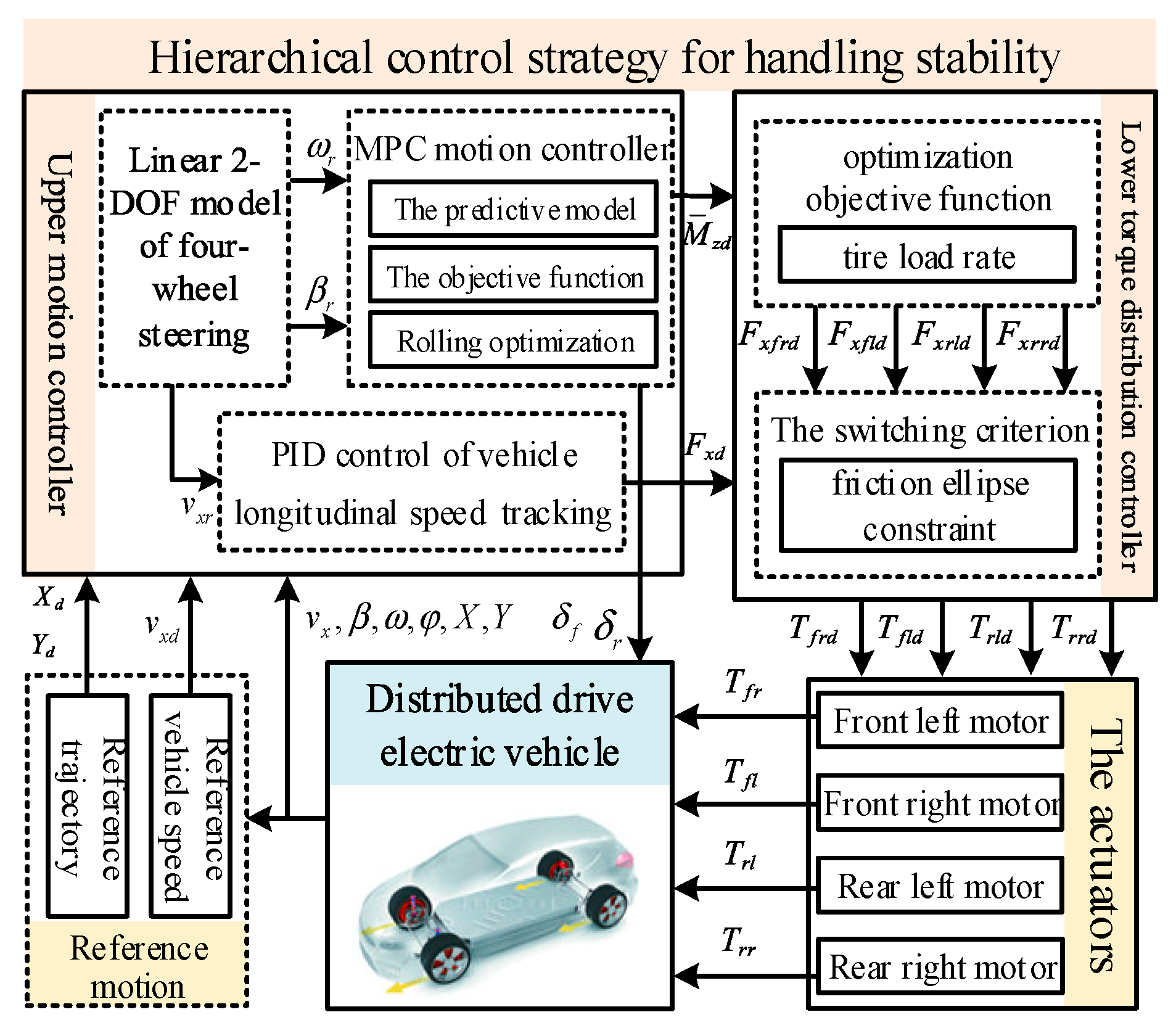
4. Hierarchical Stability Control Design

4.1. Control System Framework

This section provides a detailed explanation of the hierarchical handling stability control, which follows a two-layer framework. The upper layer utilizes a model predictive controller to track the reference states, while the lower layer employs a modified distribution algorithm to reconfigure the control quantities of the actuators. The control system’s framework is illustrated in Figure 8.

The presented control system consists of a hierarchical two-layer framework, where the upper layer utilizes the reference output layer to generate target values for the longitudinal traction, yaw moment control, and tracking control of the reference trajectory, achieving an integrated control. However, the lower layer is implemented based on a two-level optimal distribution control algorithm, which aims to minimize the tire load rate to ensure the maximum vehicle stability margin. By employing the friction ellipse constraint, the lower layer controller distributes the generalized control force from the upper layer controller to the four wheel motors in the form of torque commands.

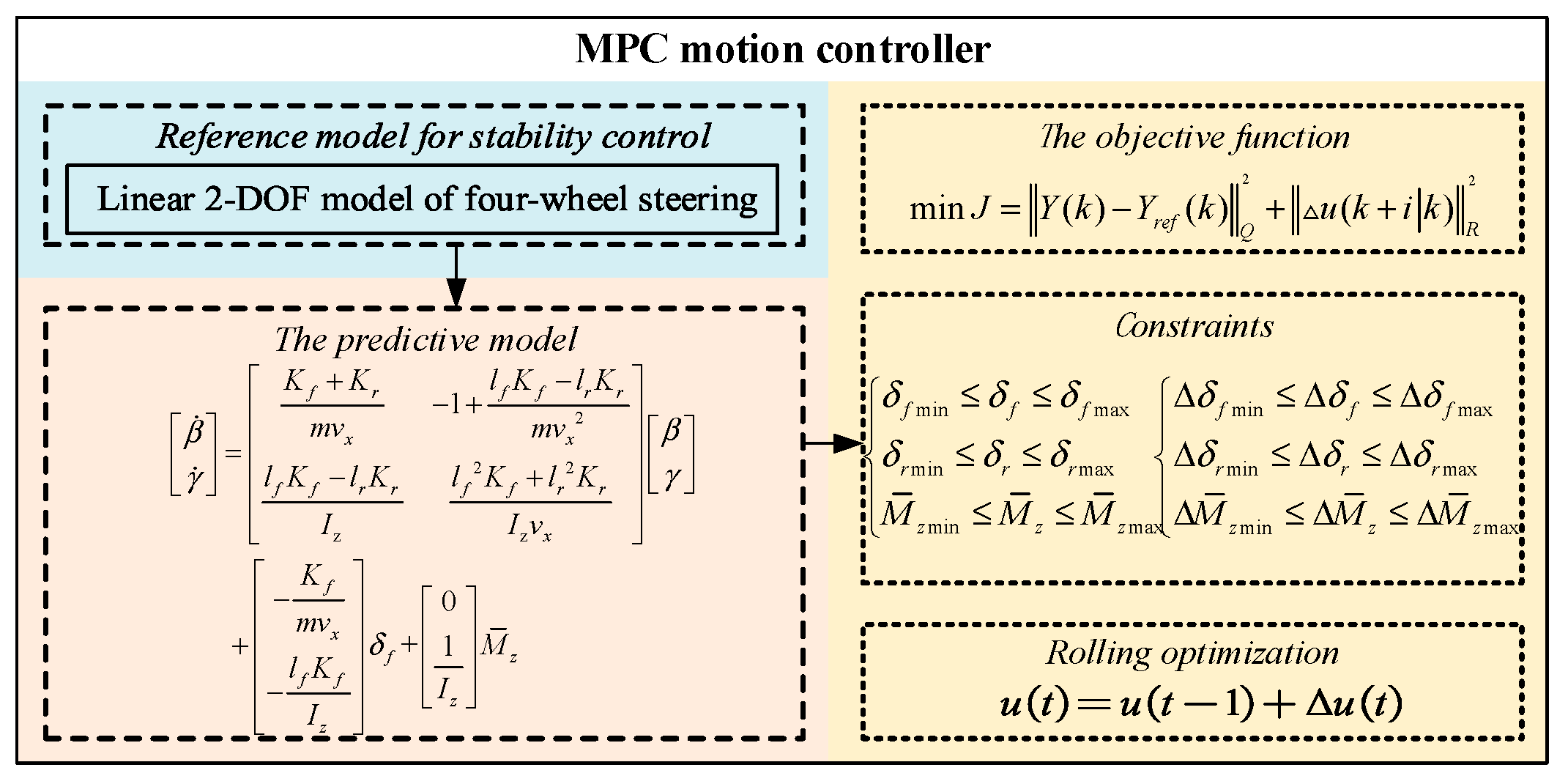
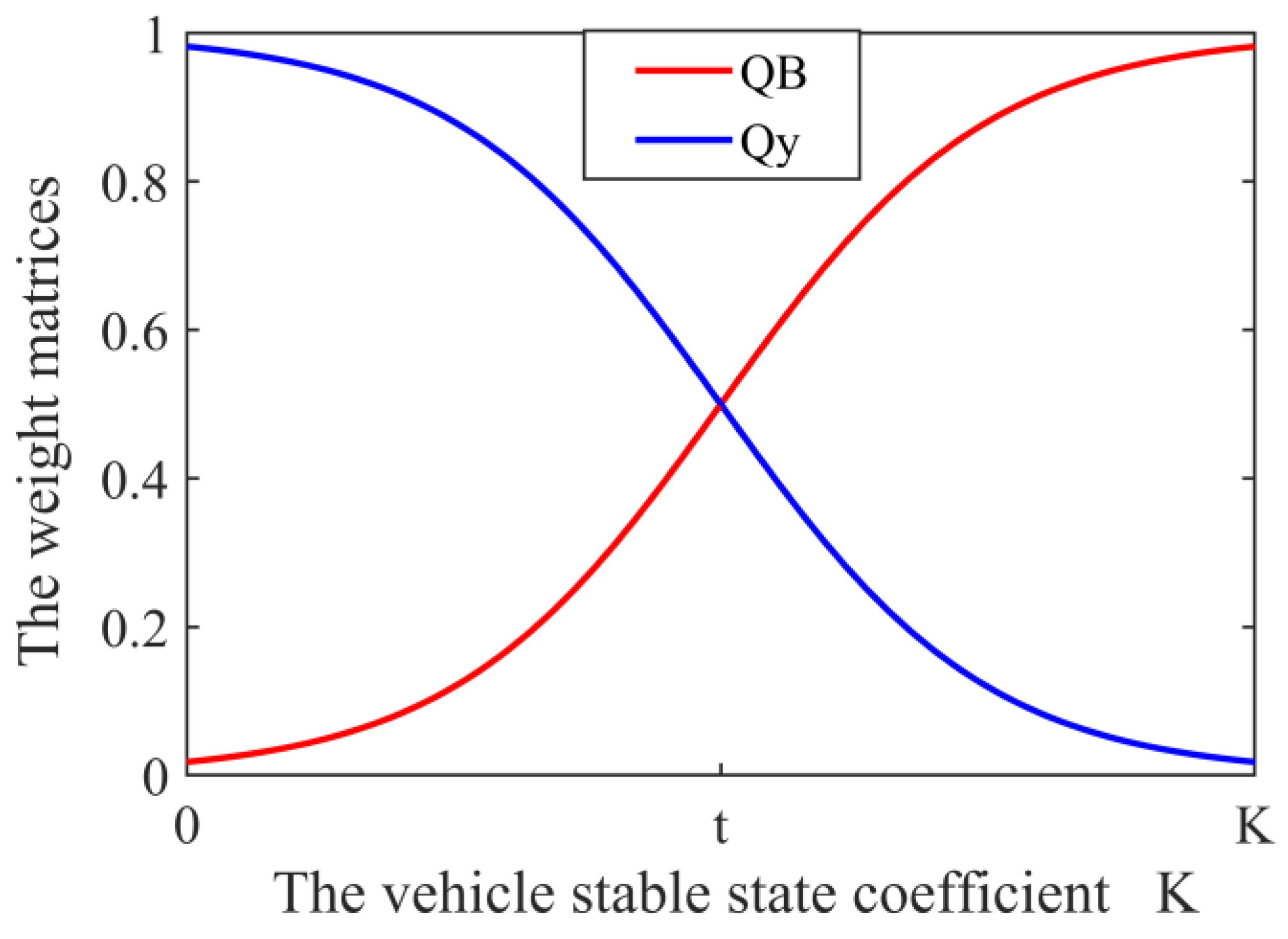
4.2. Upper Motion Controller

In order to accomplish motion tracking control, the control of both longitudinal and lateral dynamics is needed. While the MPC controller is introduced into the yaw moment control, a simple PID controller can achieve the longitudinal traction. To make the real longitudinal speed $v_x$ close to the reference longitudinal speed $v_{xd}$, via adjusting the longitudinal force $F_{xd}$, the PID controller is designed to track the desired vehicle speed, which is based on the deviation between the actual speed $v_x\left(t\right)$ and the expected speed $v_{xd}\left(t\right)$.

The linear 2-DOF model of 4WS is utilized to calculate the parameters of the reference yaw rate ${\gamma }_d$ and the reference sideslip angle ${\beta }_d$. Based on this reference model, the MPC motion controller generates the expected yaw moment by taking into account the desired sideslip angle ${\beta }_d$ and yaw rate ${\gamma }_d$. The design of an MPC controller typically involves three main components, namely, the selection of a predictive model, the construction of the objective function, and the computation of the optimal control sequence. A schematic of the framework of the MPC motion controller is presented in Figure 9.

Considering the influence of the additional yaw moment ${\overline{M}}_Z$ on the state control in the DYC control system, it is brought into the 2-DOF model of four-wheel steering as a control variable to obtain the following expression:

$$\left\{\begin{array}{l}m{v}_x(\dot{\beta }+\gamma )=F_{yr}\cos {\delta }_r+F_{yf}\cos {\delta }_f\\ I_z\dot{\gamma }=F_{yf}{l}_f\cos {\delta }_f-F_{yr}{l}_r\cos {\delta }_r+{\overline{M}}_Z\end{array}\right.$$

(19)

Then, the following prediction model state equation can be established as follows:

$$\begin{array}{cc}\hfill \left[\begin{array}{c}\dot{\beta }\\ \dot{\gamma }\end{array}\right]& =\left[\begin{array}{cc}\frac{K_f+K_r}{m{v}_x}& -1+\frac{l_f{K}_f-l_r{K}_r}{m{v_x}^2}\\ \frac{l_f{K}_f-l_r{K}_r}{I_{\mathrm{z}}}& \frac{{l_f}^2{K}_f+{l_r}^2{K}_r}{I_{\mathrm{z}}{v}_x}\end{array}\right]\left[\begin{array}{c}\beta \\ \gamma \end{array}\right]\hfill \\ & +\left[\begin{array}{cc}-\frac{K_f}{m{v}_x}& -\frac{K_r}{m{v}_x}\\ -\frac{l_f{K}_f}{I_z}& \frac{l_r{K}_r}{I_z}\end{array}\right]\left[\begin{array}{l}{\delta }_f\\ {\delta }_r\end{array}\right]+\left[\begin{array}{c}0\\ \frac{1}{I_z}\end{array}\right]{\overline{M}}_z\hfill \end{array}$$

(20)

Equation (20) is converted into a state space representation as follows:

$$\begin{array}{c}\left\{\begin{array}{l}\dot{X}=A_{1}X+B_{1}U\\ Y=C_{1}X+D_{1}U\end{array}\right.\\ A_1=\left[\begin{array}{cc}\frac{K_f+K_r}{m{v}_x}& -1+\frac{l_f{K}_f-l_r{K}_r}{m{v_x}^2}\\ \frac{l_f{K}_f-l_r{K}_r}{I_{\mathrm{z}}}& \frac{{l_f}^2{K}_f+{l_r}^2{K}_r}{I_{\mathrm{z}}{v}_x}\end{array}\right],C_1=\left[\begin{array}{cc}1& 0\\ 0& 1\end{array}\right],\\ B_1=\left[\begin{array}{ccc}-\frac{K_f}{m{v}_x}& -\frac{K_r}{m{v}_x}& 0\\ -\frac{l_f{K}_f}{I_z}& \frac{l_r{K}_r}{I_z}& \frac{1}{I_z}\end{array}\right],D_1=\left[\begin{array}{ccc}0& 0& 0\\ 0& 0& 0\end{array}\right]\end{array}$$

(21)

where $X={\left[\begin{array}{cc}\beta & \gamma \end{array}\right]}^T$ is the state vector; $U={\left[\begin{array}{ccc}{\delta }_f& {\delta }_r& {\overline{M}}_z\end{array}\right]}^T$ is the control input vector; and $A_1$, $B_1$, $C_1$, and $D_1$ are the coefficient matrices.

It is necessary to discretize the state equation and to establish a prediction model. The difference method is adopted, and the state space model can be expressed as follows:

$$\left\{\begin{array}{l}\Delta x(k+1)=A_k\Delta x(k)+B_k\Delta u(k)+D_k\Delta w(k)\\ y(k)=C_k\Delta x(k)+y(k-1)+E_{k}w(k)\end{array}\right.$$

(22)

where $A_k=I+A_{k-1}{T}_s$, $B_k=B_{k-1}{T}_s$, $C_k=C_{k-1}$, $D_k=D_{k-1}{T}_s$, and $E_k=E_{k-1}$.

Based on the known control quantities of the system, the MPC predicts the state of the system in a finite prediction time domain $N_p$ in the future and solves the optimal control quantity in the control time domain $N_c$. The state of the system in the prediction time domain $N_p$ can be expressed as follows:

$$\begin{array}{cc}\hfill \Delta x(k+1\left|k\right.)& =A_k\Delta x(k)+B_k\Delta u(k)+D_k\Delta w(k)\hfill \\ \hfill \Delta x(k+2\left|k\right.)& ={A_k}^2\Delta x(k)+A_k{B}_k\Delta u(k)+B_k\Delta u(k+1)+A_k{D}_k\Delta w(k)\hfill \\ & ⋮\hfill \\ \hfill \Delta x(k+N_c\left|k\right.)& ={A_k}^{N_c}\Delta x(k)+{A_k}^{N_c-1}{B}_k\Delta u(k)+{A_k}^{N_c-2}{B}_k\Delta u(k+1)\hfill \\ & +\dots +B_k\Delta u(k+N_c-1)+{A_k}^{N_c-1}{D}_k\Delta w(k)\hfill \\ & ⋮\hfill \\ \hfill \Delta x(k+N_p\left|k\right.)& ={A_k}^{N_p}\Delta x(k)+{A_k}^{N_p-1}{B}_k\Delta u(k)+{A_k}^{N_p-2}{B}_k\Delta u(k+1)\hfill \\ & +\dots +{A_k}^{N_p-N_C}{B}_k\Delta u(k+N_p-1)+{A_k}^{N_p-1}{D}_k\Delta w(k)\hfill \end{array}$$

(23)

The output of the system in the prediction time domain can be expressed as follows:

$$\begin{array}{cc}\hfill y(k+1\left|k\right.)& =C_k{A}_k\Delta x(k)+C_k{B}_k\Delta u(k)+C_k{D}_k\Delta w(k)+y(k-1)\hfill \\ \hfill y(k+2\left|k\right.)& =(C_k{A_k}^2+C_k{A}_k)\Delta x(k)+(C_k{A}_k{B}_k+C_k{B}_k)\Delta u(k)+\hfill \\ & C_k{B}_k\Delta u(k+1)+(C_k{A}_k{D}_k+C_k{D}_k)\Delta w(k)+y(k-1)\hfill \\ & ⋮\hfill \\ \hfill y(k+N_c\left|k\right.)& ={\displaystyle \sum _{i=1}^{N_c}{C}_k{A_k}^i\Delta x(k)}+{\displaystyle \sum _{i=1}^{N_c}{C}_k{A_k}^{i-1}{B}_k\Delta u(k)}+{\displaystyle \sum _{i=1}^{N_c}{C}_k{A_k}^{i-2}{B}_k\Delta u(k+1)}\hfill \\ & +\dots +C_k{B}_k\Delta u(k+N_c-1)+{\displaystyle \sum _{i=1}^{N_c}{C}_k{A_k}^{i-1}{D}_k\Delta w(k)}+y(k-1)\hfill \\ & ⋮\hfill \\ \hfill y(k+N_p\left|k\right.)& ={\displaystyle \sum _{i=1}^{N_p}{C}_k{A_k}^i\Delta x(k)}+{\displaystyle \sum _{i=1}^{N_p}{C}_k{A_k}^{i-1}{B}_k\Delta u(k)}+{\displaystyle \sum _{i=1}^{N_p}{C}_k{A_k}^{i-2}{B}_k\Delta u(k+1)}\hfill \\ & +\dots +{\displaystyle \sum _{i=1}^{N_p-N_c+1}{C}_k{A_k}^{i-1}{B}_k\Delta u(k+N_p-1)}\hfill \\ & +{\displaystyle \sum _{i=1}^{N_p}{C}_k{A_k}^{i-1}{D}_k\Delta w(k)}+y(k-1)\hfill \end{array}$$

(24)

Based on the discretized system equation, the predictive output equation is constructed as follows:

$$Y(k)=S_X\Delta X(k)+S_W\Delta W(k)+S_U\Delta U(k)+Iy(k-1)$$

(25)

where $S_X=\left[\begin{array}{c}{C}_k{A}_k\\ {\displaystyle \sum _{i=1}^2{C}_k{A_k}^i}\\ ⋮\\ {\displaystyle \sum _{i=1}^{N_p}{C}_k{A_k}^i}\end{array}\right]$, $S_W=\left[\begin{array}{c}{C}_k{D}_k\\ {\displaystyle \sum _{i=1}^2{C}_k{A_k}^{i-1}{B}_k}\\ ⋮\\ {\displaystyle \sum _{i=1}^{N_p}{C}_k{A_k}^{i-1}{B}_k}\end{array}\right]$, $S_U=\left[\begin{array}{cccc}{C}_k{B}_k& 0& \dots & 0\\ {\displaystyle \sum _{i=1}^2{C}_k{A_k}^{i-1}{B}_k}& C_k{B}_k& \dots & 0\\ ⋮& ⋮& \ddots & 0\\ {\displaystyle \sum _{i=1}^{N_c}{C}_k{A_k}^{i-1}{B}_k}& {\displaystyle \sum _{i=1}^{N_c-1}{C}_k{A_k}^{i-1}{B}_k}& \dots & C_k{B}_k\\ ⋮& ⋮& \ddots & ⋮\\ {\displaystyle \sum _{i=1}^{N_p}{C}_k{A_k}^{i-1}{B}_k}& {\displaystyle \sum _{i=1}^{N_p-1}{C}_k{A_k}^{i-1}{B}_k}& \dots & {\displaystyle \sum _{i=1}^{N_p-N_c+1}{C}_k{A_k}^{i-1}{B}_k}\end{array}\right]$, $Y(k)={\left[\begin{array}{cccc}y(k+1\left|k\right.)& y(k+2\left|k\right.)& \dots & y(k+N_p\left|k\right.)\end{array}\right]}^T$, $\Delta U(k)={\left[\begin{array}{cccc}\Delta u(k+1\left|k\right.)& \Delta u(k+2\left|k\right.)& \dots & \Delta u(k+N_c\left|k\right.)\end{array}\right]}^T$.

To construct the objective function of the MPC, it is necessary to consider the constraints of the system. Specifically, in view of the limitations imposed by the road adhesion coefficient, the yaw rate of the DDEV is constrained to fall within a certain range of lateral acceleration. Additionally, when the tires are in close proximity to their saturation points, the yaw rate does not continue to grow, thereby bounding the actual yaw rate. This constraint can be expressed mathematically as a nonlinear inequality constraint.

$$-0.85\frac{\mu g}{v_x}\le \gamma \le 0.85\frac{\mu g}{v_x}$$

(26)

Considering the limitations of vehicle subsystem mechanical actuators and dynamic performance, the maximum and minimum properties are set as follows:

$$\left\{\begin{array}{l}{\delta }_{f\min }\le {\delta }_f\le {\delta }_{f\max }\\ {\delta }_{r\min }\le {\delta }_r\le {\delta }_{r\max }\\ {\overline{M}}_{z\min }\le {\overline{M}}_z\le {\overline{M}}_{z\max }\end{array}\right.$$

(27)

$$\left\{\begin{array}{l}\Delta {\delta }_{f\min }\le \Delta {\delta }_f\le \Delta {\delta }_{f\max }\\ \Delta {\delta }_{r\min }\le \Delta {\delta }_r\le \Delta {\delta }_{r\max }\\ \Delta {\overline{M}}_{z\min }\le \Delta {\overline{M}}_z\le \Delta {\overline{M}}_{z\max }\end{array}\right.$$

(28)

The objective function of the yaw rate and the sideslip angle is expressed as follows:

$$\begin{array}{cc}\hfill J_1& ={\displaystyle \sum _{i=1}^{N_P}}\left[{\left(\beta (k+i\left|k\right.)-{\beta }_r(k+i\left|k\right.)\right)}^2\right.Q_{\beta }\hfill \\ & +\left.{\left(\gamma (k+i\left|k\right.)-{\gamma }_r(k+i\left|k\right.)\right)}^2{Q}_{\gamma }\right]\hfill \\ & ={‖\beta (k+i\left|k\right.)-{\beta }_r(k+i\left|k\right.)‖}_{Q_{\beta }}^2\hfill \\ & +{‖\gamma (k+i\left|k\right.)-{\gamma }_r(k+i\left|k\right.)‖}_{Q_{\gamma }}^2\hfill \end{array}$$

(29)

where $Q_{\beta }$ represents the weight matrices of the sideslip angle and $Q_{\gamma }$ represents the weight matrices of the yaw rate.

Additionally, to consider the difference between the actual and the desired trajectory, the objective function of the control increment can be described as follows:

$$J_2={\displaystyle \sum _{i=1}^{N_c}\left[{(\Delta u(k+i\left|k\right.))}^{2}R\right]}={‖\Delta u(k+i\left|k\right.)‖}_R^2$$

(30)

Based on the reference trajectory, the lateral deviation and heading angle deviation can be selected as the state parameters in the objective function. Then, the objective function of the MPC can be described as follows:

$$\begin{array}{cc}\hfill \min J& ={‖Y(k)-Y_{ref}(k)‖}_Q^2+{‖\Delta u(k+i\left|k\right.)‖}_R^2\hfill \\ & ={‖S_X\Delta X(k)+S_W\Delta W(k)+S_U\Delta U(k)+Iy(k-1)-Y_{ref}(k)‖}_Q^2\hfill \\ & +{‖\Delta U(k)‖}_R^2\hfill \end{array}$$

(31)

The quadratic programming algorithm is adopted to solve this problem. In order to gain the optimal control quantity, this objective function can be transformed as follows:

$$\begin{array}{l}\min J=\frac{1}{2}{x}^{*T}H{x}^{*}+G^T{x}^{*}\\ x^{*}=\left[\begin{array}{l}\Delta U(k)\\ \epsilon \end{array}\right],H=\left[\begin{array}{cc}2({S_U}^{T}Q{S}_U+R)& 0\\ 0& \sigma \end{array}\right],\\ G^T=\left[\begin{array}{cc}2{\left[S_X\Delta X(k)+S_W\Delta W(k)+Iy(k-1)-Y_{ref}(k)\right]}^{T}Q{S}_U& 0\end{array}\right]\end{array}$$

(32)

To guarantee the vehicle’s stability and maneuverability, a relationship between the weight matrices $Q_{\beta }$ and $Q_{\gamma }$ is established. In situations where the sideslip angle and its rate of change are small, priority is given to controlling the yaw rate in order to ensure maneuverability. Conversely, when the sideslip angle or its rate of change is large, priority is given to controlling the sideslip angle in order to ensure stability. Additionally, the weight matrices $Q_{\beta }$ and $Q_{\gamma }$ are adjusted in real time based on the vehicle stable-state coefficient proposed in the phase plane analysis, as illustrated in Figure 10.

$$\left\{\begin{array}{l}{Q}_{\beta }=\frac{1}{1+e^{-s(\kappa -t)}}\\ Q_{\gamma }=1-\frac{1}{1+e^{-s(\kappa -t)}}\end{array}\right.$$

(33)

4.3. Lower Torque Distribution Controller

The mathematical equation ensuring that the tire force is distributed optimally to achieve the desired motion of the DDEVs is described as follows:

$$v=Bu$$

(34)

where $v={\left[\begin{array}{cc}{F}_{xd}& {\overline{M}}_{zd}\end{array}\right]}^T$ is the control generalized force; $B=\left[\begin{array}{cccc}\begin{array}{l}\cos {\delta }_f\\ l_f\sin {\delta }_f-d\cos {\delta }_f\end{array}& \begin{array}{l}\cos {\delta }_f\\ l_f\sin {\delta }_f+d\cos {\delta }_f\end{array}& \begin{array}{l}\cos {\delta }_r\\ -l_r\sin {\delta }_r-d\cos {\delta }_r\end{array}& \begin{array}{l}\cos {\delta }_r\\ -l_r\sin {\delta }_r+d\cos {\delta }_r\end{array}\end{array}\right]$ is the coefficient matrix; and $u={\left[\begin{array}{cccc}{F}_{xfl}& F_{xfr}& F_{xrl}& F_{xrr}\end{array}\right]}^T$ is the longitudinal force.

The road adhesion limitation constrains this tire longitudinal force in the form of a friction ellipse.

$$\sqrt{{F_{xij}}^2+{F_{yij}}^2}\le {\mu }_{ij}{F}_{zij}$$

(35)

Equation (35) demonstrates a nonlinear inequality constraint, which is dependent on both the longitudinal and lateral forces of the tire, with the latter being computationally expensive to calculate using the magic formula. This constraint serves as the switching criterion for the optimal distribution, which is used to determine whether the optimal solution obtained from the first-level distribution control ${u^{*}}_1$ satisfies the road adhesion constraints [30]. If not, the second-level distribution control ${u^{*}}_2$ is initiated to calculate the optimal results.

The tire load rate can be defined as follows:

$${\Upsilon }_{ij}=\frac{\sqrt{{F_{xij}}^2+{F_{yij}}^2}}{{\mu }_{ij}{F}_{zij}}$$

(36)

As shown in Equation (36), this tire force reserve represents a sufficient vehicle stability margin. The optimized objective function can be transformed from the tire load rate:

$$\begin{array}{l}{J}_{11}={\displaystyle \sum _{i=1}^4{h}_{ij}{F}_{xij}^2}\\ h_{ij}=\frac{1+{k_{ij}}^2}{{\mu }_{ij}^2{F}_{zij}^2},k_{ij}=\frac{F_{yij}}{F_{xij}}\end{array}$$

(37)

The first-level optimal distribution control can be written as follows:

$$\left\{\begin{array}{l}u=\arg \min J_{11}\\ s.t. u^{-}\le u\le u^{+}\end{array}\right.$$

(38)

The optimal solution of the tire longitudinal force ${u^{*}}_1$ can be carried out.

However, in real-world vehicle driving scenarios, the adhesion conditions of each wheel may not be uniform. If the simple addition of the tire load rate is adopted as the performance objective function, significant differences between the four wheels in the adhesion margin may arise. To address this issue, the weight coefficients are introduced, taking into account the varying adhesion conditions of each wheel during vehicle operation. This approach guarantees the maximum stability margin by providing the wheels with large adhesion margins under low-adhesion conditions. The objective function is formulated as follows:

$$J_{12}^{\prime }={‖{\Gamma }_{1}u‖}^2$$

(39)

where ${\psi }_{ij}=\frac{{\displaystyle \sum {\mu }_{ij}{F}_{zij}}}{{\mu }_{ij}{F}_{zij}}$ and ${\Gamma }_1=diag\left(\frac{{\psi }_{ij}}{{\mu }_{ij}{F}_{zij}}\right)$.

The objective function is converted into a standard form containing a cost function by introducing an error penalty.

$$J_{12}={‖{\Gamma }_{1}u‖}^2+\zeta {‖W_v\left(Bu-v\right)‖}^2$$

(40)

where $W_v$ is the control priority weight matrix and $\zeta$ is the penalty weight coefficient.

Then, the weight matrix $W_v$ is modified by the vehicle stable-state coefficient obtained in the phase plane analysis:

$$\begin{array}{l}{W}_v=diag\left({W_{Fd}/\kappa }^{*},{\kappa }^{*}{W}_{Mzd}\right)\\ {\kappa }^{*}=\left\{\begin{array}{cc}1& \kappa \le 1\\ \kappa & \kappa >1\end{array}\right.\end{array}$$

(41)

The second-level optimal distribution control can be written as follows:

$$\left\{\begin{array}{l}u=\arg \min J_{12}\\ =\arg \min ({‖{\Gamma }_{1}u‖}^2+\zeta {‖W_v\left(Bu-v\right)‖}^2)\\ s.t. u^{-}\le u\le u^{+}\end{array}\right.$$

(42)

The optimal solution of the tire longitudinal force ${u^{*}}_2$ can be carried out.

5. Simulation and Results

For the sake of verifying the feasibility of the established hierarchical control strategy, verification was carried out in a modeling simulation experiment. The simulation experiments were implemented by a CarSim and MATLAB/Simulink co-simulation to evaluate the control performance and reliability of the presented hierarchical handling stability control strategy for 4WS in comparison with those of other control strategies. The CarSim vehicle model was chosen as the controlled object, and the relevant vehicle parameters are presented in

Table 4. Vehicle model parameter table.

Vehicle Parameters	Value
Vehicle mass	1523 kg
Wheelbase	2.548 m
Distance from CG to front axle	1.163 m
Distance from CG to rear axle	1.385 m
Track width	1.530 m
Vehicle yaw moment of inertia	2023 kg·m3
Wheel inertia moment	0.95 kg·m3
Tire rolling radius	0.354 m
Frontal area	1.95 m2
Wind resistance coefficient	0.3
Height of CG	0.472 m

.

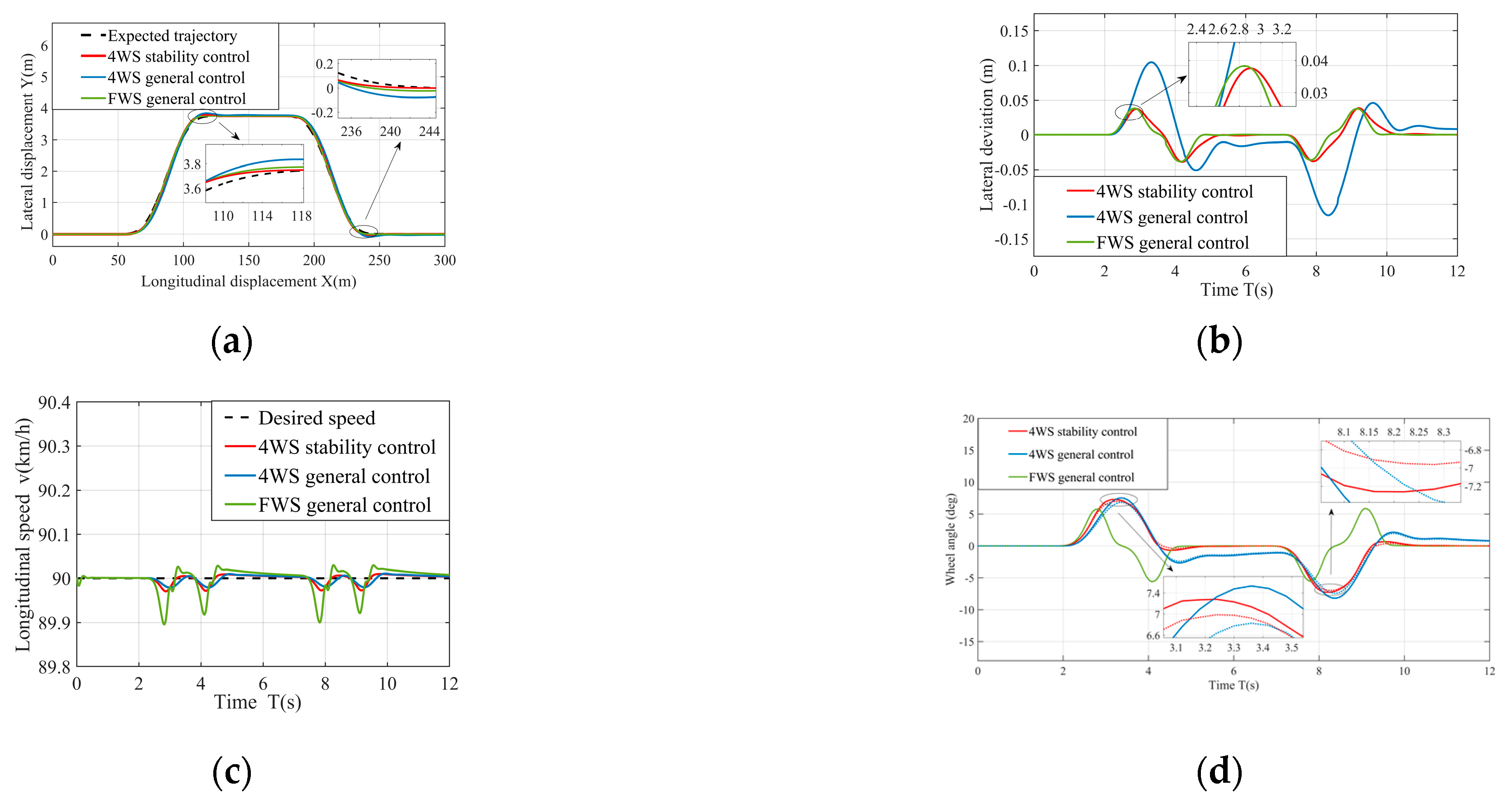
5.1. Double Lane Change Condition Simulation

To assess the handling stability of 4WS under a proposed hierarchical control strategy, a simulation of double lane change conditions was performed, with a comparison made with two other strategies: (1) The “4WS general control”, where its upper motion layer utilizes the MPC method to control the sideslip angle, yaw rate, and longitudinal speed without considering adjustments to the motion state reference properties and weight coefficients. Additionally, only the first-level optimal distribution is utilized in the lower torque distribution. (2) The “FWS general control”, where its upper motion layer utilizes the MPC method to adjust the longitudinal speed, sideslip angle, and yaw rate, but only for front-wheel steering systems.

The simulation conditions were set with an initial longitudinal speed of 90 km/h and an adhesion coefficient of 0.8. The results of the motion state, torque distribution, and stability parameters are presented in Figure 11, Figure 12, and Figure 13, respectively. These results provide insights into the efficiency of the established hierarchical stability control and demonstrate its superiority over the other stability control strategies.

As demonstrated in Figure 11, the proposed hierarchical stability control strategy for 4WS improves the trajectory tracking accuracy under the double lane change condition compared with the 4WS general control and FWS general control. Specifically, Figure 11a–d compare the trajectory, lateral deviation, speed, and front and rear wheel angles under the double lane change condition of the three control strategies, respectively. It can be observed in Figure 11a,b that all three control methods can track the reference trajectory and that there is no lateral deviation during the first straight section. However, when the vehicle enters the first lane change, all three control strategies produce a certain lateral displacement deviation in the section with a larger curvature, with the difference between the proposed and the FWS control methods being smaller. The partial enlarged detail indicates that the proposed 4WS stability control strategy achieves the best trajectory tracking effect and that the corresponding lateral deviation is always the smallest, thereby indicating a higher trajectory tracking control accuracy. Moreover, during the second high-speed lane change, the difference in the lateral displacement deviation of the three control strategies is basically the same as that of the first lane change, with the 4WS control strategy quickly entering a straight line after ending the lane change. The lateral deviation in the 4WS stability control is reduced by approximately 50% compared with that of the general control, as depicted in Figure 11b. Furthermore, the front and rear wheel steering angle changes in the proposed 4WS stability control strategy are the smallest and exhibit the smoothest transition, with the peak steering angle being only 38% of that of the FWS. Consequently, the proposed 4WS stability control can realize the vehicle motion with a smaller steering angle and quickly return to a straight driving state, which demonstrates that the proposed 4WS provides better stability control than the FWS.

As depicted in Figure 12, the proposed 4WS hierarchical stability control strategy exhibits a better performance in terms of the output torque of the four motors under the double lane change condition than the 4WS general control and FWS general control. The torque distribution results of the four motors under the double lane change condition for the three control strategies are compared in Figure 12a–d.

It is observed in Figure 12a,b that, when the vehicle is moving straight, the torque allocated to each wheel motor by the three control methods is almost the same. However, during the lane change, all three control methods can generate an additional yaw moment by allocating different output torques to the four wheel motors while satisfying the peak torque limit. The proposed 4WS stability control strategy achieves the most uniform torque distribution and the smoothest control, while the difference between the two 4WS control methods is negligible. The motor output torque of the FWS general control reaches a maximum of 75% of the peak torque, which is nearly 300 Nm, and exceeds the maximum motor output torque of 50 Nm for the 4WS control. This is because the larger yaw motion of the FWS vehicle requires a larger additional yaw moment to achieve the desired motion, but this is detrimental to the tire adhesion condition. Hence, the proposed 4WS stability control strategy can reduce the demand for wheel motor torque and accomplish high-speed overtaking lane changes with a smoother torque distribution, demonstrating that the proposed 4WS provides better stability control than the FWS.

As observed in Figure 13, the proposed 4WS stability control strategy provides a substantial improvement in the handling stability performance on the double lane change path, in comparison to the 4WS general control and the FWS general control. Figure 13a–d present the variations in the tire sideslip angle, total tire load rate, yaw angle, and yaw rate under the double lane change condition for the three control strategies, respectively.

It can be inferred from Figure 13a,b that all three control methods ensure stability during high-speed lane changes, with the stability margins of the two 4WS control methods being comparatively similar. However, the proposed 4WS stability control strategy exhibits the largest stability margin, as it is based on a phase plane analysis and considers the minimum tire load rate as an optimization objective. The reduction in the tire load rate results in a larger stability margin and better handling stability. The presented 4WS stability control strategy effectively reduces the total tire load rate by approximately 66% compared to the FWS general control, leading to a significant decrease in the tire sideslip angle. The results indicate that the developed strategy enhances the vehicle’s handling stability under these conditions. In Figure 13c,d, it is evident that, during high-speed overtaking maneuvers, the yaw angle and yaw rate of the two 4WS control methods are significantly lower than those of the FWS. In particular, the proposed 4WS stability control strategy exhibits the smallest yaw angle, which is reduced by about 66% when compared with that of the 4WS general control, thereby maintaining the zero yaw angle state. The proposed 4WS stability control strategy enables the desired vehicle motion with steady-state steering and provides better stability control than the general 4WS and FWS control methods.

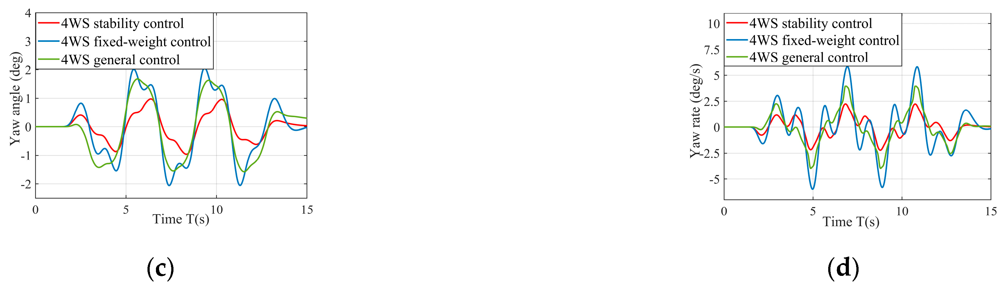
5.2. Serpentine Working Condition Simulation

To assess the handling stability of 4WS under a proposed hierarchical control strategy, a simulation of serpentine working conditions was performed, with a comparison made with two other strategies: (1) the “4WS general control”, where its upper motion controller implements the MPC method to control the sideslip angle, yaw rate, and longitudinal speed without considering the adjustment of the motion state reference value and weight coefficient, with the lower torque distribution only using the first level; (2) the “4WS fixed-weight control”, where its upper motion controller uses the MPC method, considering the adjustment to the coefficients but without considering the adaptive adjustment to the weight matrices for the vehicle stable-state coefficients.

For the serpentine experimental condition, the expected longitudinal speed was set to 65 km/h, and the adhesion coefficient was held constant at 0.8. The simulation results of the motion state, torque distribution, and stability parameters are presented in Figure 14, Figure 15, and Figure 16, respectively.

As depicted in Figure 14, the proposed hierarchical stability control strategy for 4WS enhances the trajectory tracking precision under serpentine working conditions when compared to the 4WS general control and 4WS fixed-weight control. Specifically, Figure 14a–d compare the trajectory, lateral deviation, speed, and front and rear wheel angles under the serpentine working condition of the three control strategies, respectively.

In Figure 14a,b, it can be observed that all three control methods can track the reference trajectory and that there is no lateral deviation when the vehicle is driving in the first straight section. When the vehicle initially drives around the pile, all three control strategies can better track the reference trajectory, and there is a certain lateral deviation. Here, the difference between the proposed 4WS stability control and the 4WS fixed-weight control is smaller. However, the partial enlarged detail indicates that the trajectory tracking performance of the proposed 4WS stability control strategy is superior, and the corresponding lateral deviation is always the smallest, around 50% lower than that of the 4WS fixed-weight control. Thus, the proposed 4WS stability control strategy achieves a higher trajectory tracking control accuracy. Meanwhile, the lateral deviation in the 4WS general control is the biggest, implying that adjusting the weight matrices based on the vehicle stability state coefficient can enhance the trajectory tracking accuracy of the 4WS vehicle. When the vehicle enters subsequent pile-winding driving, the difference in the lateral deviation among the three control strategies is similar to that of the pile-winding driving, and the 4WS control strategy can quickly return to straight driving after the end of the pile-winding driving. In conjunction with Figure 14d, it can also be observed that the front and rear wheel steering angle changes in the proposed 4WS stability control strategy are the smallest and the transition is the smoothest, with the peak steering angle being approximately 84% of that of the 4WS fixed-weight control. Consequently, the proposed 4WS stability control could realize the steering motion of the DDEVs with smaller front and rear wheel steering angles and quickly return to the straight driving state.

As shown in Figure 15, the proposed 4WS stability control strategy outperforms the 4WS fixed-weight control and 4WS general control in terms of the wheel motor torque output under serpentine working conditions. Figure 15a,d present the torque distribution results of the four motors under serpentine working conditions for these three control strategies. Specifically, the torque allocated to each wheel motor by the three control methods is similar when the vehicle is driving in a straight line, as indicated in Figure 15a,b. However, when the vehicle is driving around the pile, all three control methods can achieve an additional yaw moment by allocating different output torques to the four wheel motors while satisfying the peak torque limit. The proposed 4WS stability control strategy has the most uniform torque distribution and the smoothest control, as well as the smallest maximum motor output torque of approximately 30 Nm compared to 150 Nm for the 4WS fixed-weight control. This is due to the fact that the proposed strategy considers the vehicle’s handling stability when designing the control weight matrix, which leads to a smoother torque distribution control. Consequently, the proposed 4WS stability strategy can reduce the demand for wheel motor torque and complete serpentine winding with a smoother torque distribution.

In Figure 16, it is evident that the proposed 4WS stability control enhances the handling stability of the vehicle under the serpentine working condition, in comparison to the 4WS fixed-weight control and 4WS general control. Figure 16a–d depict the variations in the tire sideslip angle, total tire load rate, yaw angle error, and yaw rate, respectively, for these three control strategies under the serpentine working condition. It can be observed in Figure 16a,b that all three control methods maintain stability when the vehicle navigates around the pile in a high-speed snake. The stability margin difference between the proposed 4WS stability control and the 4WS fixed-weight control is negligible, but the proposed 4WS stability control strategy exhibits the much larger stability margin than the 4WS general control. By optimizing the torque distribution with the minimum tire load rate as the objective function, the total tire load rate of the proposed 4WS stability control is reduced by approximately 35% compared to that of the 4WS general control. Additionally, the tire sideslip angle is significantly decreased, which indicates improved handling stability of the vehicle. Figure 16c,d illustrate that the proposed 4WS stability control significantly reduces the yaw angle deviation and yaw rate in comparison to the 4WS fixed-weight control and 4WS general control, reducing them by approximately 50% and 66%, respectively. This reduction enables the vehicle to achieve the desired yaw tracking motion. The findings demonstrate that the proposed 4WS stability control strategy can accomplish steady-state steering by ensuring the desired vehicle motion.

6. Conclusions

This paper presented a hierarchical control strategy for the handling stability of DDEVs with 4WS based on a phase plane analysis. Firstly, a dynamic model for the 4WS of DDEVs was established, and a reference motion state equation for the handling stability control was derived. Secondly, a phase plane analysis was utilized to compare the stable area of the phase plane and to analyze the impacts of the front and rear wheel angles, longitudinal speed, and road adhesion coefficient on vehicle stability. A hierarchical control strategy was proposed, consisting of an upper motion control based on an MPC and a lower torque distribution control based on a two-level optimal distribution algorithm. The front and rear wheel angles and additional yaw moment were chosen as the control variables, while the yaw rate and the sideslip angle of the center of mass were chosen as the state variables. Moreover, the optimal distribution of the output torque for the four wheel motors was obtained through a two-level optimal distribution algorithm. Finally, the proposed control strategy was evaluated via co-simulation using the CarSim and MATLAB/Simulink software. The results of the double lane change condition and serpentine working condition experiments demonstrate that the presented control strategy could significantly enhance the handling stability of DDEVs with 4WS, reducing the total tire load rate by 66.6% and 35.3% compared to the general control of 4WS.

References

1. Fu, W.; Liu, Y.; Zhang, X. Research on Accurate Motion Trajectory Control Method of Four-Wheel Steering AGV Based on Stanley-PID Control. Sensors 2023, 23, 7219. [Google Scholar] [CrossRef]
2. Lai, F.; Huang, C. Path tracking and stability integrated control of intelligent vehicles under steering collision avoidance. Proc. Inst. Mech. Eng. Part D J. Automob. Eng. 2023, 237, 1868–1884. [Google Scholar] [CrossRef]
3. Su, L.; Wang, Z.; Chen, C. Torque vectoring control system for distributed drive electric bus under complicated driving conditions. Assem. Autom. 2022, 42, 1–18. [Google Scholar] [CrossRef]
4. Liang, Z.; Shen, M.; Zhao, J.; Li, Z.; Ding, Z. Adaptive Sliding Mode Fault Tolerant Control for Autonomous Vehicle with Unknown Actuator Parameters and Saturated Tire Force Based on the Center of Percussion. IEEE Trans. Int. Transp. Syst. 2023, 24, 11595–11606. [Google Scholar] [CrossRef]
5. Lei, Y.; Wen, G.; Fu, Y.; Li, X.; Hou, B.; Geng, X. Trajectory-following of a 4WID-4WIS vehicle via feedforward–backstepping sliding-mode control. Proc. Inst. Mech. Eng. Part D J. Automob. Eng. 2022, 236, 322–333. [Google Scholar] [CrossRef]
6. Lu, M.; Xu, Z. Integrated Handling and Stability Control with AFS and DYC for 4WID–EVs via Dual Sliding Mode Control. Autom. Control Comp. Sci. 2021, 55, 243–252. [Google Scholar]
7. Silva, F.; Silva, L.; Eckert, J.; Yamashita, R.; Lourenco, M. Parameter influence analysis in an optimized fuzzy stability control for a four-wheel independent-drive electric vehicle. Control Eng. Pract. 2021, 120, 105000. [Google Scholar] [CrossRef]
8. Zhang, D.; Song, Q.; Wang, G.; Liu, C. A Novel Longitudinal Speed Estimator for Four-Wheel Slip in Snowy Conditions. Appl. Sci. 2021, 11, 2809. [Google Scholar] [CrossRef]
9. Zheng, H.; Yang, S.; Li, B. Optimization Control for 4WIS Electric Vehicle Based on the Coincidence Degree of Wheel Steering Centers. SAE Int. J. Veh. Dyn. Stab. NVH 2018, 2, 169–184. [Google Scholar] [CrossRef]
10. Xu, T.; Zhao, Y.; Wang, Q.; Deng, H.; Lin, F. An Adaptive Inverse Model Control Method of Vehicle Yaw Stability with Active Front Steering Based on Adaptive RBF Neural Networks. IEEE Trans. Veh. Technol. 2023, 72, 13873–13887. [Google Scholar] [CrossRef]
11. Botes, W.; Botha, T.; Els, P. Real-time lateral stability and steering characteristic control using non-linear model predictive control. Veh. Syst. Dyn. 2023, 61, 1063–1085. [Google Scholar] [CrossRef]
12. Tan, Q.; Qiu, C.; Huang, J.; Yin, Y.; Zhang, X.; Liu, H. Path tracking control strategy for off-road 4WS4WD vehicle based on robust model predictive control. Rob. Autonom. Syst. 2022, 158, 104267. [Google Scholar] [CrossRef]
13. Zhang, N.; Wang, J.; Li, Z.; Xu, N.; Ding, H.; Zhang, Z.; Guo, K.; Xu, H. Coordinated Optimal Control of AFS and DYC for Four-Wheel Independent Drive Electric Vehicles Based on MAS Model. Sensors 2023, 23, 3505. [Google Scholar] [CrossRef] [PubMed]
14. Hang, P.; Chen, X. Integrated chassis control algorithm design for path tracking based on four-wheel steering and direct yaw-moment control. Proc. Inst. Mech. Eng. Part I J. Syst. Control Eng. 2019, 233, 625–641. [Google Scholar] [CrossRef]
15. Wang, C.; Heng, B.; Zhao, W. Yaw and lateral stability control for four-wheel-independent steering and four-wheel-independent driving electric vehicle. Proc. Inst. Mech. Eng. Part D J. Automob. Eng. 2020, 234, 409–422. [Google Scholar] [CrossRef]
16. Hang, P.; Xia, X.; Chen, X. Handling Stability Advancement With 4WS and DYC Coordinated Control: A Gain-Scheduled Robust Control Approach. IEEE Trans. Veh. Technol. 2021, 70, 3164–3174. [Google Scholar] [CrossRef]
17. Taghavifar, H.; Hu, C.; Taghavifar, L.; Qin, Y.; Na, J.; Wei, C. Optimal robust control of vehicle lateral stability using damped least-square backpropagation training of neural networks. Neurocomputing 2020, 384, 256–267. [Google Scholar] [CrossRef]
18. Tian, J.; Ding, J.; Zhang, C.; Luo, S. Four-Wheel Differential Steering Control of IWM Driven EVs. IEEE Access 2020, 8, 152963–152974. [Google Scholar] [CrossRef]
19. Ge, L.; Shan, Z.; Ma, F.; Han, Z.; Guo, K. Simultaneous Stability and Path Following Control for 4WIS4WID Autonomous Vehicles Based on Computationally Efficient Offset Free MPC. Int. J. Control Autom. Syst. 2023, 21, 2782–2796. [Google Scholar] [CrossRef]
20. Shi, K.; Yuan, X.; He, Q. Double-layer Dynamic Decoupling Control System for the Yaw Stability of Four Wheel Steering Vehicle. Int. J. Control Autom. Syst. 2019, 17, 1255–1263. [Google Scholar] [CrossRef]
21. Marino, R.; Cinili, F. Input-output decoupling control by measurement feedback in four-wheel-steering vehicles. IEEE Trans. Control Syst. Technol. 2019, 17, 1163–1172. [Google Scholar] [CrossRef]
22. Park, J.Y.; Na, S.; Cha, H.; Yi, K. Direct Yaw Moment Control with 4WD Torque-Vectoring for Vehicle Handling Stability and Agility. Int. J. Automot. Technol. 2022, 23, 555–565. [Google Scholar] [CrossRef]
23. Wu, H.; Li, Y. Coordination Control of Path Tracking and Stability for 4WS Autonomous Vehicle. In Proceedings of the 2020 International Conference on Electromechanical Control Technology and Transportation (ICECTT), Nanchang, China, 15–17 May 2020; pp. 343–348. [Google Scholar]
24. Wang, Q.; Zhao, Y.; Deng, Y.; Xu, H.; Deng, H.; Lin, F. Optimal Coordinated Control of ARS and DYC for Four-Wheel Steer and In-Wheel Motor Driven Electric Vehicle With Unknown Tire Model. IEEE Trans. Veh. Technol. 2020, 69, 10809–10819. [Google Scholar] [CrossRef]
25. Sakhnevych, A.; Arricale, V.M.; Bruschetta, M.; Censi, A.; Mion, E.; Picotti, E.; Frazzoli, E. Investigation on the Model-Based Control Performance in Vehicle Safety Critical Scenarios with Varying Tyre Limits. Sensors 2021, 21, 5372. [Google Scholar] [CrossRef] [PubMed]
26. Song, Y.; Shu, H.; Chen, X.; Luo, S. Direct-yaw-moment control of four-wheel-drive electrical vehicle based on lateral tyre–road forces and sideslip angle observer. IET Int. Trans. Syst. 2019, 13, 303–312. [Google Scholar] [CrossRef]
27. Yakub, F.; Mori, Y. Comparative study of autonomous path-following vehicle control via model predictive control and linear quadratic control. Proc. Inst. Mech. Eng. Part D J. Automob. Eng. 2015, 229, 1695–1714. [Google Scholar] [CrossRef]
28. Dong, Q.; Ji, X.; Liu, Y.; Liu, Y. Gain-Scheduled Steering and Braking Coordinated Control in Path Tracking of Intelligent Heavy Vehicles. ASME. J. Dyn. Sys. Meas. Control 2022, 144, 101006. [Google Scholar] [CrossRef]
29. Yakub, F.; Muhammad, P.; Toh, H.T.; Talip, M.; Mori, Y. Explicit controller of a single truck stability and rollover mitigation. J. Mech. Sci. Technol. 2018, 32, 4373–4381. [Google Scholar] [CrossRef]
30. Zhai, L.; Wang, C.; Hou, Y.; Hou, R.; Yuh, M.; Zhang, X. Two-level optimal torque distribution for handling stability control of a four hub-motor independent-drive electric vehicle under various adhesion conditions. Proc. Inst. Mech. Eng. Part D J. Automob. Eng. 2022, 237, 544–559. [Google Scholar] [CrossRef]
Figure 1. Nonlinear 7 DOF model of four-wheel steering.
Machines 12 00478 g001
Figure 2. Wheel rotation model.
Machines 12 00478 g002
Figure 3. Linear 2-DOF model of four-wheel steering.
Machines 12 00478 g003
Figure 4. Influence of the steering angles of the front and rear wheels on the stable region ( v x = 60   km / h and μ = 0.8 ): (a) δ f = 3 deg ,   δ r = 0 ; (b) δ f = 6 deg ,   δ r = 0 ; (c) δ f = 0 ,   δ r = 3 deg ; (d) δ f = 0 ,   δ r = 6 deg ; (e) δ f = 3 deg ,   δ r = 3 deg ; (f) δ f = 6 deg ,   δ r = 6 deg ; (g) δ f = 3 deg ,   δ r = 3 deg ; and (h) δ f = 6 deg ,   δ r = 6 deg .
Machines 12 00478 g004aMachines 12 00478 g004b
Figure 5. Influence of the road adhesion coefficient on the stable region ( v x = 80 km / h and δ f = 0 , δ r = 0 ): (a) μ = 0.2 ; (b) μ = 0.4 ; (c) μ = 0.6 ; and (d) μ = 0.8 .
Machines 12 00478 g005aMachines 12 00478 g005b
Figure 6. Influence of the longitudinal vehicle speed on the stable region ( μ = 0.8 and δ f = 0 , δ r = 0 ): (a) v x = 20 km / h ; (b) v x = 50 km / h ; (c) v x = 80 km / h ; and (d) v x = 110 km / h .
Machines 12 00478 g006
Figure 7. Boundary coefficients under different steering angles of the front and rear wheels.
Machines 12 00478 g007
Figure 8. Framework of hierarchical control strategy for handling stability.
Machines 12 00478 g008
Figure 9. Framework of MPC motion controller.
Machines 12 00478 g009
Figure 10. The relationship between weight matrices Q β and Q γ .
Machines 12 00478 g010
Figure 11. Simulation results of motion state under double lane change conditions: (a) trajectory; (b) lateral deviation; (c) longitudinal speed; and (d) front and rear wheel angles (the solid line represents the front wheel and the dotted line represents the rear wheel).
Machines 12 00478 g011
Figure 12. Simulation results of torque distribution under double lane change conditions: (a) torque of left front wheel; (b) torque of right front wheel; (c) torque of left rear wheel; and (d) torque of right rear wheel.
Machines 12 00478 g012
Figure 13. Simulation results of stability parameters under double lane change conditions: (a) sideslip angle; (b) total of tire load rate; (c) yaw angle; and (d) yaw rate.
Machines 12 00478 g013aMachines 12 00478 g013b
Figure 14. Simulation results of motion state under serpentine working conditions: (a) trajectory; (b) lateral deviation; (c) longitudinal speed; and (d) front and rear wheel angles (the solid line represents the front wheel and the dotted line represents the rear wheel).
Machines 12 00478 g014
Figure 15. Simulation results of torque distribution under serpentine working conditions: (a) torque of left front wheel; (b) torque of right front wheel; (c) torque of left rear wheel; and (d) torque of right rear wheel.
Machines 12 00478 g015
Figure 16. Simulation results of stability parameters under serpentine working conditions: (a) sideslip angle; (b) total of tire load rate; (c) yaw angle error; and (d) yaw rate.
Machines 12 00478 g016aMachines 12 00478 g016b