Determination of Energy Losses of the Crank Press Mechanism

Abstract

This paper focuses on determining the friction energy loss in the mechanism of a mechanical crank press. After defining the crank press mechanism and how it works, we describe the energy balance of a technological operation—forming. Four distinct methodologies for calculating friction loss in the mechanism are then presented, namely an empirical method, a spreadsheet calculation utilising force decomposition in a crank mechanism, an analytical calculation of the dynamic behaviour of a press, and a multibody simulation. Each additional approach expands the possibilities for approaching reality, but as the primary aim of the study is to compare the approaches, these possibilities are not exploited. Multibody simulation has proved itself to be accurate and suitable for simulating press mechanisms and investigating their dynamics. Multibody simulation is a much more powerful tool that can lead to a digital twin, which can help us to develop a less energy-demanding press. Confirmation of the multibody simulation results is the main outcome of the comparison and will be used in future work.

1. Introduction

The crank mechanism is used in forging presses, which are widely used in (but not limited to) the automotive industry. Due to the high impact forces involved in forging, plain bearings are used in the crank mechanism of a forging press because of their high load-carrying capacity. A typical bearing in such a machine consists of a steel shaft and a bronze bushing mounted between two steel housing halves. Plain bearings in the press mechanism are a source of relatively high friction losses [1]. Plain bearings in forging presses are lubricated with grease or oil. Grease lubrication is typically used to mitigate potential damage to the lubricating film under high impact loads, despite its higher frictional losses compared to oil lubrication [2]. Oil-lubricated plain bearings are commonly used in high-speed rotating machinery, but mechanical presses tend to operate at low speeds.

Our general goal is to explain the formation of friction losses during the forging phase of a press stroke, optimize the press design, and reduce energy costs [3]. Our secondary aim is to compare four different methods to identify their advantages, suitability, and difficulty of use in the design phase of a new machine.

Methods compared include the following:

• Empirical Method (Section 4)
• Calculation in a Spreadsheet (Section 5)
• Analytical Calculation (Section 6)
• Multibody Simulation (Section 7)

There are traditional approaches to counting energy losses. The most straightforward approach was developed by our predecessors through observation and measurement of real machines—empirical relationships. Other approaches have been based on simple kinematic description and static force analysis of the crank mechanism [4]. Modern approaches are based on computer simulations of the kinematics. Within these simulations, the dynamics or flexibility of the mechanism can be considered. This article focuses on the verification of multibody simulations for future use.

In this article, we only focus on the machine side of the press, without considering the drive side, which also has an important influence on energy efficiency.

2. Description of Crank Press Mechanism

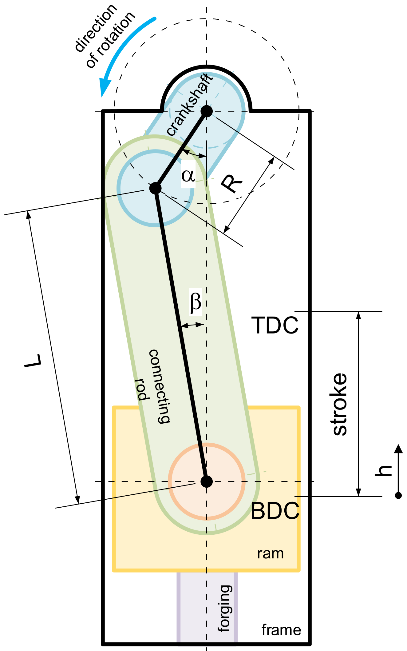
The crank press mechanism consists of a crankshaft, connecting rod, and ram, as shown in Figure 1. In our setup, the connecting rod is connected to the ram by a pin passing through the ram. The mechanism is mounted in a robust frame that is under a working load.

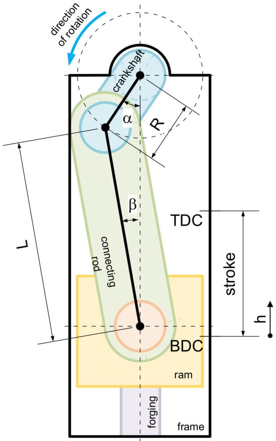
Figure 1. Diagram of the crank press mechanism.

The press drive is connected to the mechanism via the crankshaft. The drive typically consists of an electric motor powering a flywheel, which is usually mounted on a countershaft. The energy accumulated in the flywheel is transferred to the crankshaft through a friction clutch. To stop and secure the mechanism at top dead centre (TDC), a brake is installed. As this article does not address energy losses in the drive part of the crank press, it does not consider these losses.

2.1. Kinematic Relations

To perform an energy analysis of the friction losses in the machine mechanism, it is necessary to know the dependence of the ram position h on the rotation of the crankshaft α. For the mechanism shown in Figure 1, the formula is as follows:

$$h=R·\left(1-\cos \alpha +\frac{R}{L}·\frac{{sin}^2\alpha }{2}\right)$$

(1)

where $h$ is ram position (from BDC)—current stroke; $R$ is crank radius—eccentricity of crankshaft; $L$ is connecting rod length; and $\alpha$ is the crank angle (from BDC).

2.2. Static Force Analysis

Understanding the forces acting in the mechanism is crucial to determining friction losses. The following figure shows the force decomposition in the crank mechanism. This is not affected by frictional forces. However, there are also friction torques in separate contact pairs. These are shown in the same Figure 2 [5,6].

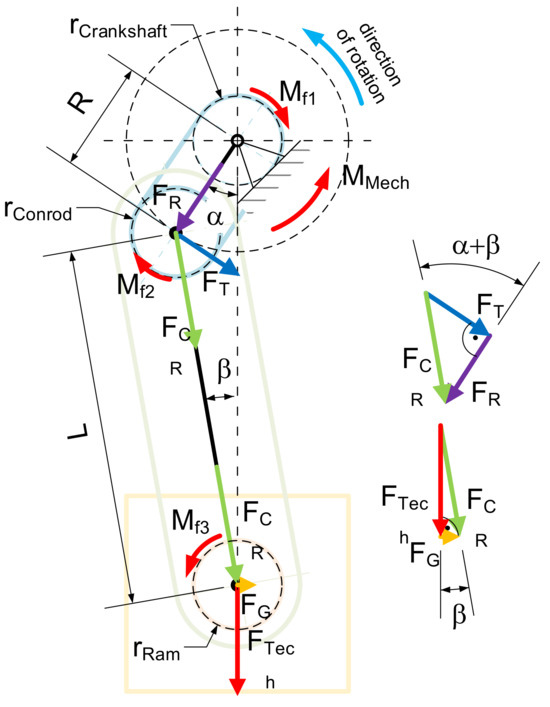
Figure 2. Force decomposition of a crank mechanism.

The following formulae are for the forces and torques in the crank mechanism (Figure 2).

Force in the connecting rod $F_{CR}$ is as follows:

$$F_{CR}=\frac{F_{Tech}}{\cos \left(\beta \right)}$$

(2)

where $F_{CR}$ is the internal force in the connecting rod [N]; $F_{Tech}$ is the technology force (forged material resistance) [N]; and $\beta$ is the angle between the connecting rod and mechanism axis [rad].

Force acting on the linear guide $F_G$ is as follows:

$$F_G=\frac{F_{Tech}}{\sin \left(\beta \right)}$$

(3)

In this paper, the influence of the force acting on the linear guide $F_G$ is neglected. This force causes a friction loss between the ram and its linear guide. The magnitude of this loss is much smaller than the other types of friction losses.

At this point, the force in the connecting rod, $F_{CR}$, is divided into the tangential force, $F_T$, and the radial force, $F_R$.

$$\begin{array}{l}{F}_T=F_{CR}·\cos \alpha \\ F_R=F_{CR}·\sin \alpha \end{array}$$

(4)

To induce the technological force $F_{Tech}$, it is necessary to apply the following torque $M_{Mech}$ to the crankshaft.

$$M_{Mech}=F_T·R=F_{CR}·\cos \alpha ·R=F_{Tech}·R·\frac{\cos \alpha }{\cos \beta }$$

(5)

The following frictional torques, acting against the direction of movement, are induced in the connections of the parts of the crank mechanism. Torque $M_{f1}$ is a frictional torque induced between the crankshaft and its bearings in the machine frame.

$$M_{f1}=F_{CR}·\mu ·\frac{d_{Crankshaft}}{2}$$

(6)

where $\mu$ is coefficient of friction [1]; and $d_{Crankshaft}$ is diameter of the crankshaft journal in the stand [m].

Torque $M_{f2}$ is a frictional torque induced between the crankshaft and its bearing in the connecting rod.

$$M_{f2}=F_{CR}·\mu ·\frac{d_{Conrod}}{2}$$

(7)

where $d_{Conrod}$ is diameter of the crankshaft in the connecting rod [m].

Torque $M_{f3}$ is a frictional torque induced between the ram pin and the bearing in the connecting rod.

$$M_{f3}=F_{CR}·\mu ·\frac{d_{Ram}}{2}$$

(8)

where $d_{Ram}$ is diameter of the ram pin in the connecting rod [m].

To determine the drive torque $M_{Drive}$, the torque $M_{f3}$ is converted to the crankshaft. Here it acts as a torque ${M_{f3}}^{*}$.

$${M_{f3}}^{*}=\frac{R·\cos \alpha }{L·\cos \beta }·M_{f3}$$

(9)

where $R$ is crankshaft eccentricity [m]; and $L$ is length of connecting rod [m].

The drive torque is given as the sum of its component torques.

$$M_{Drive}=M_{Mech}+M_{f1}+M_{f2}+{M_{f3}}^{*}$$

(10)

Coefficient of Friction

The coefficient of friction has a significant effect on the friction losses, i.e., the amount of energy lost. Many analyses have shown that the coefficient of friction is not constant. It is known that the coefficient of friction depends on the relative speed of bodies in contact [7]. In the case of lubricated contact, the friction losses depend on the viscosity of the lubricant, which usually depends on the temperature of the lubricant [8]. After reaching operating temperature, friction losses can be reduced by an order of magnitude compared to the cold state.

Although the coefficient of friction can be considered as a dependent function for simulation purposes [9], it was considered constant $\mu =0.03$ in our comparison.

2.3. An Analysis of Energy Flow in a Crank Press—Energy Balance

The energy balance equation (the amount of energy that a drive must deliver to a mechanism (machine) to perform its technical operation) is solved for one work cycle during the continuous operation of the machine [10].

$$A_c=A_u\pm A_d+A_f\pm A_a\pm A_g$$

(11)

where $A_c$ is Total work; $A_u$ is Useful work; $A_d$ is Work of elastic deformations; $A_f$ is Friction work (loss); $A_a$ is Work of acceleration of masses; and $A_g$ is Work of gravity.

The energy balance of a forming machine can also be evaluated for a discontinuous work cycle. A discontinuous work cycle is one in which, after each technological operation, the crank shaft and the connected ram stop in the upper dead centre of the mechanism. This means that the energy is calculated from the time the drive and the crank shaft of the mechanism are connected by the clutch to the time they are disconnected from the clutch, and the crankshaft is stopped by the brake. The energy required to start the machine is not included in the energy balance formula.

3. Parameters of a Real Forging Press

The following Table 1 shows the parameters of a real forging press.

Table 1. Parameters of a real press.

$F_{Nom}$	$25 \mathrm{M}\mathrm{N}$	Nominal forming force
$R$	$160 \mathrm{m}\mathrm{m}$	Crankshaft eccentricity
$L$	$1 075 \mathrm{m}\mathrm{m}$	Length of connecting rod
$d_{Crankshaft}$	$540 \mathrm{m}\mathrm{m}$	Diameter of the crankshaft in the stand
$d_{Conrod}$	$870 \mathrm{m}\mathrm{m}$	Diameter of the crankshaft in the conrod
$d_{Ram}$	$620 \mathrm{m}\mathrm{m}$	Diameter of the ram shaft in the conrod
$\mu$	$0.03$	Coefficient of friction
$n$	$70/\mathrm{m}\mathrm{i}\mathrm{n}$	Number of strokes per minute

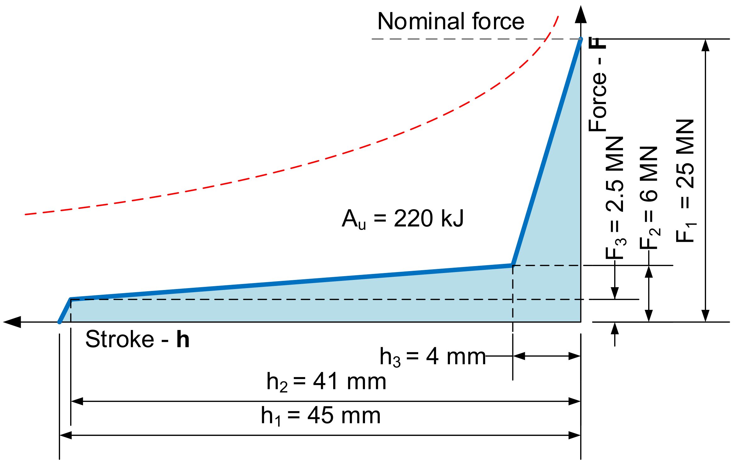
As the example is made for a crank forging press, a simplified die-forming characteristic is considered for the subsequent load simulation. The considered shape of the technological force curve is shown in the following Figure 3. The expected useful work of this technology is 220 kJ.

Figure 3. A force–displacement curve representing closed die forging for a 25 MN crank press.

The technological force $F_{Tech}$ is equal to the nominal force $F_{Nom}$ of the press for further calculations.

4. Empirical Method for Enumerating Friction Losses

The historical method of designing a mechanical forging press is based on the experience gained during decades of production of these machines (SMERAL, Brno, Czech Republic, former Czechoslovakia). All partial work is calculated as part of the useful work, except for the work consumed by elastic deformation of the machine and tools.

Work of Friction (Loss)

According to [11], the friction work equals 0.8 ÷ 1 of the useful work. However, these sources only provide figures for machines with flexible stands (Table 2).

$$A_{fy}=\left(0.8÷1\right)·A_u=\left(0.8÷1\right)·220=176÷220 \mathrm{k}\mathrm{J}$$

(12)

Table 2. Results of empirical method.

	AMech	Af1	Af2	Af3	Az	ADrive
	kJ
Empiric	220	n/a	n/a	n/a	(176 ÷ 220) For a press with a flexible stand!	396 ÷ 440

5. Determination by Calculation in a Spreadsheet

Please keep the following text in mind:

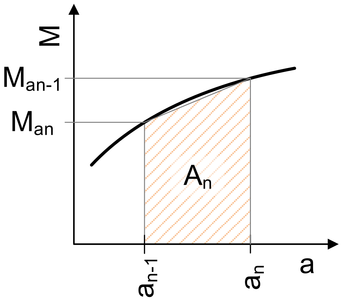
The calculation of partial moments and the work derived from them was carried out in a spreadsheet program (e.g., MS Excel 2013). The calculations were based on force decomposition as described in the Static Force Analysis chapter. The primary goal was to determine the friction loss work. The angle of rotation was divided into small increments (e.g., 0.5°) in the table. The work was determined by numerical integration (using the trapezoidal rule [12]) of the friction torque curve (refer to Figure 4).

Figure 4. An example of numerical integration (trapezoidal rule) of a torque versus crankshaft angle plot.

The integration formula is as follows:

$$A_{Mech}=\frac{{\alpha }_n-{\alpha }_{n-1}}{2}·\frac{M_{Mech n-1}+M_{Mech n}}{2}$$

(13)

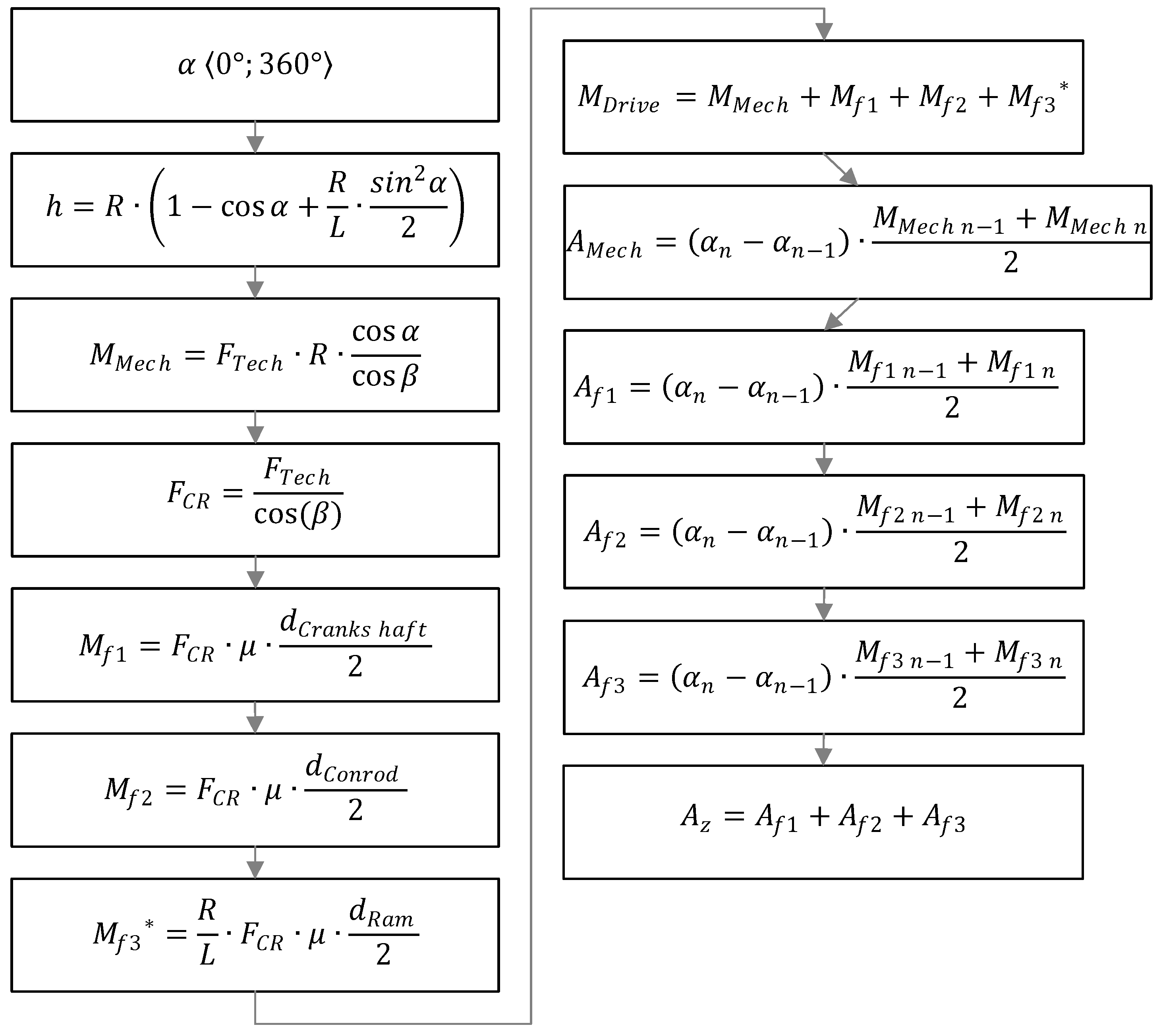
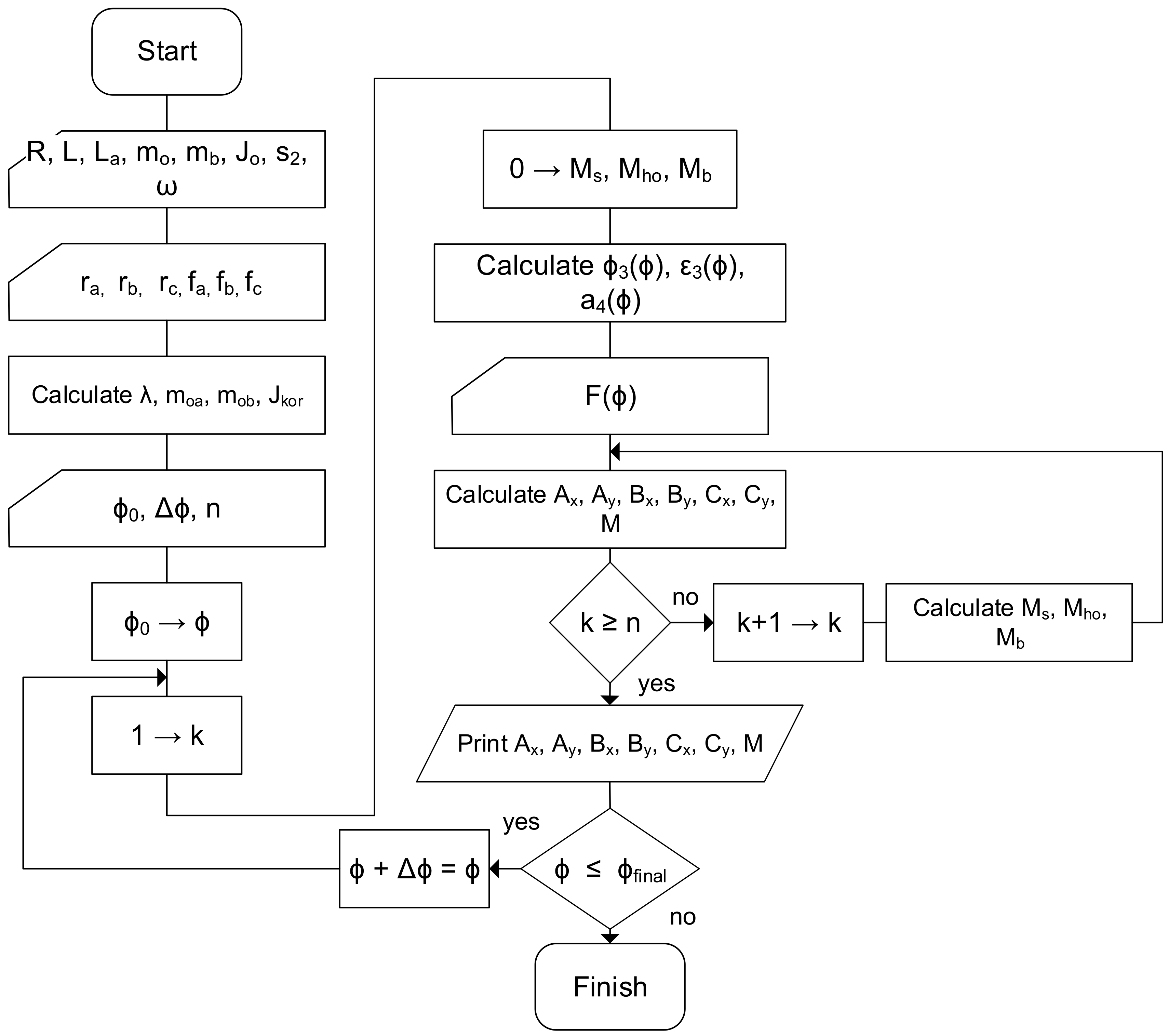
The following flow chart (Figure 5) illustrates the calculation using the spreadsheet.

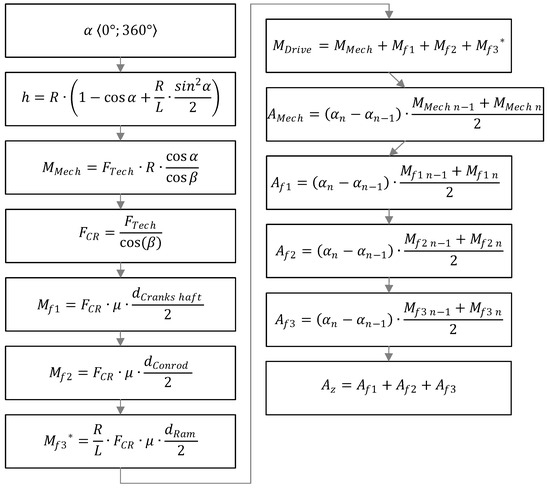
Figure 5. Spreadsheet calculation flowchart.

5.1. Initial Conditions

It is the initial conditions of the calculation that make the difference between the different approaches (which this study aims to compare). As the complexity of the calculation increases, so does the ability to account for initial conditions and thus its realistic accuracy. We considered the following initial conditions in this paper:

• Rigid body mechanism—determines whether the bodies of the mechanism (press structure) are absolutely rigid or flexible. This criterion affects not only the energy consumed by elastic deformations.
• Angular velocity of the crankshaft—determines whether the considered angular velocity of the crankshaft is constant or depends (state is dependent) on the kinetic energy of the system.
• Inertial forces—is the criterion determining whether inertial forces are included in the calculation. States are neglected or included.
• Gravitational acceleration—is the criterion determining whether gravitational acceleration is included in the calculation. States are neglected or included.
• Weight balancing—is the criterion determining whether the weight balancing (the device of the mechanical press overloading its ram and crank mechanism due to the definition of clearances in the bearings) is included in the calculation. States are neglected or included.

The initial conditions of the Calculation in a Spreadsheet are as follows (Table 3):

Table 3. The initial conditions of Calculation in a Spreadsheet.

	Status
Rigid body mechanism	rigid
Angular velocity of the crankshaft	constant
Inertial forces	neglected
Gravitational acceleration	neglected
Weight balancing	neglected

5.2. Results of Calculation in a Spreadsheet

Figure 6 shows the results of the torques within the crank mechanism from a spreadsheet calculation. It can be seen that the value of the torque $M_{mech}$ decreases to zero upon reaching BDC, which is due to the mechanical advantage also reaching zero [11]. However, the friction torque values increase due to the increasing load of the technological force.

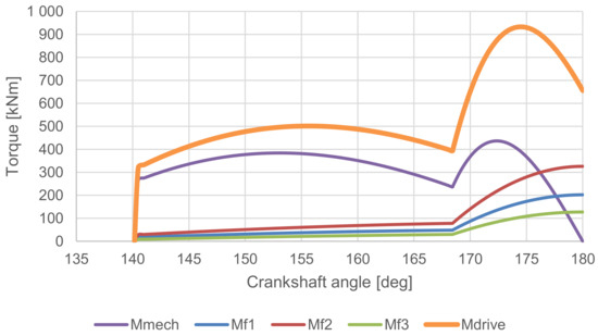
Figure 6. The graph of torques versus crankshaft angle—Calculation in a Spreadsheet.

The friction work values in Table 4 are as expected. For example, the friction work $A_{\mathrm{f}1}$ is comparatively smaller than $A_{\mathrm{f}2}$ because the friction radius ${\mathrm{r}}_{\mathrm{C}\mathrm{r}\mathrm{a}\mathrm{n}\mathrm{k}\mathrm{s}\mathrm{h}\mathrm{a}\mathrm{f}\mathrm{t}}$ is smaller than the friction radius ${\mathrm{r}}_{\mathrm{C}\mathrm{o}\mathrm{n}\mathrm{r}\mathrm{o}\mathrm{d}}$ by the same ratio. Similarly, the friction work $A_{\mathrm{f}3}$ is smaller than the others due to the smaller pin radius ${\mathrm{r}}_{\mathrm{R}\mathrm{a}\mathrm{m}}$ and, at the same time, the swing angle of the connecting rod is smaller than the swing angle of the crankshaft.

Table 4. Results of Calculation in a Spreadsheet.

	AMech	Af1	Af2	Af3	Az	ADrive
	kJ
Calculation in a Spreadsheet	224	50	82	9	141	364

6. Analytical Calculation of the Dynamic Behaviour of the Mechanism

The interaction of the body with external forces and moments can be studied by breaking down a work cycle into multiple steps. If the force and moment are both zero, the external forces form a zero-equivalent system, and the rigid body is in equilibrium according to the following conditions [13]:

$$\sum \mathit{F}=0, \sum \mathit{M}=\sum (\mathit{r}\times \mathit{F})=\mathbf{0}$$

(14)

This method is highly versatile and is suitable for mechanisms with an unlimited number of degrees of freedom. It also allows for the inclusion of frictional resistances against movement. This method enables the calculation of reaction forces in the joints.

The method of solving dynamic problems involves the creation of free-body diagrams and the identification of all external forces and moments. Once all the acting forces have been identified, a system of equations can be set up with joint reactions as unknown variables. In order to facilitate the solution of each individual step of the calculation, it is necessary to set up the equations with the crankshaft angle α as a variable.

From a mathematical perspective, we have obtained a system of algebraic–differential equations. The addition of passive effects renders the system nonlinear, which can be readily solved using the “fsolve solver” function. A multitude of software programs are equipped with this functionality, with MATLAB R2023 being a case in point.

The initial conditions of Analytical Dynamic Calculation are as follows (Table 5):

Table 5. The initial conditions of Analytical Dynamic Calculation.

	Status
Rigid body mechanism	rigid
Angular velocity of the crankshaft	constant
Inertial forces	included
Gravitational acceleration	included
Weight balancing	neglected

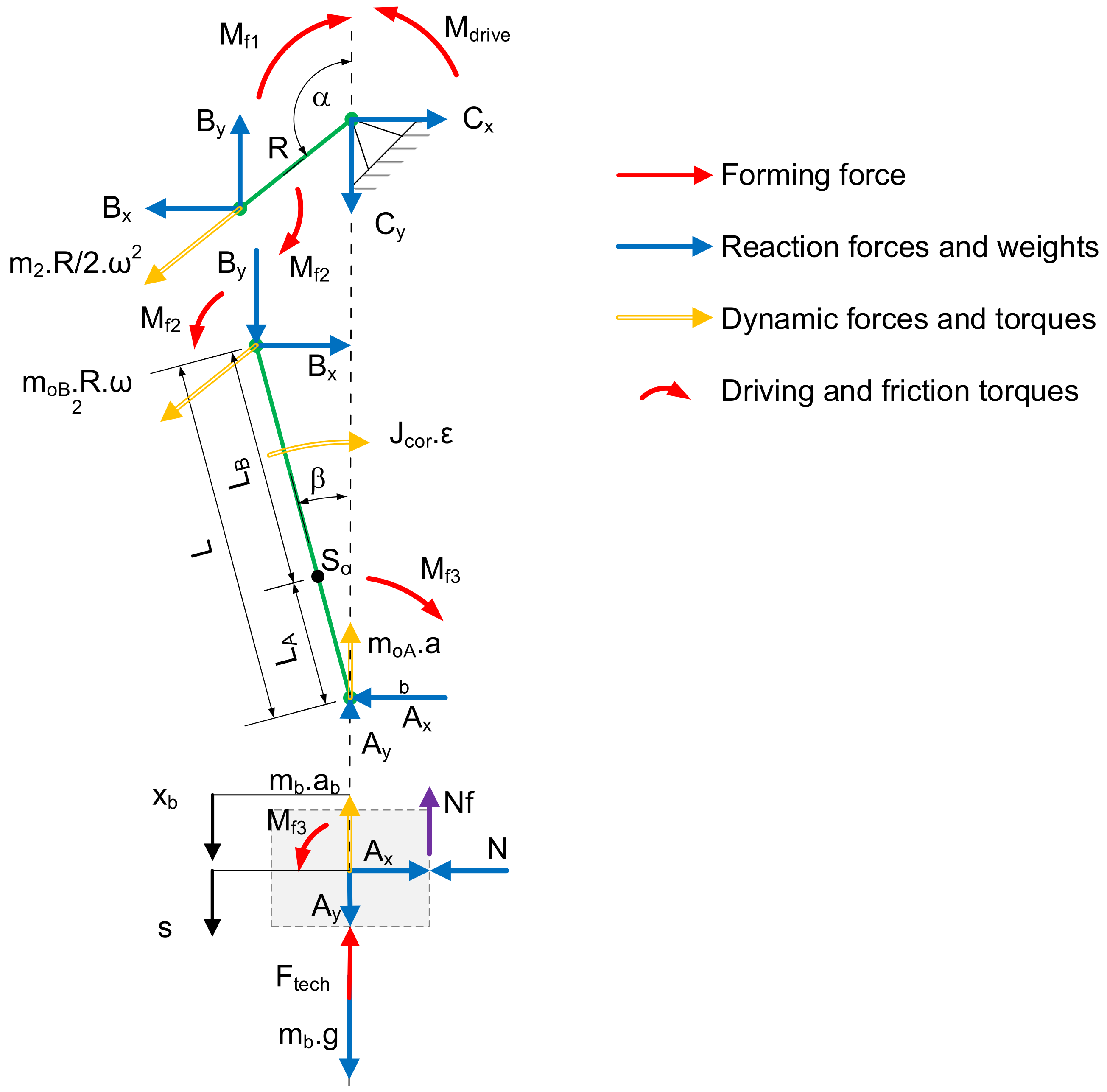
The decomposition of force and torque in a press mechanism is as follows (Figure 7):

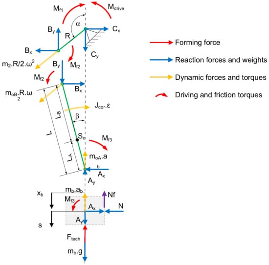
Figure 7. Free-body diagrams—force and torque decomposition of a press mechanism.

The system of nonlinear equations that describes the crank mechanism, along with the algorithm for solving a system of nonlinear equations, are presented in Figure 8.

$$\begin{array}{l}F\left(1\right)=A_x-N=x\left(2\right)-x\left(1\right)\\ F\left(2\right)=F_o-m_{b}g+m_b{a}_b+fN-A_y=F_{tech}-m_{b}g+m_b{a}_b+fx\left(1\right)-x\left(3\right)\\ F\left(3\right)=A_{x}L·\mathrm{c}\mathrm{o}\mathrm{s}\beta -\left(A_y+m_{oA}{a}_b\right)L·sin\beta +J_{kor}\epsilon +M_{f3}-M_{f2}=x\left(2\right)L·\mathrm{c}\mathrm{o}\mathrm{s}\beta -\left(x\left(3\right)+m_{oA}{a}_b\right)L·sin\beta +J_{cor}\epsilon +M_{f3}-M_{f2}\\ F\left(4\right)=A_x+m_{oB}R{\omega }^2·sin\alpha -B_x=x\left(2\right)+m_{oB}R{\omega }^2·sin\alpha -x\left(4\right)\\ F\left(5\right)=A_y+m_{oA}{a}_b+m_{oB}R{\omega }^2·cos\alpha -B_y=x\left(3\right)+m_{oA}{a}_b+m_{oB}R{\omega }^2·cos\alpha -x\left(5\right)\\ F\left(6\right)=-B_{x}R·cos\alpha +B_{y}R·sin\alpha +M_{f1}-M_{f2}-M_{drive}=-x\left(4\right)R·cos\alpha +x\left(5\right)R·sin\alpha +M_s-M_{ho}-x\left(8\right)\\ F\left(7\right)=B_x+\frac{1}{2}{m}_{2}R{\omega }^2·sin\alpha -C_x=x\left(4\right)+\frac{1}{2}{m}_{2}R{\omega }^2·sin\alpha -x\left(6\right)\\ F\left(8\right)=B_y+\frac{1}{2}{m}_{2}R{\omega }^2·cos\alpha -C_y=x\left(5\right)+\frac{1}{2}{m}_{2}R{\omega }^2·cos\alpha -x\left(7\right)\end{array}$$

(15)

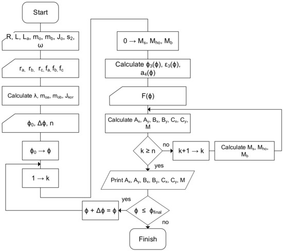
Figure 8. Flowchart of a analytical calculation.

After determining all the equations describing the equilibrium of the mechanism and its parts, we assembled a system from these equations. The solver of nonlinear systems of equations solved the following problem of the system (matrix) of equations $F$ depending on the vector of unknown $x$ [14].

$$\mathit{F}\left(\mathit{x}\right)=0$$

(16)

Accordingly, each row of the system of equations presented in Table 6 must be expressed as equal to zero. This signifies that all input and output quantities are on the same side. The command that performs the system solution is as follows:

x = fsolve(@(x)equations(x, alpha(1,i), Ftech(1,i)), x0);

(17)

Table 6. The results of the Analytical Dynamic Calculation.

	AMech	Af1	Af2	Af3	Az	ADrive
	kJ
Analytical Dynamic Calculation	224	50	81	9	140	376

This command says that the vector x is the output of the fsolve solver, which processes the equations from the set called “equations” for the crankshaft angle, alpha, and the technological force, F_tech, with the vector of the initial estimates of the solution $x0$. In the program used to calculate the mechanism for the forming part of the stroke, the fsolve solver is called in the “for” loop as many times as the necessary computational steps are required. The individual steps of the crankshaft angle, alpha, correspond to the specific value of the technological force according to the forming characteristic given in Figure 3. The vector of the initial solution estimates $x0$ is a unit vector of the same length as the vector of the searched values $x$ [14].

The frictional moments are given by formulas from the resulting reactions in the pins.

$$M_{fp}=r_p{f}_p\sqrt{F_x^2+F_y^2}$$

(18)

Subsequently, the loss work (Table 6) of friction moments can be calculated using, for instance, the trapezoidal method of numerical integration, as illustrated in Figure 4.

Results of Analytical Dynamic Calculation

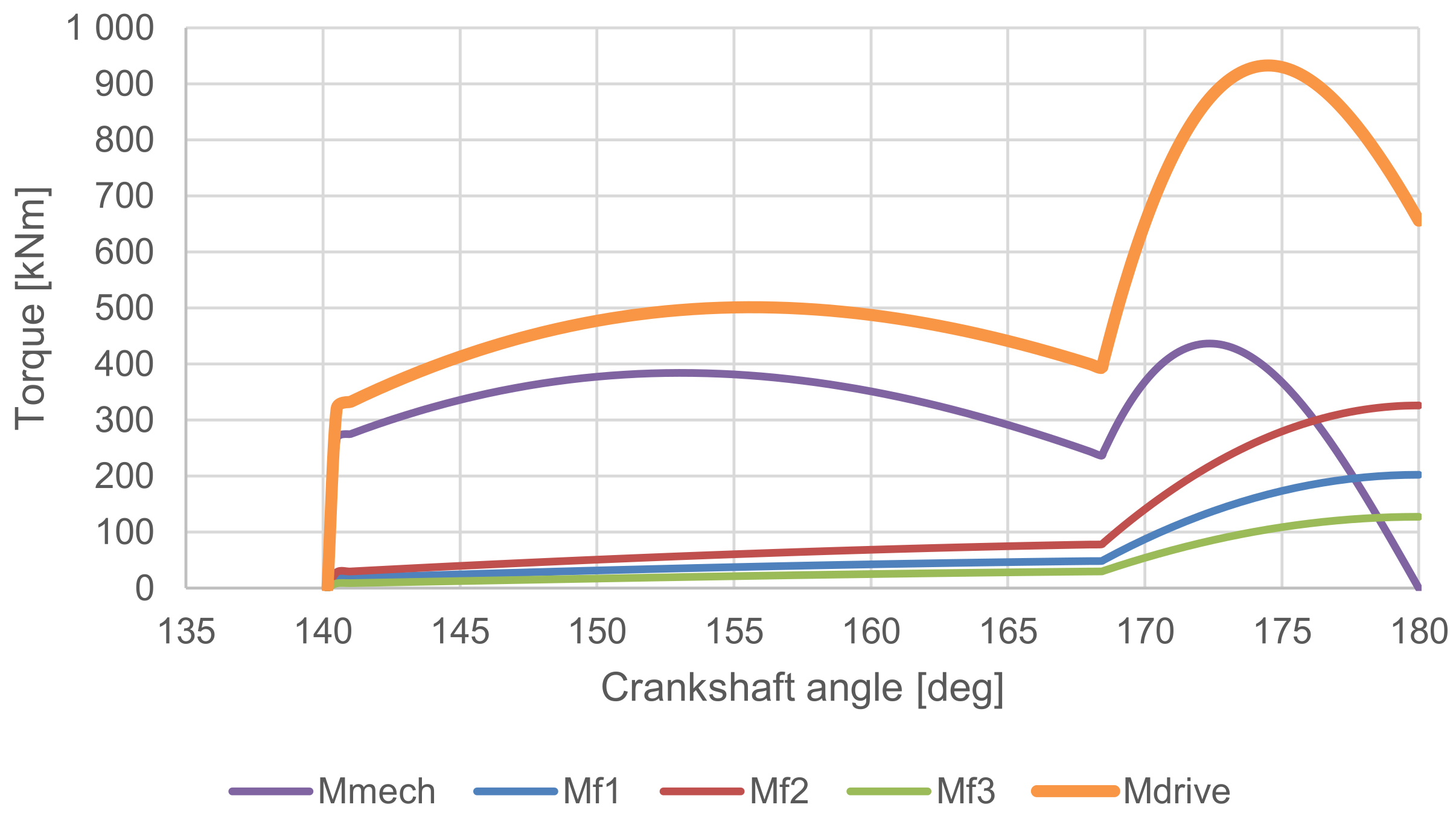
The graph on Figure 9 shows the torque results of analytical dynamic calculation. Shapes of these torque curves are similar to those from the previous calculation approach.

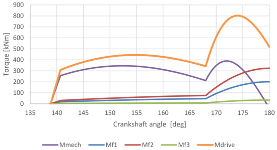
Figure 9. The graph of torques versus crankshaft angle—Analytical Dynamic Calculation.

The final friction values obtained through analytical calculation are presented in Table 6.

7. Multibody Simulation of Press Mechanism

Multibody simulation (MBS) is a numerical simulation method that employs rigid or elastic bodies connected by various kinematic constraints or force elements. Unilateral constraints, such as contacts, may be accompanied by Coulomb friction models, among other possibilities. Ultimately, it is a highly effective tool for investigating, optimising, and verifying machine mechanisms. To investigate the friction qualities of a press mechanism, MSC Adams/View software was employed.

For the computational model to calculate the state vector, it was necessary to compile the equations of motion and constraints. These equations then formed three systems of nonlinear algebraic and differential equations [15], which were composed in the background by the software and then processed by the solver. The systems consisted of the following equations:

• Six first-order equations for the dynamic behaviour of each part of the model (connecting forces to accelerations).
• Six first-order equations for the kinematic behaviour of each part of the model (connecting forces to velocities).
• One algebraic equation for each motion constraint.
• One algebraic equation each scalar force component.
• Arbitrary number of user-added algebraic or first-order differential equations.

Subsequently, the system generated a solution in accordance with the underlying mathematical equations.

$$\begin{array}{c}\mathit{M}\left(\mathit{q},\mathit{u},\dot{\mathit{u}},\mathit{f},t\right)=0\\ \mathit{u}-\dot{\mathit{q}}=0\\ \mathsf{\Phi }\left(\mathit{q},\mathit{f},t\right)=0\end{array}$$

(19)

where $\mathit{M}$ is a column vector representing all differential equations describing the dynamics of the model and the user-added differential equations. Symbol $\mathit{q}$ marks the generalized coordinates of displacement and rotation, and symbol $\mathit{u}$ marks the time derivatives of generalized coordinates, which corresponds to the second system of equations. The third system of equations contains column vector $\mathit{\Phi }$, which contains algebraic constraint equations [16].

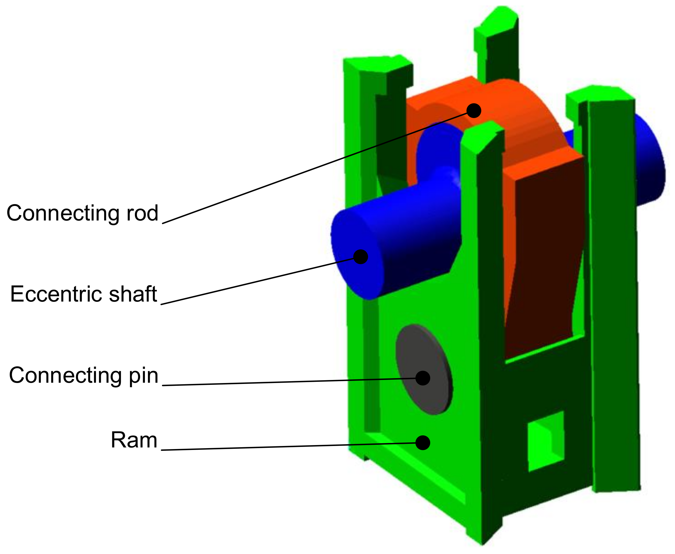
The crank press model comprises four principal components as follows: the eccentric shaft, the connecting rod, the connecting pin, and the ram. These components are interconnected by joints that eliminate the corresponding degrees of freedom (DOFs). The eccentric shaft is connected to the ground through a revolute joint, thereby enabling the shaft to rotate about its main axis. Subsequently, a revolute joint is applied to the eccentric shaft and connecting rod. Subsequently, the connecting rod is linked by a further revolute joint to the connecting pin, which is then secured to the ram. The ram is attached to the ground through a translational joint.

The initial conditions of multibody simulation are as follows (Table 7):

Table 7. The initial conditions of Multibody Simulation.

	Status
Rigid body mechanism	rigid
Angular velocity of the crankshaft	constant
Inertial forces	included
Gravitational acceleration	included
Weight balancing	neglected

The initial conditions were identical to those employed in previous calculation approaches. This enabled a direct comparison of the results of these calculations. In addition to the geometric and inertia properties of the press mechanism (Figure 10 and Figure 11), the initial conditions included the angular speed of the crankshaft.

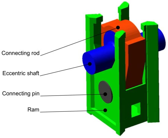
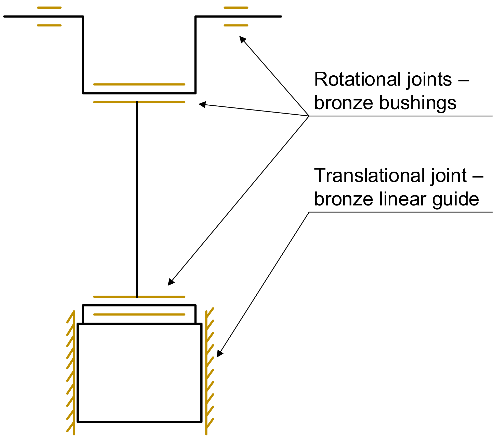
Figure 10. Description of press mechanism parts in multibody model.

Figure 11. Schematic description of body joints in multibody model.

The simulation of the mechanism was conducted for the entirety of the work stroke. Consequently, the crankshaft rotated by 360°, rather than merely by 41.28° to the BDC.

As a consequence, it was possible to compare the friction energy losses of the entire work stroke with those generated during the forging phase of the stroke. The subsequent graphs illustrate the relationship between friction torque and friction work, as a function of crankshaft angle. As previously stated, the friction work is an integral component of the friction torque.

Results of MBS

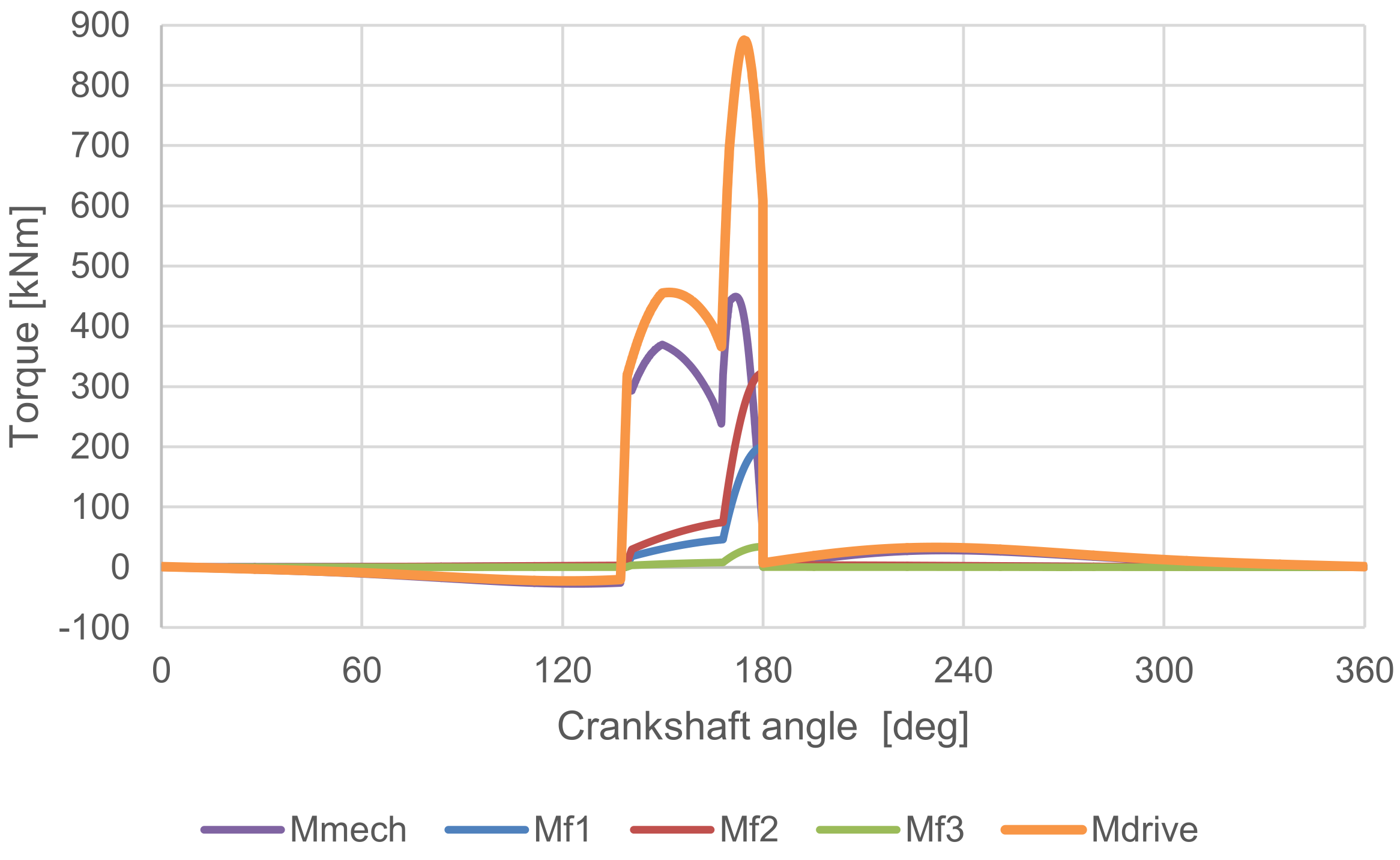
The results of the MBS simulation are presented in Figure 12, which depicts the relationship between torque and crankshaft angle. The crankshaft angle is represented by a full 360°, encompassing the entirety of the work stroke. This enabled us to observe how the driving torque Mdrive was affected by gravity. In the portion of the cycle beginning at the top dead centre (TDC), the gravitational force acted in a downward direction on the ram, resulting in a negative driving torque. Following the completion of the technological operation, the driving torque remained at non-zero, as it was necessary to pull the ram up to the TDC once more.

Figure 12. The graph of torques versus the crankshaft angle for the whole work stroke.

Also, the final friction works are similar enough to previous calculation approach. One advantage of the MBS simulation is the ability to obtain the values for the entire work stroke (Table 8).

Table 8. The results of Analytical Dynamic Calculation.

	AMech	Af1	Af2	Af3	Az	ADrive
	kJ
MBS simulation—forging	224	51	82	9	142	381
MBS simulation—whole stroke	224	56	86	9	151

8. Summary and Commentary of the Results

Table 9 presents the resulting values of friction losses obtained by all the calculation approaches.

Table 9. Overall results of friction losses calculations.

	AMech	Af1	Af2	Af3	Az	ADrive
	kJ
Empiric	220	n/a	n/a	n/a	(176 ÷ 220) For a press with a flexible stand!	396 ÷ 440
Calculation in a Spreadsheet	224	50	82	9	141	364
Analytical Dynamic Calculation	224	50	81	9	140	376
MBS simulation—forging	224	51	82	9	142	381

The results of the Empirical Method diverged significantly from those of the other methods (the expected value of friction work was higher). This discrepancy can be attributed to the fact that the friction work was monitored on a real machine, which is inherently flexible, in contrast to a rigid machine. The elastic deformation of the machine during the forging phase of the stroke results in the necessity to perform a larger angle of rotation of the crankshaft in order to achieve the desired deformation of the forged blank. This results in a greater friction torque and greater angle and thus greater frictional work. In the case of a flexible machine, it is also necessary to consider the spring-load of the machine after the BDC has been overcome, i.e., further friction work.

The outcomes of the Spreadsheet calculation, Analytical Dynamic Calculation, and MBS Simulation (forging) were found to be largely consistent, thereby confirming their accuracy. The results of the Analytical Dynamic Calculation and MBS Simulation were the most similar, with the values of friction work being lower when compared to the Spreadsheet approach. This discrepancy can be attributed to the fact that the Spreadsheet does not account for the influence of gravity, which exerts a force on the internal components of the mechanism.

A significant outcome of comparing the outcomes of disparate calculations was the validation of their precision. The equality of the results of the Spreadsheet Calculation and the MBS Simulation indicates that the kinetostatic approach employed was valid. For future simulations, the MBS simulation can be relied upon, as it offers possibilities that are not achievable with the Spreadsheet calculation.

9. The Following Research Proposal

A comparison of the results of the calculations with those derived through Empirical Method revealed that the effect of machine spring-load was not negligible. Consequently, the subsequent step would be to incorporate the spring into the calculation.

Given that the desired outcome is a reduction in friction energy, which is directly proportional to the friction coefficient, it is possible to extend the simulations by considering the influence of other parameters on the friction coefficient. It can be postulated that the friction loss may be influenced by alterations to the lubrication of the machine.

It is assumed that the MBS simulation will continue to be employed, as it is compatible with the 3D solids that are currently available, given that these are also utilised in other simulations. Furthermore, the effect of weight counterbalancing should be incorporated into the simulation, and the friction losses can then be monitored throughout the entire stroke, rather than solely during the forming operation, as observed in this paper. Furthermore, the effect of the crankshaft angular velocity, dependent on the consumption of energy accumulated in the flywheel during the stroke, including clutch engagement, can be included in the calculation.

The subsequent objective of the mechanical press simulation would be to ascertain the dynamic effects of its operation on its surroundings.

References

- Brabec, P.; Voženílek, R.; Menič, B. Crankshaft Mechanism with Offset for the Combustion Engine. In Engineering Mechanics 2019, Proceedings of the 25th International Conference, Svratka, Czech Republic, 13–16 May 2019; Institute of Thermomechanics of the Czech Academy of Sciences: Prague, Czech Republic, 2019; pp. 65–68. [Google Scholar] [CrossRef]
- Quinci, F.; Litwin, W.; Wodtke, M.; van den Nieuwendijk, R. A comparative performance assessment of a hydrodynamic journal bearing lubricated with oil and magnetorheological fluid. Tribol. Int. 2021, 162, 107143. [Google Scholar] [CrossRef]
- Dindorf, R.; Wos, P. Energy-Saving Hot Open Die Forging Process of Heavy Steel Forgings on an Industrial Hydraulic Forging Press. Energies 2020, 13, 1620. [Google Scholar] [CrossRef]
- Jiao, R.; Nguyen, V. Study on Lubrication Efficiency and Friction Power Loss of Engine Based on a Hybrid Hydrodynamic Model. Int. J. Automot. Mech. Eng. 2021, 18, 8859–8869. [Google Scholar] [CrossRef]
- Hailemariam, N. 2015 Kinematics and Load Formulation of Engine Crank Mechanism. Mech. Mater. Sci. Eng. 2015, 1, 2412–5954. [Google Scholar]
- Bucciarelli, L.L. 3 Internal Forces and Moments. In Engineering Mechanics for Structures; Dover Publications: Mineola, NY, USA, 2019; pp. 53–104. Available online: https://ocw.mit.edu/courses/1-050-solid-mechanics-fall-2004/resources/emech3_04/ (accessed on 14 January 2022).
- Stribeck, R. Kugellager für beliebige Belastungen; Springer: Berlin/Heidelberg, Germany, 1901. [Google Scholar]
- Razavykia, A.; Delprete, C.; Baldissera, P. Numerical Study of Power Loss and Lubrication of Connecting Rod Big-End. Lubricants 2019, 7, 47. [Google Scholar] [CrossRef]
- Tormos, B.; Martín, J.; Carreño, R.; Ramírez, L. A general model to evaluate mechanical losses and auxiliary energy consumption in reciprocating internal combustion engines. Tribol. Int. 2018, 123, 161–179. [Google Scholar] [CrossRef]
- Bele, M.; Hlavac, J. Evaluation of the Energy Intensity of Forming Machines Compared to Approaches in Other Industries. In Proceedings of the 28th International DAAAM Symposium, Zadar, Croatia, 8–11 November 2017; pp. 1057–1064. [Google Scholar] [CrossRef]
- Rudolf, B.; Kopecký, M. Tvářecí Stroje—Základy Stavby a Využití (Forming Machines—Basics of Construction and Use); SNTL: Prague, Czech Republic, 1985. [Google Scholar]
- Kríž, Z.; Švandová, V. Numerická Integrace. pp. 1–6. Available online: https://is.muni.cz/el/sci/jaro2017/C2140/um/ch07.pdf (accessed on 14 January 2022).
- Beer, F.; Johnston, E.; Mazurek, D.; Cornwell, P. Vector Mechanics for Engineers: Statics and Dynamics, 11th ed.; McGraw Hill: New York, UK, USA, 2015. [Google Scholar]
- The MathWorks, Inc. Fsolve; The MathWorks, Inc.: Natick, MA, USA; Available online: https://www.mathworks.com/help/optim/ug/fsolve.html (accessed on 18 September 2022).
- Marques, F.; Rychecký, D.; Isaac, F.; Hajžman, M.; Polach, P.; Flores, P. Spatial Revolute Joints with Clearance and Friction for Dynamic Analysis of Multibody Mechanical Systems. In Proceedings of the 4th Joint International Conference on Multibody System Dynamics, Montreal, QC, Canada, 31 May 2016; pp. 1–10. [Google Scholar]
- Adams Solver User’s Guide [online]. Adams 2021.2. MSC Software Corporation. 2021. Available online: https://nexus.hexagon.com/documentationcenter/cs-CZ/bundle/Adams_2021.2_Adams_Solver_User_Guide/resource/Adams_2021.2_Adams_Solver_User_Guide.pdf (accessed on 3 November 2022).
Disclaimer/Publisher’s Note: The statements, opinions and data contained in all publications are solely those of the individual author(s) and contributor(s) and not of MDPI and/or the editor(s). MDPI and/or the editor(s) disclaim responsibility for any injury to people or property resulting from any ideas, methods, instructions or products referred to in the content. |
© 2024 by the authors. Licensee MDPI, Basel, Switzerland. This article is an open access article distributed under the terms and conditions of the Creative Commons Attribution (CC BY) license (https://creativecommons.org/licenses/by/4.0/).