Prediction and Dynamic Simulation Verification of Output Characteristics of Radial Piston Motors Based on Neural Networks

Abstract

Radial piston motors are executive components in hydraulic systems, tasked with providing appropriate torque and speed according to load requirements in practical applications. The purpose of this study is to predict the output torque of radial piston hydraulic motors and confirm their suitable operating conditions. Efficiency determination experiments were conducted on physical models, yielding thirty sets of performance data. Torque (output torque) and mechanical efficiency from the experimental data were selected as prediction targets and fitted using two methods: multiple linear regression and neural networks. A dynamic simulation model was built using Adams2020 software to obtain theoretical torque values, enabling the verification of the alignment between the predicted values and simulation results. The results indicate that the error between the theoretical torque of the dynamic model and the physical experiments is 1.9%, with the error of the neural network predictions being within 2%. The dynamic simulation model can yield highly accurate theoretical torque values, providing a reference for the external load of hydraulic motors; additionally, neural networks offer accurate predictions of output torque, thus reducing experimental testing costs.

1. Introduction

Hydraulic systems are widely used in engineering and industrial applications today, playing a crucial role in power transmission and motion control for heavy machinery and processing equipment. Hydraulic motors are essential components within hydraulic transmission systems, and their working principle is similar to that of hydraulic pumps. Hydraulic pumps need to provide a certain flow rate and pressure to the hydraulic system to meet its energy demands, with a greater emphasis on volumetric efficiency. In contrast, hydraulic motors typically need to provide appropriate torque and speed according to workload requirements, placing a higher emphasis on the output efficiency. Current research primarily focuses on aspects such as the contact surface friction performance, internal fluid characteristics, torque output, and structural optimization.

In the research on friction performance, numerous studies have indicated that a better tribological performance and reduced wear can be achieved by altering the surface texture within hydraulic motors [1,2,3]. Bingjing Qiu et al. [4] investigated the influence of different materials on the friction performance under low-speed, high-pressure conditions. Fei LYU et al. [5] utilized finite element methods to study the wear between the pistons and cylinder barrel of an axial piston pump, elucidating the real-time interaction mechanisms between cylinder liner wear and the bearing and lubrication conditions during the wear process. L. Ceschini et al. [6] conducted bench tests and laboratory dry sliding tests on boundary-lubricated sliding contact components of radial piston hydraulic motors, investigating the tribological performance of radial piston hydraulic motors.

Research on the fluid characteristics of hydraulic motors includes Zhiqiang Wang et al. [7], who conducted a study on seawater hydraulic motors, investigating the effects of water film, inlet pressure, and speed on the pressure distribution and leakage of the valve plate; Piotr Patrosz [8] examined the influence of the fluid properties within axial piston pumps on the peak chamber pressure; Lingxiao Quan et al. [9] investigated the fluid dynamic evolution process of the valve plates in axial piston pumps, analyzing the vortices of different scales, intensities, and positions generated during the valving process; and Pawel Sliwinski et al. [10] employed computational fluid dynamics (CFD) to test pressure losses of water and mineral oil in motors, proposing a novel method for measuring internal channel pressure losses within the motor.

Regarding the torque output of motors, Venkata Harish Babu Manne et al. [11] proposed a method to evaluate torque efficiency by assessing an instantaneous pressure rise in each displacement chamber using a lumped parameter approach. Yueyue Nie et al. [12] validated motor low-speed characteristics through AMESim software. Yinshui Liu et al. [13] studied the torque efficiency of motors in deep-sea environments using finite element analysis software. Pawel Sliwinski et al. [14] further elucidated the relationship between the motor input flow and speed under stable pressure differential conditions.

Research on structural optimization includes Guangjun Liu et al. [15] who proposed a multidisciplinary design optimization method for swash plate axial piston pumps based on collaborative simulations and integrated optimization. Studies on flow pulsation, vibration characteristics, cavitation phenomena, and speed pulsation during motor operation have led to the proposal of structural optimization schemes [16,17,18,19,20].

In other areas, valuable research exists. Hui Shen et al. [21] established a dynamic model of axial piston pumps to study piston motion under different conditions, analyzing the effects of the hydraulic pressure, piston radius, and radial clearance on the forward displacement, contact radius, maximum contact pressure, and other aspects. Junhui Zhang et al. [22] proposed a neural network model for assessing noise in axial piston pumps. Gautham Ramchandran et al. [23] investigated a novel numerical method to simulate the physical processes of piston operation within radial piston pumps. Daniel Nilsson et al. [24] conducted extensive testing on hydraulic motor extreme conditions, presenting three stages of motor stalling. Lifu Cheng et al. [25] compared the fatigue characteristics of composite materials and high-strength structural steel, confirming that composite materials can replace traditional steel in hydraulic motors.

In summary, significant achievements have been made in various aspects of research on hydraulic pumps and hydraulic motors. The research on dynamic simulations mainly focuses on analyzing the operation of internal components during motor operation. This paper aims to determine the theoretical torque of the motor using dynamic simulation methods. First, the operating data of the radial piston motor are measured through physical experiments. Next, the experimental data are fitted using neural networks to predict the output under the different operating conditions of the motor. Then, a simulation model is constructed and the theoretical torque feedback from the simulation model is compared with the experimentally measured data to demonstrate the reliability of the simulation results. Furthermore, the simulation model is used to verify the data predicted by the neural network. Finally, the main findings of the research project are summarized and conclusions are drawn.

2. Torque for the Radial Piston Motor

2.1. Structure of the Radial Piston Motor

As shown in Figure 1, the radial piston motor is mainly composed of components such as the Rear cover, Rear housing, Stator, Motor mount, Plunger, Roller, Distribution plate, and Rotor. The stator guide rail of the motor is fixed to the motor mount and the distribution plate and motor mount form the internal flow passages of the motor. The flow from the hydraulic system drives the rotor to rotate, with ten plungers positioned within the ten plunger chambers on the rotor. The rollers are fitted to the outer ends of the plungers and run closely against the inner side of the stator during operation.

When high-pressure hydraulic fluid is delivered to the hydraulic motor, it flows into the motor’s plunger chambers through the high-pressure oil port on the rear housing. Acting on the bottom of the plungers, it propels the plungers outward, causing them to move radially in a reciprocating motion within the curves of the stator guide rail. At the other end of the plunger, rollers are fitted, which, upon contact with the inner side of the stator guide rail, generate tangential force, driving the spindle associated with the hydraulic motor into rotational motion. This rotational motion can be utilized to drive various loads such as windmills, hydraulic robotic arms, conveyor belts, and so forth.

2.2. Force Analysis between the Roller and the Stator Guide Rail

The interaction between the roller and the stator guide rail is illustrated in Figure 2. In the figure, ρ is the distance from the center of the roller to the center of rotation of the rotor and p is the hydraulic pressure acting outward along the axis of the plunger under the action of hydraulic fluid. This force is divided into two components at the contact between the roller and the guide rail: F_N and F_T. F_N is the normal pressure perpendicular to the contact surface between the roller and the guide rail, where β is the angle between p and F_N. F_T is the tangential force that drives the rotation of the rotor.

The angle β changes continuously as the rotor rotates. The instantaneous magnitude of the tangential force F_T can be expressed as:

$$F_T=p·\tan \beta$$

(1)

The product of F_T [N] and ρ [m] gives the instantaneous theoretical torque of the plunger at the current position. For the radial piston motor studied in this research, which has ten plungers, the theoretical torque during operation can be expressed through mechanical analysis as:

$$M_R=\mathsf{\Delta }P{\displaystyle \sum _{\mathrm{i}=1}^{\mathrm{z}}{\rho }_{\mathrm{i}}}\tan {\beta }_{\mathrm{i}}$$

(2)

where M_R [N·m] is the instantaneous torque, ΔP [N] is the pressure difference between the inlet and outlet of the motor, ρ_i [m] is the moment arm of roller i, and z = 10 denotes ten rollers.

3. Hydraulic Motor Efficiency Testing Experiment

The motor efficiency testing experiment has three primary purposes: 1. Determine the actual output torque and mechanical efficiency of the motor under different operating conditions. 2. Provide data support for evaluating the motor’s applicable operating conditions by testing its performance under various conditions. 3. Verify if the motor can operate smoothly.

3.1. Introduction to the Experiment

In this experiment, for the radial piston motor, it is crucial to ensure the presence of back pressure in the return oil pipeline. When the piston returns, the absence of pressure in the piston chamber can cause the piston and roller to disengage from the stator guide surface due to inertial effects, leading to cavitation or impact. Moreover, this phenomenon intensifies with the increasing speed.

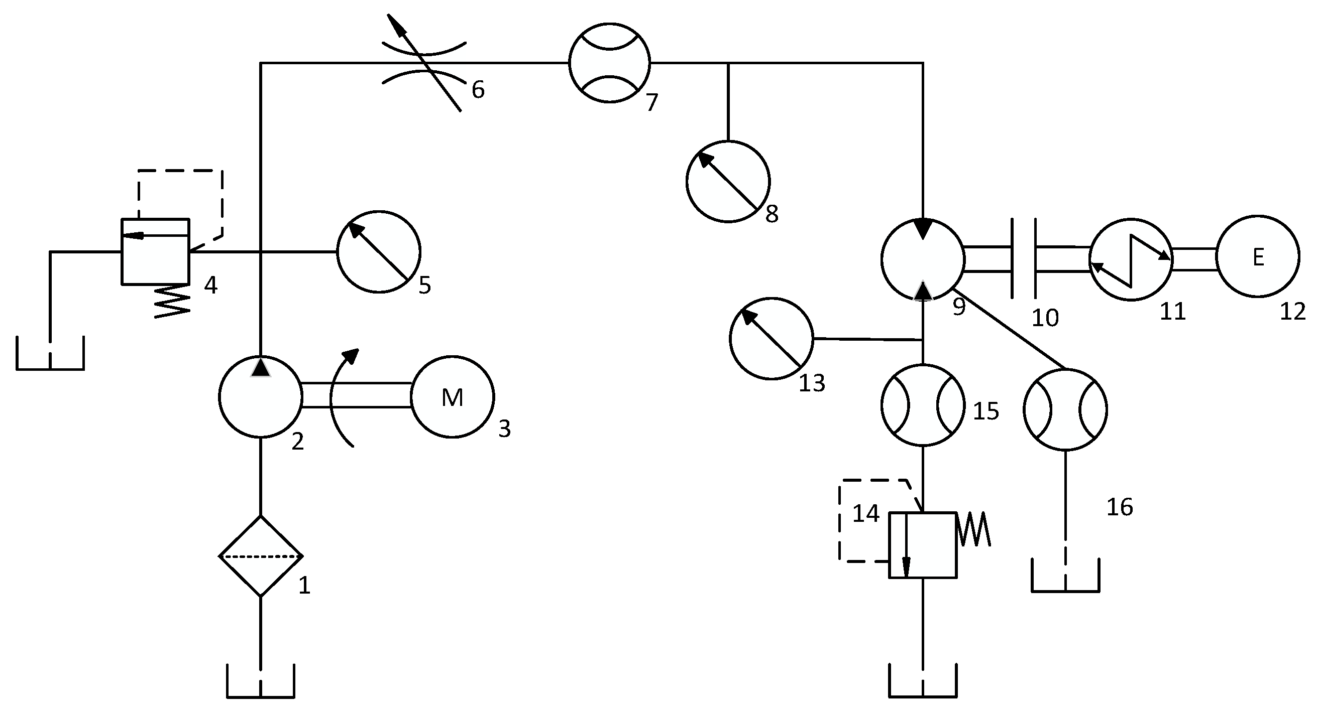
The experimental hydraulic system operates as illustrated in Figure 3. The hydraulic pump (2) is responsible for extracting fluid from the reservoir and boosting its pressure to generate sufficient flow and pressure to drive the actuator. In this experiment, the hydraulic system is powered by motor (3), and hydraulic pump (2) delivers fluid through filter (1) into the hydraulic pipeline. Overflow valves (4) and (14) serve as pressure control valves for regulating the inlet and outlet pressures of the hydraulic motor. The throttle valve (6) controls the input flow to the motor, thereby controlling the motor’s output speed. Flow meters (7) and (15), respectively, measure the input flow and return flow of the motor, with the motor’s leakage being the difference between the two. The experiment employs a load motor as a loading device to simulate different torque and speed conditions accurately, with torque sensors used to measure the output torque.

Figure 4 depicts the experimental testing setup. The no-load displacement of the hydraulic motor in this experiment is calculated as 1350 cc. The primary parameters to be recorded in this experiment include the hydraulic fluid pressure at the inlet and outlet of the hydraulic motor, the output torque, the total fluid intake, and the return fluid flow.

3.2. Experiment Data

In the hydraulic motor efficiency testing experiment, “Total fluid intake” refers to the volumetric flow rate of liquid entering the motor per unit of time, which is the actual flow rate Q_S [cm³/s]. The flow rate required for the internal sealing chamber variations of the motor is termed as the theoretical flow rate Q_L [cm³/s], which in the experiment, refers to the return fluid flow. The leakage flow rate is the motor’s leakage quantity ΔQ [cm³/s].

$$\mathsf{\Delta }Q=Q_s-Q_L$$

(3)

The volumetric efficiency (ŋ_v) of a hydraulic motor is the ratio of the theoretical input flow rate Q_L (return fluid flow) to the actual input flow rate Q_S (total fluid intake).

$${\eta }_v={\displaystyle \frac{Q_L}{Q_S}}$$

(4)

Due to motor leakage, when calculating the actual speed n [rps] using the actual fluid flow rate Q_S, the volumetric efficiency should be taken into account.

$$n={\displaystyle \frac{Q_S}{q}}{\eta }_v$$

(5)

where Q_S is the actual flow rate and q [mL/r] is the motor displacement (1350 mL/r).

The output torque (M_S) of a hydraulic motor is measured against an external load. For a hydraulic system, the theoretical torque (M_L) of the hydraulic motor can be determined from the perspective of energy conservation.

$$M_{L}2\pi n=\mathsf{\Delta }p{Q}_S=\mathsf{\Delta }pqn$$

(6)

$$M_L={\displaystyle \frac{\mathsf{\Delta }pq}{2\pi }}$$

(7)

where M_L [N·m] is the theoretical torque of the hydraulic motor and Δp [Mpa] is the pressure difference between the inlet and outlet of the hydraulic motor.

The mechanical loss of a hydraulic motor refers to the energy loss caused by the relative movement between the internal components of the hydraulic motor and the friction between the fluid and the components. This loss results in a reduction in the actual output torque.

$$M_S=M_L-\mathsf{\Delta }M$$

(8)

where ΔM [N·m] is the torque loss caused by friction, and M_S [N·m] refers to the actual output torque measured in the hydraulic motor experiment.

Mechanical efficiency (ŋ_m) can be described as the ratio between the actual output torque and the theoretical output torque of a hydraulic motor during operation.

$${\eta }_m={\displaystyle \frac{M_S}{M_L}}$$

(9)

The experiment controlled the hydraulic motor speed by controlling the hydraulic system flow rate. Data were collected for the motor’s operation under five different speed conditions: 20 rpm, 40 rpm, 60 rpm, 80 rpm, and 90 rpm.

$${\eta }_m={\displaystyle \frac{2\pi M_S}{q\mathsf{\Delta }p}}\times 100\%$$

(10)

where M_S [N·m] is the actual torque measured in the experiment and q is the motor displacement, taken as 1350 mL/r.

The experimental data are presented in

Table 1. Experimental Data for Hydraulic Motor Efficiency Measurement.

Serial Number	Inlet Pressure/MPa	Outlet Pressure/MPa	Pressure Difference/MPa	Speed/rpm	Torque/N·m	Mechanical Efficiency/%	Total Inflow L/min	Return Flow L/min	Volumetric Efficiency/%
1	4.35	0.31	4.04	19	640	73.69	26.825	26.3	95.62
2	6.35	0.32	6.03	20	991	76.45	29.355	28.8	91.98
3	8.35	0.31	8.04	20	1348	77.99	29.715	28.5	90.86
4	10.35	0.31	10.04	20	1697	78.63	29.8	28.3	90.60
5	15.4	0.3	15.1	19.5	2590	79.79	29.93	27.8	87.96
6	18.3	0.31	17.99	19.5	3097	80.08	30.2	27.5	87.17
7	4.47	0.44	4.03	41	542	62.56	57.82	57.1	95.73
8	6.45	0.45	6	41	895	69.39	58.24	57.1	95.04
9	8.47	0.46	8.01	41	1249	72.54	58.85	57.2	94.05
10	10.47	0.44	10.03	41.5	1598	74.11	59	57.2	94.96
11	15.45	0.44	15.01	41.5	2463	76.33	60.6	58.2	92.45
12	18.45	0.44	18.01	42	2959	76.43	61.14	58.2	92.74
13	4.74	0.6	4.14	60.5	383	43.04	83.9	83	97.35
14	6.7	0.56	6.14	58.5	764	57.88	81.83	80.6	96.51
15	8.78	0.58	8.2	61.5	1098	62.29	86.3	84.8	96.21
16	10.68	0.59	10.09	61.5	1437	66.25	86.95	84.85	95.49
17	15.53	0.6	14.93	62	2249	70.07	88.9	86.2	94.15
18	18.54	0.6	17.94	62	2769	71.80	90	86.7	93.00
19	4.81	0.77	4.04	81	141	16.24	111.7	110.5	97.90
20	6.97	0.78	6.19	81	520	39.08	113	111.5	96.77
21	8.75	0.78	7.97	81	832	48.56	113.23	111.4	96.57
22	10.7	0.78	9.92	81	1171	54.91	113.4	111	96.43
23	15.6	0.77	14.83	79	2037	63.90	111.7	108.7	95.48
24	18.55	0.75	17.8	77.5	2550	66.64	110.4	107.1	94.77
25	4.87	0.83	4.04	89	73	8.41	122.49	121.2	98.09
26	6.79	0.81	5.98	86.5	448	34.85	119.45	118.1	97.76
27	8.58	0.78	7.8	84.5	783	46.70	117.53	115.7	97.06
28	10.8	0.77	10.03	82.5	1189	55.15	115.5	113.1	96.43
29	15.51	0.74	14.77	79.5	2045	64.41	112.8	109.8	95.15
30	18.58	0.73	17.85	77.5	2588	67.45	110.8	107.2	94.43

.

4. Output Characteristics Prediction

The radial piston motor in this study uses a face distribution structure. At low rotational speeds, the fluid cannot maintain the sealing state of the motor’s face distribution, resulting in relatively large internal leakage. Under the same rotational speed conditions, as the inlet pressure increases, the volumetric efficiency decreases. As shown in Table 1, the motor’s volumetric efficiency remains relatively stable under different hydraulic system input conditions.

The input conditions of the hydraulic system significantly affect the motor’s output torque and mechanical efficiency. This study uses two methods, linear regression and neural networks, to fit the existing experimental data and predict the motor’s output under different operating conditions.

4.1. Regression Analysis

The main input conditions of the hydraulic system include the inlet pressure, outlet pressure, and flow rate. Multiple linear regression requires the independent variable data to be mutually independent, so a correlation analysis can be performed first to select the independent variables. Considering the relationship between torque and inlet pressure, this study attempts to use mechanical efficiency as the dependent variable and the input conditions from the experimental data as independent variables. Multiple linear regression is then used to fit the mechanical efficiency.

4.1.1. Correlation Analysis

Lacking an understanding of the degree of correlation and the possible association patterns among experimental variables, IBM SPSS Statistics 24 data analysis software can be used to perform a correlation analysis on the experimental data. This in-depth analysis helps to uncover the intrinsic relationships between the experimental data. Through correlation analysis, it is possible to determine whether there are linear or nonlinear relationships between these variables, as well as the strength and direction of these relationships.

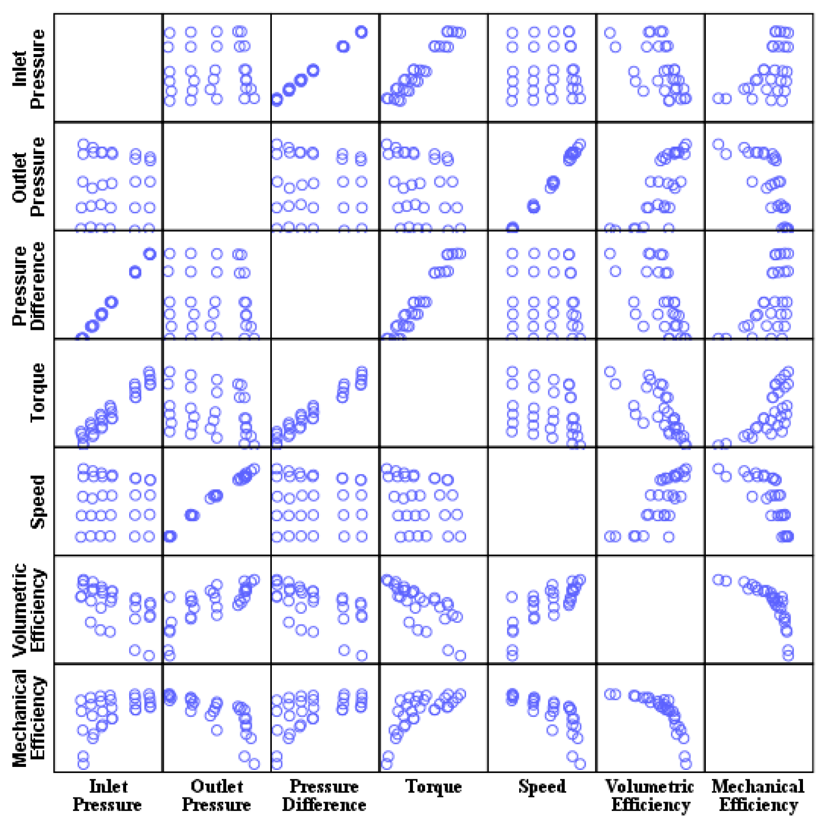
Figure 5 is a matrix scatter plot, showing a linear positive correlation between the speed and outlet pressure. This adjustment in outlet pressure at each speed test point is to prevent issues such as clearance and impact between plungers and rollers as the speed increases. There is a clear positive correlation between the output torque and inlet pressure. However, there is no apparent linear relationship between the mechanical efficiency and other parameters. Selecting mechanical efficiency as the dependent variable is more appropriate in this case.

When selecting the correlation coefficient, the Pearson correlation coefficient should be chosen, and for significance testing, a two-tailed test should be selected. The Pearson correlation coefficient is a statistical measure used to assess the linear relationship between two variables, with values ranging from −1 to 1. A correlation coefficient of 1 indicates a perfect positive correlation, while a correlation coefficient of −1 indicates a perfect negative correlation.

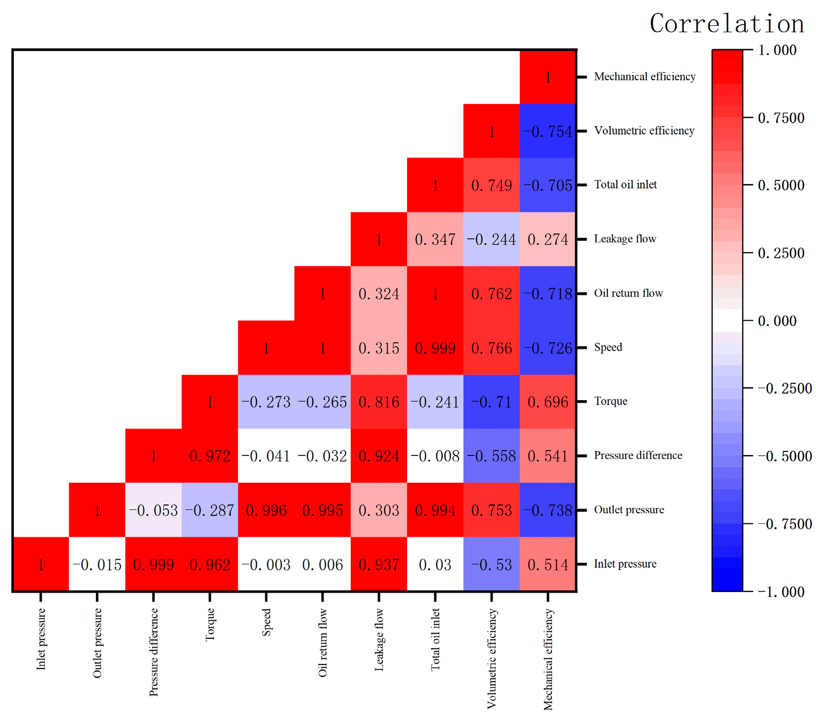
The correlation heatmap in Figure 6 illustrates the strengths of the relationships between experimental parameters. The speed of the hydraulic motor is controlled by the system flow rate, which depends on the return oil flow rate, resulting in a correlation coefficient of 1. The inputs to the hydraulic system, including the inlet pressure, outlet pressure, speed, and flow rate, do not exhibit strong correlations with the mechanical efficiency of the hydraulic motor (correlation coefficients are below 0.90).

4.1.2. Multiple Linear Regression

Based on the information provided by the matrix scatter plot and the correlation heatmap, it is essential to avoid multicollinearity issues when selecting independent variable parameters. The selection of independent variables should be adjusted according to the R² value, significance, Durbin–Watson value (DW test for autocorrelation), collinearity statistics (VIF test for collinearity), and residual distribution feedback from the software in the linear regression results. After several attempts, when the number of independent variables is set to three, choosing the pressure difference, external leakage flow, and return oil flow results in a relatively ideal regression model.

The R² value of 0.807 in

Table 2. Model Summary.

R	R2	Adjust R2	Standard Estimate of Error	Durbin–Watson
0.898	0.807	0.785	8.43592	1.778

indicates that the selected independent variables account for approximately 80.7% of the variation in mechanical efficiency when subjected to multivariate regression. The Durbin–Watson statistic is used to test for autocorrelation. An ideal range for this statistic is between 1.97 and 2.03. Values within the range of 1.5 to 2.5 are considered acceptable.

Table 3. Mechanical Efficiency Coefficient.

Model Parameters	Unstandardized Coefficients		Standardized Coefficients	t	Significance	Collinearity Statistics
	B	Standard Error	Beta			Tolerance	VIF
Constant	82.052	7.782		10.544	0.000
Pressure Difference	−1.602	2.043	−0.436	−0.784	0.440	0.024	41.549
Leakage Flow	21.431	12.323	1.021	1.739	0.094	0.022	46.371
Return Flow Rate	−0.581	0.123	−1.062	−4.729	0.000	0.147	6.798

provides the regression model coefficients. From these coefficients, we can derive the linear regression equation for mechanical efficiency with respect to three parameters: pressure difference (Δp), external leakage flow (ΔQ), and return oil flow (Q_L).

$${\eta }_m=82.052-1.602\mathsf{\Delta }p+21.431\mathsf{\Delta }Q-0.581Q_L$$

(11)

The Variance Inflation Factor (VIF) is a metric used to assess the degree of multicollinearity among the independent variables in a linear regression model.

4.2. Multi-Layer Perceptron (MLP)

We decided to train a neural network model to learn the mapping relationship from input features to output targets. During this process, the model adjusts its Weights and Thresholds iteratively to minimize the difference between the predicted output and the true target. The operational flow of the neural network is shown in Figure 7.

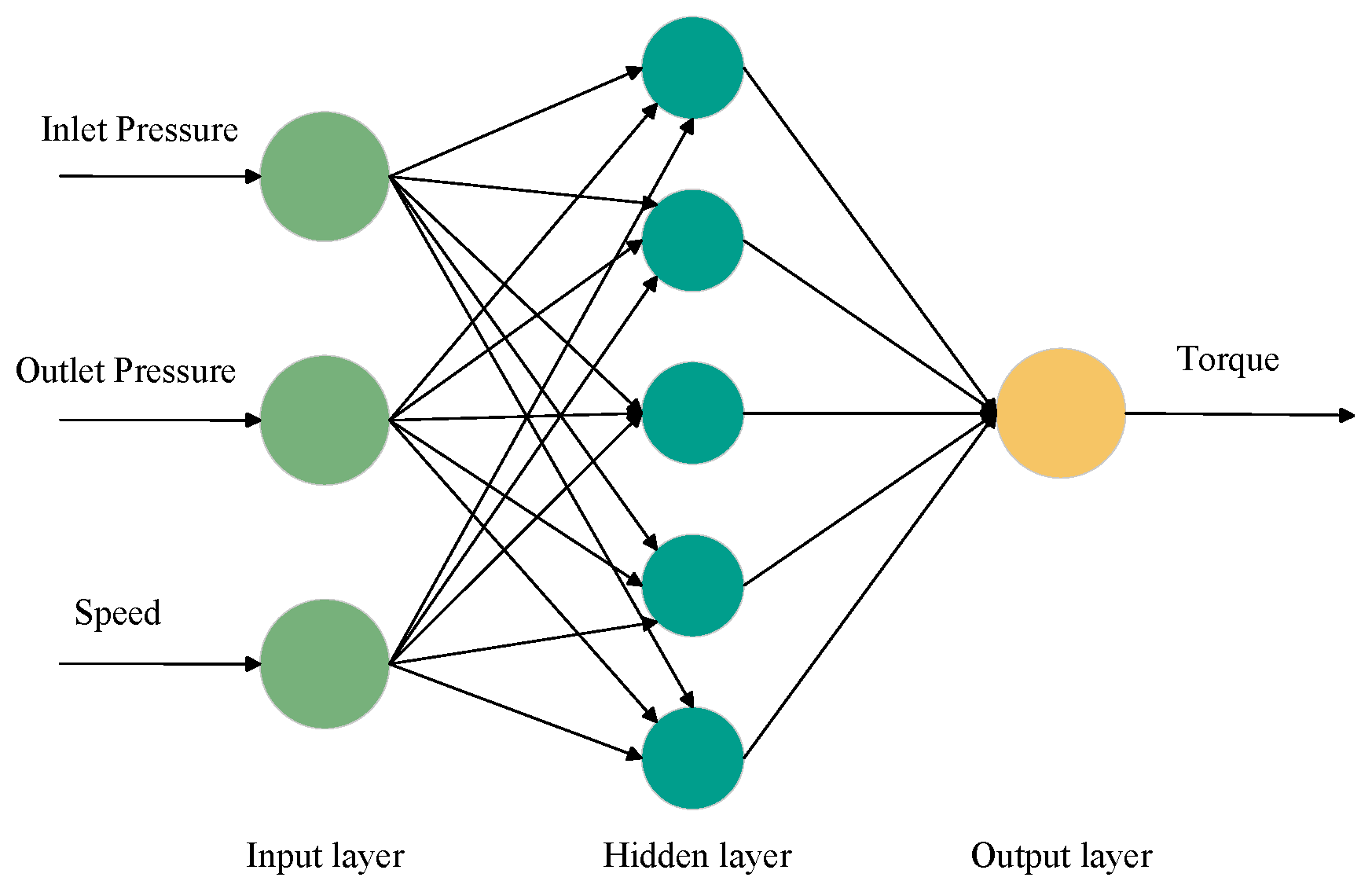
Considering the potentially complex nonlinear relationships among the experimental parameters, a Multi-Layer Perceptron (MLP) neural network is used here for data fitting. The neural network architecture is shown in Figure 8.

The hydraulic system flow rate controls the speed of the motor, and for a hydraulic motor, the input signals can be considered as the inlet pressure, outlet pressure, and speed. From the data in Table 1, it is evident that the torque and mechanical efficiency of the hydraulic motor vary significantly under different input conditions. To model this, a neural network with three inputs and one output will be constructed to fit the output torque, while mechanical efficiency can be calculated using Formula (10).

The thirty data points obtained from the experiment were shuffled, and the first 23 shuffled data points were selected as the training set, with the remaining 7 as the testing set. The Root Mean Squared Error (RMSE) was used to measure the difference between the model’s predicted values and the actual values.

$$RMSE=\sqrt{{\displaystyle \frac{1}{\mathrm{n}}}{\displaystyle {\sum }_{\mathrm{i}=1}^{\mathrm{n}}{(y_i-{\widehat{y}}_i)}^2}}$$

(12)

where n is the number of samples, y_i is the true value of the i-th sample, and ${\widehat{y}}_i$ is the predicted value of the i-th sample.

R² is used to measure the goodness-of-fit of a model. It represents the extent to which the model explains the variation in the target variable. R² values range from 0 to 1, with values closer to 1 indicating a better fit of the model to the data.

$$R^2=1-{\displaystyle \frac{RSS}{TSS}}$$

(13)

where RSS stands for the Residual Sum of Squares, $RSS={\displaystyle {\sum }_{\mathrm{i}=1}^{\mathrm{n}}{(y_i-{\widehat{y}}_i)}^2}$; YSS stands for Total Sum of Squares, $\mathrm{YSS}={\displaystyle {\sum }_{\mathrm{i}=1}^{\mathrm{n}}{(y_i-\overline{y})}^2}$; and $\overline{y}$ represents the mean of all the true values.

After running the program in MATLAB, the neural network fitting results for the output torque are shown in Figure 9. The network fitting results are very satisfactory, allowing the motor’s output torque to be predicted based on the input information of the motor speed, inlet pressure, and outlet pressure.

By learning from and training on the data, the MLP neural network can capture the complex nonlinear relationships between the data and make relatively accurate predictions on data outside the training set. Furthermore, adjusting the network’s architecture can further optimize its performance. In this study, the neural network’s fitting degree is high, meeting the requirements for predicting actual operating conditions.

4.3. Prediction of Motor Output Characteristics

The neural network model requires input data to generate output. Without providing input data, it is generally not possible to directly obtain the maximum output value and corresponding input from the neural network model. Based on the experimental data’s input pressure, output pressure, and rotational speed, the motor’s possible input pressures are considered to be between 4 MPa and 25 MPa, output pressures between 0.3 MPa and 0.8 MPa, and rotational speeds between 20 rpm and 100 rpm. This range is divided into 2322 sets of data, forming the input space for the neural network.

After running the network, the torque prediction values for the data space are obtained. Using Equation (10), the corresponding mechanical efficiency values are calculated. The data for the torque peak values and mechanical efficiency peak values are recorded in

Table 4. The maximum output situation of the neural network.

	Inlet Pressure/MPa	Outlet Pressure/MPa	Speed/rpm	Torque/N·m	Mechanical Efficiency/%
1	25	0.3	20	3593.5	67.71
2	4	0.3	40	638.7	80.34

.

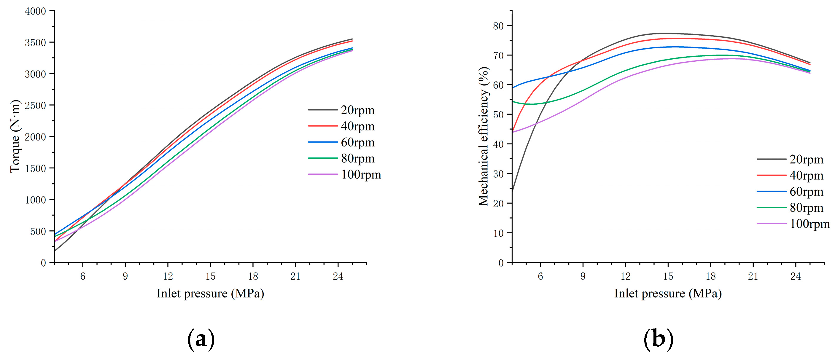
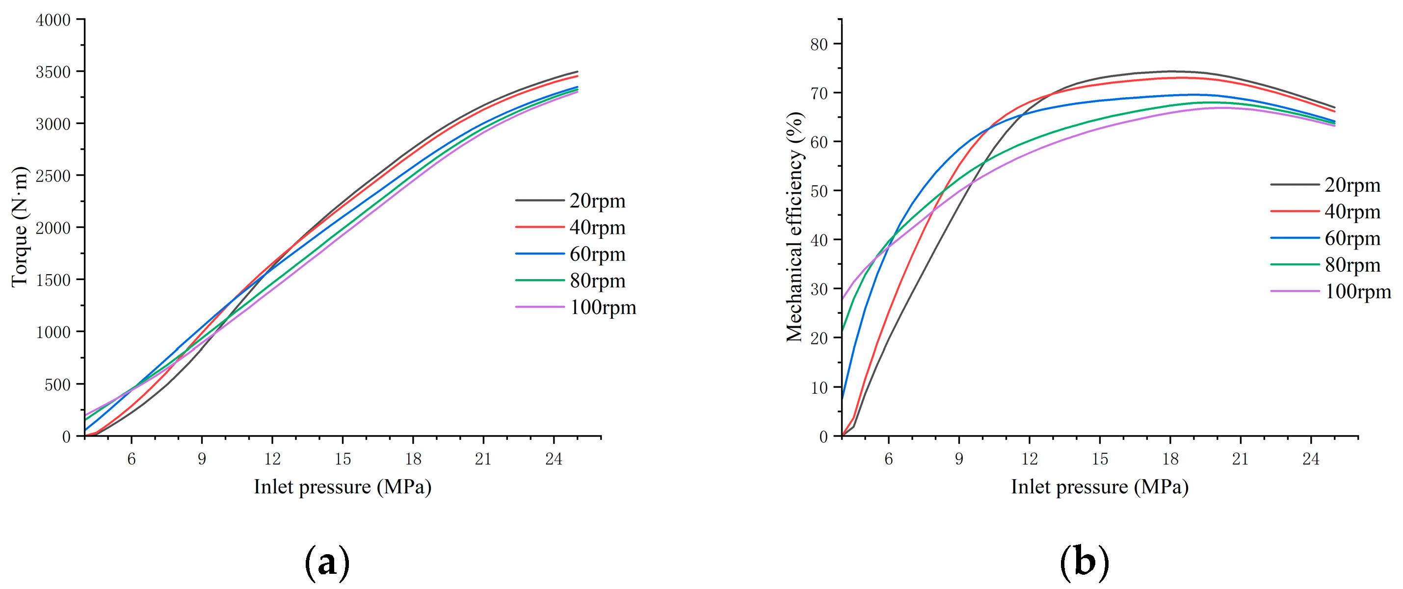
Based on the network’s prediction results, the optimal operating conditions for the motor can be determined. To visually present the variation patterns of the motor’s efficiency and torque under different input conditions, we provide the changes in the motor’s mechanical efficiency and torque with respect to the inlet pressure at different speeds and three different outlet pressures (back pressures) of 0.3 MPa, 0.5 MPa, and 0.7 MPa. As shown in Figure 10, Figure 11 and Figure 12.

From the network prediction results, it is evident that the motor’s output torque has a clear positive correlation with the inlet pressure, while the influence of the speed is minimal. Regarding the mechanical efficiency, several hypotheses can be drawn: 1. When the motor’s inlet pressure changes, the efficiency of motors at higher speeds changes less. 2. For motors operating at low speeds, the outlet pressure should not be too high. 3. The suitable inlet pressure for this motor is in the range of 13–20 MPa.

5. Dynamic Simulation

The torque and efficiency calculation method in the hydraulic system involves measuring the actual output torque (M_S), where the hydraulic fluid works in the hydraulic system, and calculating the mechanical efficiency from the perspective of energy conservation. However, the torque feedback from the dynamic simulation software in this case is the theoretical torque (M_L) caused by the tangential force between the rollers and the stator guide rail under conditions of stable speed and no friction.

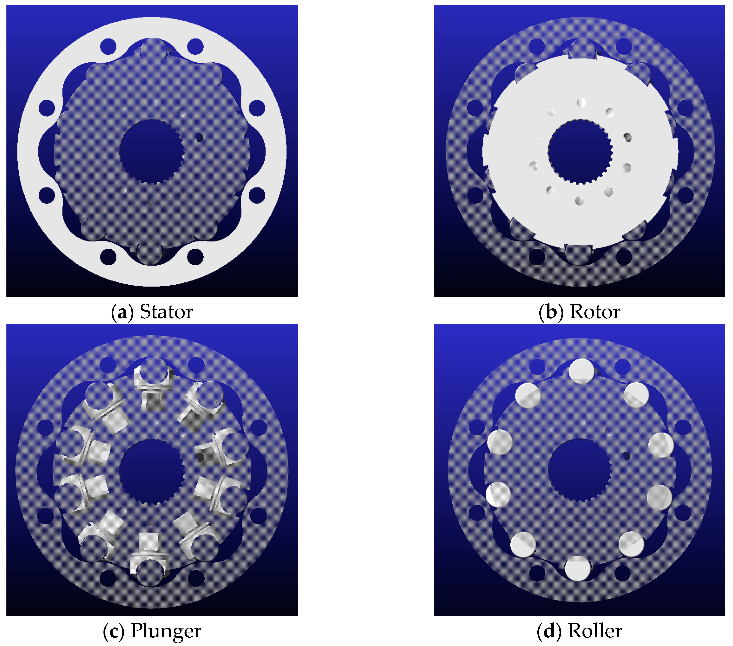
As shown in Figure 13, for the convenience of applying loads to the internal components of the motor and visually displaying the motion of the internal components during motor operation, the dynamic simulation focuses only on the core moving components of the radial piston motor. These components include the stator guide, rotor, piston, and roller.

5.1. Simulation Setup

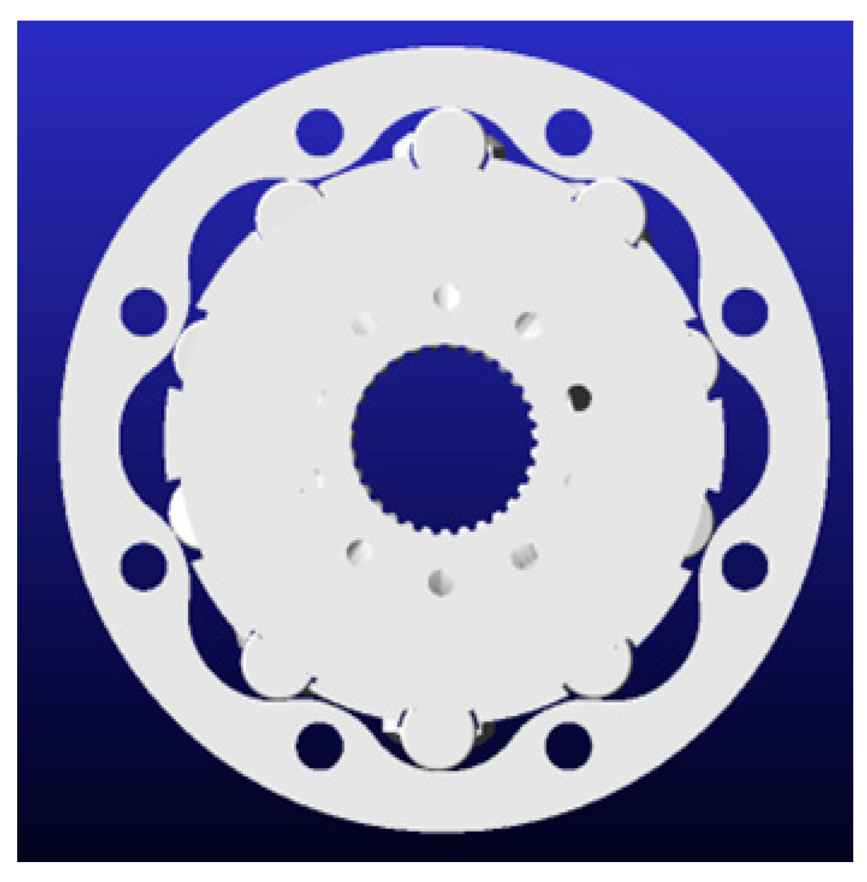
• Importing 3D Models: the model in Adams is shown in Figure 14.

2.

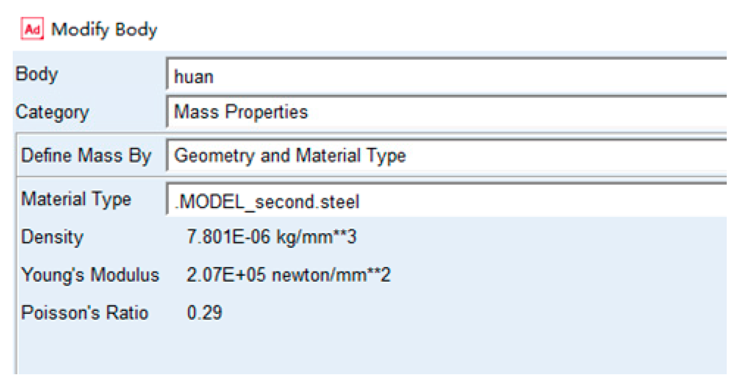
Define Material Properties: the material setting interface in Adams is shown in Figure 15.

Once the material is set, you can view characteristic parameters such as mass, volume, and moments of inertia.

3.

Rename the components to ensure the plunger and roller numbers correspond.

4.

Create Constraint Conditions: the constraints between components are shown in Figure 16.

To apply a fixed constraint between the stator and the ground coordinate system, use a revolute joint between the rotor and the ground coordinate system. Constrain the roller and plunger with a revolute joint and apply a contact constraint between the roller and the stator.

5.

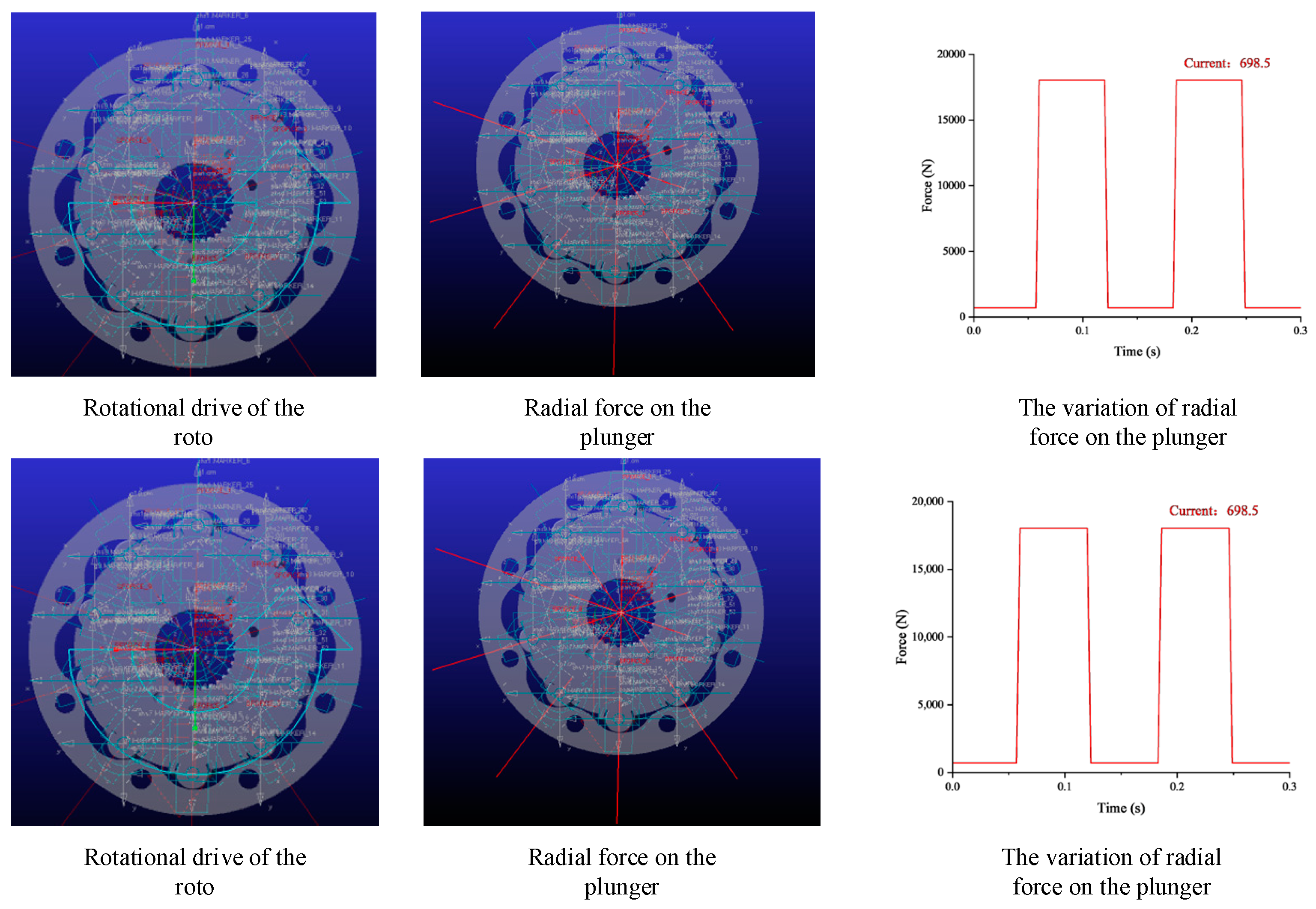
Set up the drivers and apply forces, the changes in forces and the drive are shown in Figure 17.

To apply a rotational drive to the rotor, with its speed determined according to the simulation conditions, set the radial outward fluid pressure on each plunger.

$$F=p{\displaystyle \frac{\pi d^2}{4}}$$

(14)

where F [N] is the force on the plunger, p [pa] is the hydraulic pressure, and d [m] is the effective diameter of the plunger.

To apply hydraulic pressure to the pistons, it is necessary to analyze the angular positions of each piston in the current model. Each piston needs to be individually configured. The pressure changes are instantaneous, transitioning between high pressure (inlet pressure) and low pressure (outlet pressure).

6.

Set up the solver.

7.

Run the simulation.

The simulation model does not include settings for friction between rigid bodies, and the torque obtained after the simulation is theoretical torque. This model can also be used to study the radial motion of pistons, analyze the impact on the stator guide caused by the pistons, and determine the quality of the stator guide’s internal curve form.

5.2. Results of Dynamic Simulation

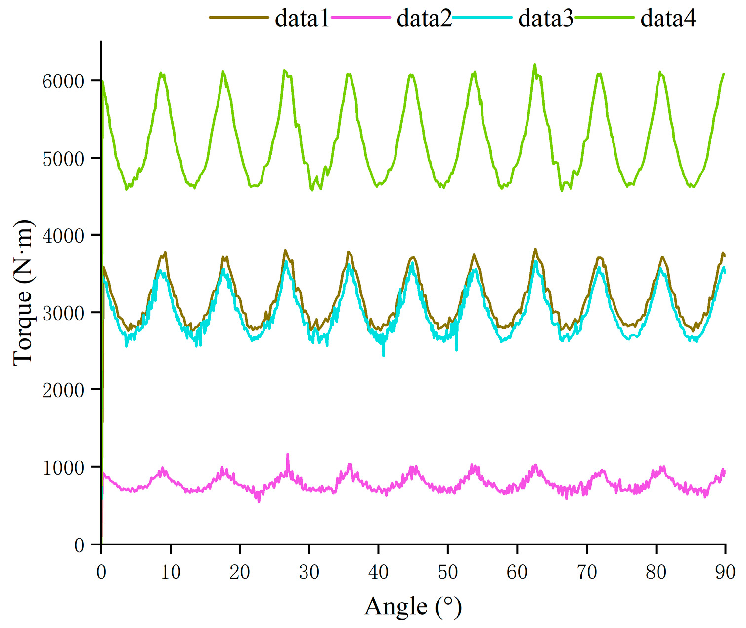
As shown in

Table 5. The Four Selected Data Sets.

Data	Inlet Pressure /MPa	Outlet Pressure /MPa	Speed /rpm	Output Torque /N·m	Mechanical Efficiency/%	Theoretical Torque/N·m
Data 1	15.53	0.6	62	2249.0	70.07	3209.6
Data 2	4	0.3	40	638.7	80.34	795.0
Data 3	14.5	0.3	20	2441	80.02	3050.5
Data 4	25	0.3	20	3593.5	67.71	5307.2

, four data sets were selected to build the dynamic model. Data 1 correspond to the experimental test data 17 from Table 1, used to compare the discrepancy between the simulation and experiment. The other three sets were chosen to verify the accuracy of the network predictions. Data 2 and Data 4 are the peak values from Table 4.

The simulation results of the dynamic model are shown in Figure 18 and

Table 6. Simulation Data Information.

	Maximum Torque /N·m	Minimum Torque /N·m	Average Torque /N·m
Data 1	3819.0	2759.4	3148.5
Data 2	1171.4	540.4	785.4
Data 3	3664.4	2434.0	3001.2
Data 4	6207.3	4568.9	5224.2

. The torque simulation results exhibit pulsations caused by the inner curve of the stator ring. Improving the shape of the inner curve of the stator ring can reduce torque pulsations to some extent. The simulation terminates after the rotor rotates 90°, during which the plungers complete two radial expansion and contraction cycles.

From Figure 18, it can be seen that when the inlet pressure of the hydraulic motor is high, the torque pulsations are significant. Under low inlet pressure conditions, the torque remains relatively stable.

The discrepancies between the theoretical torque values in Table 5 and the average torque values from the simulation results in Table 6 are 1.9%, 1.2%, 1.6%, and 1.6%, respectively.

6. Conclusions

Through the analysis of experimental data on the radial piston motor, suitable operating conditions for the motor can be determined. Conducting efficiency measurement experiments, employing linear regression and neural networks to predict experimental data, and constructing a dynamic model, the following conclusions can be drawn:

• The neural network fits the torque information from the experimental data very well, making it suitable for predicting the torque under different operating conditions of the motor.
• The torque results from the physical experiments are consistent with those from the dynamic simulation model, indicating that using a dynamic simulation to obtain the theoretical torque of the radial piston motor is feasible. This method can provide a reference for the actual operation of the motor.
• According to the predictions of the neural network, the motor’s mechanical efficiency is stable under low-speed conditions; however, under high-speed conditions, the inlet pressure needs to be appropriately adjusted to achieve good mechanical efficiency.

References

1. Strmčnik, E.; Majdič, F.; Kalin, M. Water-lubricated behaviour of AISI 440C stainless steel and a DLC coating for an orbital hydraulic motor application. Tribol. Int. 2019, 131, 128–136. [Google Scholar] [CrossRef]
2. Pettersson, U.; Jacobson, S. Textured surfaces for improved lubrication at high pressure and low sliding speed of roller/piston in hydraulic motors. Tribol. Int. 2007, 40, 355–359. [Google Scholar] [CrossRef]
3. Zhang, D.; Li, Z.; Wang, L.; Kong, L.; Gao, F.; Wang, Q. Study on tribological properties of boronized and textured composite surface and its application on camshaft connecting-rod type hydraulic motor. Wear 2021, 482, 203964. [Google Scholar] [CrossRef]
4. Qiu, B.; Zhao, J.; Man, J. Comparative study of materials for friction pairs in a new high water-based hydraulic motor with low speed and high pressure. Ind. Lubr. Tribol. 2019, 71, 164–172. [Google Scholar] [CrossRef]
5. Lyu, F.; Zhang, J.; Zhao, S.; Li, K.; Xu, B.; Huang, W.; Xu, H.; Huang, X. Coupled evolution of piston asperity and cylinder bore contour of piston/cylinder pair in axial piston pump. Chin. J. Aeronaut. 2023, 36, 395–407. [Google Scholar] [CrossRef]
6. Ceschini, L.; Marconi, A.; Martini, C.; Morri, A. Tribological behavior of components for radial piston hydraulic motors: Bench tests, failure analysis and laboratory dry sliding tests. Wear 2013, 305, 238–247. [Google Scholar] [CrossRef]
7. Wang, Z.; Wu, S.; Gao, D.; Wang, S. Distribution Performance Analysis and Experimental Research on the Port Plate Pairs of Low Speed High Torque Seawater Hydraulic Motor. Chin. J. Mech. Eng. 2019, 32, 108. [Google Scholar] [CrossRef]
8. Patrosz, P. Influence of Properties of Hydraulic Fluid on Pressure Peaks in Axial Piston Pumps’ Chambers. Energies 2021, 14, 3764. [Google Scholar] [CrossRef]
9. Quan, L.; Gao, H.; Guo, C.; Che, S. Assessment of the Dynamics Flow Field of Port Plate Pair of an Axial Piston Pump. Processes 2020, 8, 86. [Google Scholar] [CrossRef]
10. Sliwinski, P.; Patrosz, P. Methods of Determining Pressure Drop in Internal Channels of a Hydraulic Motor. Energies 2021, 14, 5669. [Google Scholar] [CrossRef]
11. Manne, V.H.B.; Vacca, A.; Merrill, K. A numerical method for evaluating the torque efficiency of hydraulic orbit motors considering deformation effects and frictional losses. Mech. Syst. Signal Process. 2021, 146, 107051. [Google Scholar] [CrossRef]
12. Nie, Y.; Niu, Y.; Xing, K.; Jin, X. Hydraulic motor constant low speed characteristics measurement study. J. Phys. Conf. Ser. 2005, 2005, 012237. [Google Scholar] [CrossRef]
13. Liu, Y.; Deng, Y.; Fang, M.; Li, D.; Wu, D. Research on the torque characteristics of a seawater hydraulic axial piston motor in deep-sea environment. Ocean Eng. 2017, 146, 411–423. [Google Scholar] [CrossRef]
14. Sliwinski, P. Determination of the Theoretical and Actual Working Volume of a Hydraulic Motor. Energies 2020, 13, 5933. [Google Scholar] [CrossRef]
15. Liu, G.; Zhou, Z.; Qian, X.; Wu, X.; Pang, W. Multidisciplinary Design Optimization of a Swash-Plate Axial Piston Pump. Appl. Sci. 2016, 6, 399. [Google Scholar] [CrossRef]
16. Li, R.; Liu, J.; Ding, X.; Liu, Q. Study on the Influence of Flow Distribution Structure of Piston Pump on the Output of Pulsation Pump. Processes 2022, 10, 1077. [Google Scholar] [CrossRef]
17. Ying, P.; Tang, H.; Chen, L.; Ren, Y.; Kumar, A. Dynamic modeling and vibration characteristics of multibody system in axial piston pump. Alex. Eng. J. 2023, 62, 523–540. [Google Scholar] [CrossRef]
18. Li, R.; Liu, Q.; Cheng, Y.; Liu, J.; Sun, Q.; Zhang, Y.; Chi, Y. Analysis of the Influence of Structure and Parameters of Axial Piston Pump on Flow Pulsation. Processes 2022, 10, 2138. [Google Scholar] [CrossRef]
19. Suo, X.; Jiang, Y.; Wang, W. Hydraulic axial plunger pump: Gaseous and vaporous cavitation characteristics and optimization method. Eng. Appl. Comput. Fluid Mech. 2021, 15, 712–726. [Google Scholar] [CrossRef]
20. Zhang, C.; Tan, H.; Fang, Y.; Zhang, X.; Yang, Y.; Duan, Y.; Han, M.; Cui, S.; Xu, B.; Zhang, J. Deformation pre-compensated optimization design of cam ring for low pulsation hydraulic motors. J. Zhejiang Univ.-SCIENCE A 2023, 24, 130–145. [Google Scholar] [CrossRef]
21. Shen, H.; Zhou, Z.; Guan, D.; Liu, Z.; Jing, L.; Zhang, C. Dynamic Contact Analysis of the Piston and Slipper Pair in Axial Piston Pump. Coatings 2020, 10, 1217. [Google Scholar] [CrossRef]
22. Zhang, J.; Xia, S.; Ye, S.; Xu, B.; Zhu, S.; Xiang, J.; Tang, H. Sound quality evaluation and prediction for the emitted noise of axial piston pumps. Appl. Acoust. 2019, 145, 27–40. [Google Scholar] [CrossRef]
23. Ramchandran, G.; Agarwal, P.; Vacca, A.; Kim, K.S.; Kim, T. Modeling of radial piston machines considering elastohydro dynamic effects in both cam–piston and piston–cylinder lubricating interfaces. Meccanica 2018, 53, 2833–2860. [Google Scholar] [CrossRef]
24. Nilsson, D.; Prakash, B. Investigation into the seizure of hydraulic motors. Tribol. Int. 2010, 43, 92–99. [Google Scholar] [CrossRef]
25. Cheng, L.; Chen, X.; Wei, G. Cylinder Fatigue Design of Low-Speed, High-Torque Radial Piston Motor. Coatings 2022, 12, 1192. [Google Scholar] [CrossRef]
Figure 1. Radial Piston Motor Structure Diagram.
Machines 12 00491 g001
Figure 2. Contact Force between Roller and Stator.
Machines 12 00491 g002
Figure 3. Schematic diagram of hydraulic system: 1 Filter; 2 Hydraulic pump; 3 Motor; 4, 14 Relief valve; 5, 8, 13 Pressure gauge; 6 Throttle valve; 7, 15, 16 Flow meter; 9 Radial plunger motor; 10 Coupling; 11 Torque sensor; 12 Load motor.
Machines 12 00491 g003
Figure 4. Radial plunger motor test platform.
Machines 12 00491 g004
Figure 5. Scatterplot matrix.
Machines 12 00491 g005
Figure 6. This is a figure. Schemes follow the same formatting.
Machines 12 00491 g006
Figure 7. Neural Network Flowchart.
Machines 12 00491 g007
Figure 8. Neural Network Architecture.
Machines 12 00491 g008
Figure 9. The fitting status of the output torque neural network: (a) represents the fitting results for the 23 training set samples; (b) represents the fitting results for the 7 testing set samples.
Machines 12 00491 g009
Figure 10. Outlet pressure: 0.3 MPa. (a) Torque Variation Diagram; (b) Mechanical Efficiency Variation Diagram.
Machines 12 00491 g010
Figure 11. Outlet pressure: 0.5 MPa. (a) Torque Variation Diagram; (b) Mechanical Efficiency Variation Diagram.
Machines 12 00491 g011
Figure 12. Outlet pressure: 0.7 MPa. (a) Torque Variation Diagram; (b) Mechanical Efficiency Variation Diagram.
Machines 12 00491 g012
Figure 13. The structure of the dynamic model.
Machines 12 00491 g013
Figure 14. Three-Dimensional Models in Adams.
Machines 12 00491 g014
Figure 15. Material selection: steel.
Machines 12 00491 g015
Figure 16. Constraint conditions.
Machines 12 00491 g016
Figure 17. Drive and force in ADAMS.
Machines 12 00491 g017
Figure 18. Simulated Torque Result.
Machines 12 00491 g018