Human Reliability Assessment of Space Teleoperation Based on ISM-BN

Abstract

Space teleoperation systems, as complex giant systems, feature performance-influencing factors that are interrelated. Accurately describing the dependence between these factors is crucial for constructing a human factor reliability assessment (HRA) model. Moreover, data scarcity has consistently been a challenge in space HRA. There are primarily two types of data in this domain: expert judgment data and empirical data (simulation data, actual reports), each with complementary effects. The expert judgment data, although subjective, are readily accessible, while empirical data provide robust objectivity but are difficult to obtain. Addressing these challenges, this paper constructs an HRA model for space teleoperation that combines Interpretive Structural Modeling (ISM) with a two-stage Bayesian update method. This model reflects the dependencies between factors and accommodates multisource data (expert judgment and experimental data). With more empirical data, the model can be continuously updated and refined to yield increasingly accurate evaluations of human error probability (HEP). The validity of the model was verified through the analysis of 52 space incidents using the N-K model. The study provides a methodological foundation for HRA in other space missions.

1. Introduction

Human reliability assessment (HRA) is an integral part of probabilistic safety assessment that focuses on the impact of human error on system safety. HRA often quantitatively evaluates the probability of human error using empirical data. In the study of the mechanism of human error, the evaluation and prediction of human behavior are achieved through victory and other indicators [1,2,3]. HRA pays more attention to the macroscopic connection among factors and their effects on human error.

The causation of space accidents or incidents is often attributed to the synergistic effects of multiple risk factors [4]. However, the lack of reliable standards for establishing the interrelations (dependencies) among these factors may render current human reliability assessment (HRA) models flawed [5]. If the dependencies of these factors are not reasonably considered, the resultant risk assessments may be misleading [6]. Traditional HRA methods (such as CREAM [7], SPAR-H [8], and IDAC [9]) have considered the dependencies of factors to varying extents, yet these methods have not quantitatively described the dependencies. To address the shortcomings (such as CREAM [7], SPAR-H [8], and IDAC [9]), the dependencies of factors are considered to varying extents, yet these methods have not quantitatively described the dependencies. To address the shortcomings of these traditional approaches, studies have integrated Fuzzy Inference Rules [10], Analytic Network Process [11] (ANP), and Bayesian networks [12] (BNs) to enhance the precise quantitative expression of the dependencies. Furthermore, statistical approaches (e.g., structural equation modeling [10], logistic regression [13]) have also been applied to investigate the combined effects of factors on HEP. Efforts have been made to extract dependencies from a multitude of event reports. However, this requires a high quantity and quality of accident reports, posing a significant challenge for the aerospace field, where data are inherently scarce.

BNs offer significant advantages in inferring events with uncertain dependencies and have been widely applied in HRA [14]. The uncertainty of Bayesian networks mainly comes from the determination of topology and conditional probability [15].

On the one hand, the topology of the BNs is frequently judged based on experience [16,17], which lacks traceability. The establishment of the topology expresses the dependency between the influencing factors to some extent. As mentioned above, several methods have been proposed to quantify the dependency between factors. The fuzzy rule and DEMATEL method express the relationship between any two factors through subjective expert judgment. In data-rich domains, structure learning can be used to construct structures [18]. However, in the aerospace field, it is difficult to find adequate data-support structures for learning. Compared to these methods, Interpretive Structural Modeling [19,20] (ISM) reduces the reliance on large quantities of survey data, making it more suitable for fields such as space fields where data are scarce. In addition, ISM intuitively expresses the relationship between multiple factors using a hierarchical structure. Although this hierarchy structure is not equal to the topological structure of the BN, combining ISM with BN can reduce uncertainty [21].

On the other hand, a major impediment to the development of HRA models is the scarcity of accessible, valid observational data or historical records related to space teleoperation incidents [22]. This undoubtedly increases the uncertainty of the constructed model. In data-rich domains such as medical diagnostics and finance, these distributions can be determined through parameter learning [23]. However, the scarcity of data in the space sector often results in insufficient data for learning BN parameters. Sources of human reliability data in the space field primarily include empirical data (such as on-orbit experiments, incident/accident analysis reports, training data/simulator trials, laboratory experiments) and expert judgment data [24]. On-orbit and training data are of high precision but are often difficult to access due to confidentiality regulations in space missions. In contrast, the availability of experimental data is significantly greater. Experiments typically control extraneous variables to study the dependence between independent and dependent variables, thus providing the most accessible empirical data for the dependence between factors and HEP. However, experimental data may lack authenticity in terms of the experimental group and environment and fail to observe the dependencies between numerous factors and HEP simultaneously [25]. Expert judgment compensates for these deficiencies, as domain experts are often involved throughout the entire process. Although expert judgment data are subjective and uncertain [26], they may yield information not contained within empirical data. Thus, there is an urgent need for an assessment method that can accommodate multisource data to garner more information for HRA in space teleoperation.

Consequently, this paper integrates ISM with BN to construct an HRA model for space teleoperation. ISM is utilized to build the topological structure of dependencies between factors, while BN facilitates a two-stage update of expert and experimental data, offering the potential for continuous model updates as more data become available. The structure of this paper is organized as follows: Section 2 introduces the methods employed in this study; Section 3 presents the results of the model construction; Section 4 validates the model through event analysis using the N-K model; and Section 5 concludes the paper.

2. Materials and Methods

The method of this study is illustrated in Figure 1. First, the qualitative structure between factors was constructed through ISM based on results from [27]. These dependencies are then mapped onto a BN within a tiered network model constructed for space teleoperation safety analysis, facilitating the transformation of a conditional probability distribution.

Subsequently, the Bayesian update method of aggregating expert opinions [28] is used to update the conditional probabilities in BNs in a stage-wise manner using domain expert judgment information. Specifically, the β distribution [8,29] models the uncertainty of HEP in this paper, and the conditional probability of the extreme state of a node is estimated by domain experts. The conditional probabilities of all BN nodes are obtained using the function interpolation method, thus acquiring the conditional probability parameters of BNs. The core of this approach is the assumption that HEP parameters follow a certain distribution, which is updated to a posteriori distribution by collecting evidence (expert judgment or experimental data) to achieve a more accurate representation of HEP.

The posterior distribution obtained from the first-stage expert judgment update serves as the prior distribution for the second-stage Bayesian update. The experimental data in this study are used to update the conditional probability in BNs [30]. This two-stage updated BN model can realize the quantitative evaluation of task performance and fill the gap in research on the evaluation of robotic arm-assisted extravehicular operators due to error. The Bayesian update method described in this chapter can be used to gradually update the BN parameters when more empirical data become available in the future, thereby obtaining more accurate evaluation results and providing a reference for improving the safety management system of aerospace teleoperation.

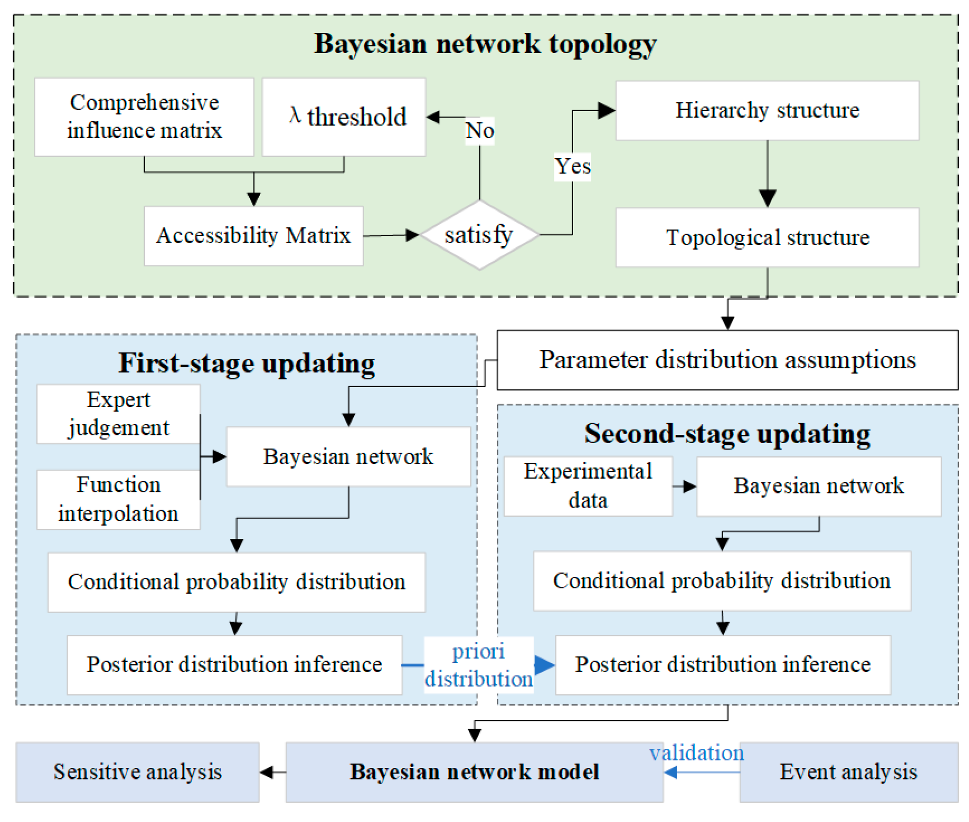
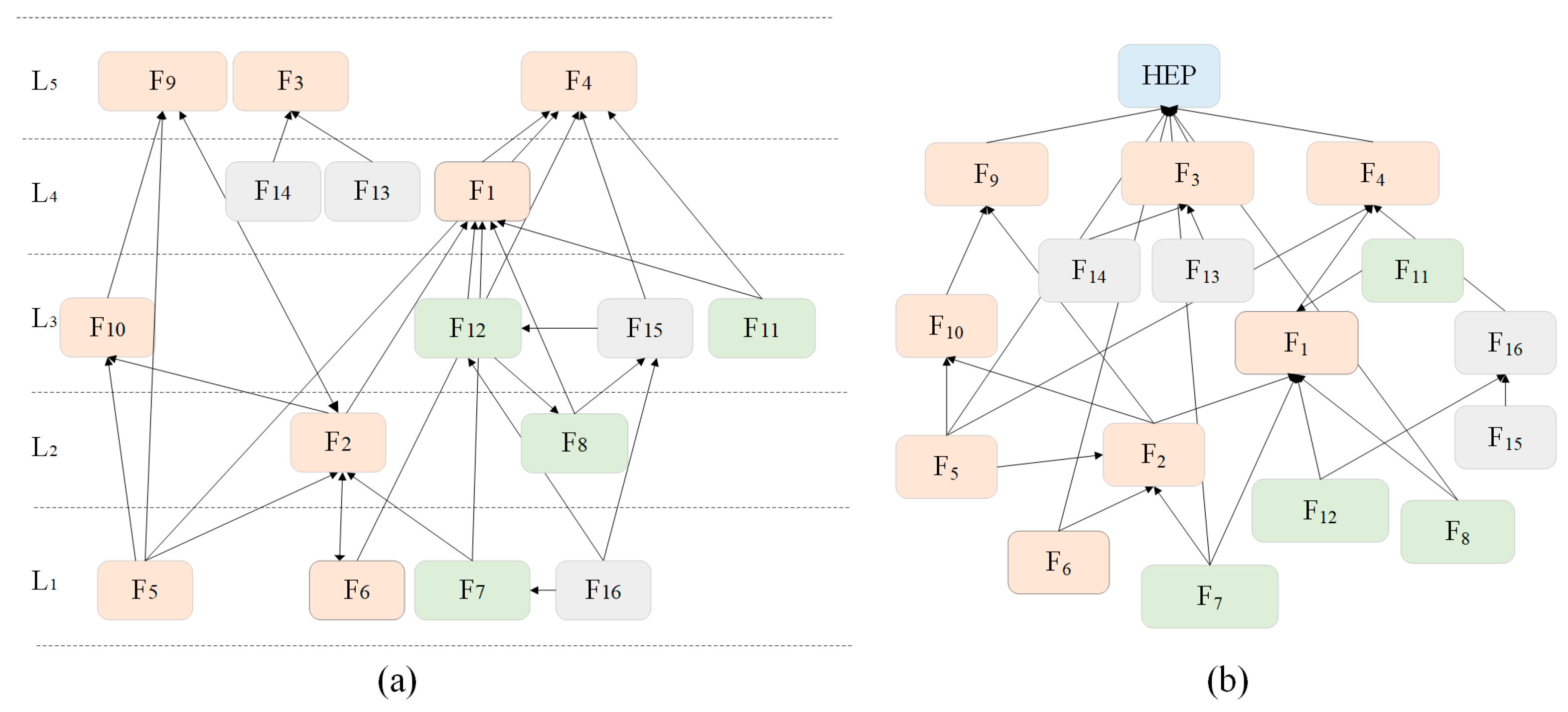
2.1. Interpretive Structural Modeling

Interpretive structural modeling (ISM) based on the Decision-Making Trial and Evaluation Laboratory [31] (DEMATEL) facilitates the identification of hierarchical structures among influencing factors, simplifying the analysis of interrelations and hierarchy of risk factors [32]. This method primarily uses a reachability matrix to represent interactions and hierarchical relations among factors.

For a set with n factors, there exists a total relation matrix $\mathit{T}={\left[t_{ij}\right]}_{n\times n}$, where $t_{ij}$ represents the influence of factor $i$ on the factor $j$. For space teleoperation, T can be derived from [27]. However, T does not consider the self-impact of the involved factors. To address this, the identity matrix I, which represents the self-impact of the factors, is introduced to obtain the overall-influence matrix $\mathit{H}={\left[h_{ij}\right]}_{n\times n}$.

$$\mathit{H}=\mathit{I}+\mathit{T}$$

(1)

The objective of ISM is to hierarchically divide factors using a reachability matrix. Initially, determination of the threshold λ of the dependence is necessary to facilitate the division of the system hierarchy. Typically, λ can be set by experts or decision-makers based on real problems. To reduce the subjective effect of λ directly given by experts, this study utilizes Equation (2) to calculate λ [33].

$$\lambda =\beta +\gamma$$

(2)

where β is the mean of the comprehensive impact matrix $\mathit{T}$, and γ is the standard deviation of the comprehensive impact matrix $\mathit{T}$. The influence matrix (K) is obtained by the Equation (3), $\mathit{K}={\left[k_{ij}\right]}_{n\times n}$.

$$k_{ij}=\left\{\begin{array}{c}0,h_{ij}<\lambda \\ 1,h_{ij}\ge \lambda \end{array},i,j=1,2,\dots ,n\right.$$

(3)

Based on K, the reachable set (R) and antecedent set (A) of the factors in the involved system can be defined. $R$ represents all factors in K where the corresponding row values are 1, and $A$ represents the row set where the corresponding column value is 1. When both these sets of factors satisfy Equation (4), the factor is classified into the first layer, and its rows and columns are removed from K to generate a new reachability matrix. This layer-by-layer analysis yields a clear hierarchy of factors for space teleoperation.

$$\mathit{R}\left(F_i\right)\mathit{A}\left(F_i\right)=\mathit{R}\left(F_i\right)$$

(4)

2.2. Probabilistic Interpretation of HRA

The HEP of an HFE is denoted as $p$, and the mean value of the HEP is expressed as $\theta$. A specific combination of factors is denoted as $\mathit{F}$, which defines the combination of specific factors and their levels. The prediction results of HRA usually represent the mean HEP under $\mathit{F}$. Thus, the prediction process of HRA can be expressed as a mapping from $\mathit{F}$ to $\theta$:

$$\mathit{F}\to \theta$$

(5)

It is assumed that $p$ follows a lognormal distribution in THERP and ASEP [34]. However, the lognormal distribution can yield results greater than 1. Therefore, SPAR-H [8] used β distribution to describe $p$. The β distribution is a two-parameter ($\alpha$ and $\beta$) distribution [24]. By adjusting these parameters, the distribution can be tailored to various data distributions (such as U-shaped, normal, uniform, or exponential), thereby enhancing the model’s fitting capability. Assume that $p$ follows a β distribution with parameters α and $\beta$. According to [35], α = 0.5 and β can be obtained from

$$\beta =\frac{\left[\alpha \left(1-\theta \right)\right]}{\theta }$$

(6)

According to human information processing [36], we divide the types of human error into perceptual, decision-making, and execution errors. Their probabilities are denoted by $p^{\mathrm{p}}$, $p^{\mathrm{d}}$, and $p^{\mathrm{e}}$, respectively. The total HEP of HFE can then be expressed as follows [37]:

$$p=1-\left(1-p^{\mathrm{p}}\right)\left(1-p^{\mathrm{d}}\right)\left(1-p^{\mathrm{e}}\right)$$

(7)

2.3. First-Phase Update Based on Expert Judgement Data

HEP (variable p) is a continuously distributed random variable located in the interval [0,1], which is discretized to facilitate engineering application. The [0,1] interval was discretized into five intervals, and a reference value $x_i$ was selected for each interval. The maximum reference value of HEP was $x_5$ defined as 0.5, considering the low probability of space accidents. Other $x_i$ values were obtained according to the gradient of 1/5 times. The boundary value of each interval is the geometric mean of $x_i$ in the two consecutive intervals. In the following, $p$ and $\theta$ can only fall into one of these five intervals. The probability that the variable HEP ($p$) falls in each interval is obtained by integrating the β distribution over the corresponding probability interval (

Table 1. HEP discretization.

Interval	Label	Reference Value	Probabilistic Boundary
1	Very low	$x_1=0.0008$	$\left[a_1,b_1\right)=\left[0, 0.00179\right)$
2	Low	$x_2=0.004$	$\left[a_2,b_2\right)=\left[0.00179,0.0089\right)$
3	Medium	$x_3=0.02$	$\left[a_3,b_3\right)=\left[0.0089,0.045\right)$
4	High	$x_4=0.1$	$\left[a_4,b_4\right)=\left[0.045,0.22\right)$
5	Very high	$x_5=0.5$	$\left[a_5,b_5\right)=\left[0.22,1\right]$

).

It is assumed that there is a prior distribution (${\pi }^0$) of $\theta$ before expert judgment. By judging $\theta$ values through experts, a statistical evidence set ${\mathit{E}}^1=\left\{x{ }_{i_1^{\ast }},x_{i_2^{\ast }},\dots ,x_{i_h^{\ast }}\right\}$ can be obtained, where $x_{i_{h }^{\ast }}$ indicates that expert $h$ thinks $\theta$ is in interval $i_{h }^{\ast }$. To reduce the workload and uncertainty of expert judgment, experts only need to judge the factors located at the extreme level. Other combinations of factors located at the intermediate level can be obtained by linear interpolation.

From the Bayesian theorem, the posterior distribution of θ can be updated as follows:

$${\pi }^1\left(\theta \right)=Pr\left(\theta |{\mathit{E}}^1\right)=\frac{L^1({\mathit{E}}^1|\theta ){\pi }^0\left(\theta \right)}{{\sum }_{\theta }(L^1({\mathit{E}}^1|\theta ){\pi }^0\left(\theta \right))}$$

(8)

where ${\pi }^0\left(\theta \right)$ is the prior distribution of θ, which is assumed to follow a uniform distribution, ${\pi }^0\left(\theta =x_1\right)=\cdots ={\pi }^0\left(\theta =x_5\right)=0.2$. $\sum _{\theta }(L^1({\mathit{E}}^1|\theta ){\pi }^0\left(\theta \right))$ normalize the ${\pi }^1\left(\theta \right)$ as a probability distribution. $L^1({\mathit{E}}^1|\theta )$ is the likelihood term, which indicates the probability of observing ${\mathit{E}}^1$ when $\theta$ is known. An expert’s judgment corresponds to a specific realization of $p$, denoted as $p^{\ast }$. It is assumed that each expert completes judgment independently. That is, when $\theta$ is known, the judgment result of each expert is conditionally independent. Therefore, according to the condition-independent definition, $L^1\left({\mathit{E}}^1|\theta \right)$ can be calculated using Equation (9) as follows:

$$L^1\left({\mathit{E}}^1|\theta \right)={\prod }_{h=1}^H{L}_h^1\left(p_h^{\ast }=x_{i_{h }^{\ast }}|\theta \right)$$

(9)

Among them, $L_h^1\left(p_h^{\ast }=x_{i_{h }^{\ast }}|\theta \right)$ is the likelihood term of each expert. Denote the judgement of expert $h$ as $p_h^{\ast }$ when $\theta$ is known. The probability of $p_h^{\ast }=x_{i_{h }^{\ast }}$ is $L_h^1$. H is the total number of experts. Depending on the independent nature of the condition, $L_h^1\left(p_h^{\ast }=x_{i_{h }^{\ast }}|\theta \right)$ can be calculated by Equation (10).

$$L_h^1\left(p_h^{\ast }=x_{i_{h }^{\ast }}|\theta =x_j\right)={\sum }_{p^{\ast }}\mathit{Pr}\left(p_h^{\ast }=x_{i_{h }^{\ast }}|p^{\ast }\right)\mathit{Pr}\left(p^{\ast }|\theta =x_j\right)={\sum }_{k=1}^5{g}_{i_{h }^{\ast }k}{f}_{kj}$$

(10)

where $f_{kj}$ represents the probability that the $p^{\ast }$ is in the $k$th interval when $\theta$ is in the $j$th scale. It can be calculated from the probability density of the β distribution.

$$f_{kj}=\mathit{Pr}\left(p^{\ast }=x_k|\theta =x_j\right)dx={{\displaystyle \int }}_{a_j}^{b_j}\frac{1}{\mathrm{B}\left(\alpha ,\beta \right)}{x}^{\alpha -1}{\left(1-x\right)}^{\beta -1}x$$

(11)

where $betapdf\left(x,\alpha ,\beta \right)$ represents the probability density function of the β distribution with parameters of $\alpha ,\beta$. $a_j$,$b_j$ denotes the interval range of the $j$th scale after discretization. Therefore, $f_{kj}$ represents the inherent variability of HEP. $g_{i_h^{\ast }k}$ is the probability that $p_h^{\ast }$ fall in the $i_h^{\ast }$ interval when $p^{\ast }$ is in the $k$th scale. Therefore, $g_{i_h^{\ast }k}$ represents confidence in the expert’s judgment of HEP results. For the convenience of calculation, we assume that $g_{i_h^{\ast }k}$=$f_{i_h^{\ast }k}$.

Combined with all the formulas in this section, the above posterior distribution inference for $\theta$ can be realized. Note that in BNs, what is ultimately obtained is a conditional probability regarding $p$. Therefore, the posterior distribution ${\tau }^1\left(p\right)$ of HEP needs to be calculated using the full probability formula, as shown in Equation (12).

$${\tau }^1\left(p=x_k\right)={\sum }_{\theta }[Pr(p=x_k|\theta ){\pi }^1\left(\theta \right)]={\sum }_j{f}_{kj}{\pi }^1\left(\theta =x_j\right)$$

(12)

2.4. Second-Phase Update Based on Experimental Data

After updating the distribution of parameters with evidence judged by experts in Section 2.3, the conditional probabilities required for BNs are determined. The preliminary parameterization and construction of the model are realized using prior and conditional probabilities. However, because of the inevitable subjectivity of expert judgment, we can update the constructed model using empirical data such as experiments to improve accuracy.

The total HEP of a particular operator performing that task under a particular condition is denoted as $p_{\mathrm{o}}$. Assume that $p_{\mathrm{o}}$ also obeys a β distribution with parameters α and β, which can be determined by Equation (13).

$$\beta =\left[\alpha \left(1-p^{\ast }\right)\right]/p^{\ast }$$

(13)

where $p^{\ast }$ denotes a single realisation (realisation) of the variable $p$. $p^{\ast }$ responds to the probability of HFE when that specific task is performed by an average person under that combination (without considering exactly who performs it). The uncertainty in $p^{\ast }$ arises only from within-categories variability. The distribution of $p_{\mathrm{o}}$ is determined by its distributional parameters (α and β) (α and β are calculated from $p^{\ast }$ according to Equation (10). The uncertainty in $p_{\mathrm{o}}$ arises from crew variability.

Then, the update can be performed using the Bayesian theorem as follows:

$${\pi }^2\left(\theta \right)=Pr\left(\theta |{\mathit{E}}^2\right)=\frac{L^2({\mathit{E}}^2|\theta ){\pi }^1\left(\theta \right)}{{\sum }_{\theta }(L^2({\mathit{E}}^2|\theta ){\pi }^1\left(\theta \right))}$$

(14)

where ${\pi }^2$ is the posterior distribution of $\theta$ after updating using the experiment data. ${\pi }^1$ not only represents the posterior distribution of $\theta$ after aggregation of expert opinions but it also serves as the prior distribution for the second stage updating. $L^2({\mathit{E}}^2|\theta )$ represents the likelihood term, which denotes the probability of observing the evidence ${\mathit{E}}^2$ when $\theta$ is known. ${\mathit{E}}^2=\left\{{\mathit{E}}_1^2,{\mathit{E}}_1^2,\dots ,{\mathit{E}}_S^2\right\}=\left\{\left(T_1,T\right),\left(T_2,T\right),\dots ,\left(T_S,T\right)\right\}$ represents the observed experiment result that subject $s$ made $T_s$ times failures in $T$ times trails. For example, one subject conducted two experiments, but only one of them was incorrect. It is expressed as ${\mathit{E}}_1^2=\left(1,2\right)$. $\sum _{\theta }(L^2({\mathit{E}}^2|\theta ){\pi }^1\left(\theta \right))$ normalize ${\pi }^2\left(\theta \right)$ to a probability distribution.

$$L^2\left({\mathit{E}}^2|\theta \right)={\sum }_{p^{\ast }}\mathit{Pr}\left({\mathit{E}}^2|p^{\ast }\right)\mathit{Pr}\left(p^{\ast }|\theta \right)$$

(15)

where $\mathit{Pr}\left({\mathit{E}}_s^2|p^{\ast }\right)$ denotes the probability of observing evidence ${\mathit{E}}_s^2$ when the $p^{\ast }$ is known. $\mathit{Pr}\left(p^{\ast }|\theta \right)$ denotes the probability that the HEP for that task is $p^{\ast }$ when the mean HEP ($\theta$) is known. Since each subject completed the experiment independently, the subjects’ results are conditionally independent. Then Equation (15) can be further written as

$$L^2\left({\mathit{E}}^2|\theta \right)={\sum }_{p^{\ast }}\{\mathit{Pr}\left(p^{\ast }|\theta \right){\prod }_{s=1}^S[{\sum }_{p_o^{\ast }}\mathit{Pr}\left(p_o^{\ast }|p^{\ast }\right)Bin\left(T_s,T,p_o^{\ast }\right)]\}$$

(16)

where $\sum _{p_o^{\ast }}\mathit{Pr}\left(p_{\mathrm{o}}|p^{\ast }\right)Bin\left(T_s,T,p_o^{\ast }\right)$ is expanded according to the full probability equation. $\mathit{Pr}\left(p_{\mathrm{o}}|p^{\ast }\right)$ denotes that the probability of failure of the subject to perform the task is $p_o^{\ast }$ when $p^{\ast }$ of the task is known. $Bin\left(T_s,T,p_o^{\ast }\right)$ denotes the probability of $T_s$ times failures occurring in $T$ times independently repeated experiments when $p_o^{\ast }$ is known.

Combined with Equations (14)–(16), the posterior distribution of $\theta$ can be updated by experiment data. The posterior distribution of HEP, denoted as ${\tau }^2\left(p\right)$, can be calculated by Equation (17).

$${\tau }^2\left(p=x_k\right)={\sum }_{\theta }[Pr(p=x_k|\theta ){\pi }^2\left(\theta \right)]={\sum }_j{f}_{kj}{\pi }^2\left(\theta =x_j\right)$$

(17)

3. Results

The definition of F₁–F₁₆ is shown in [27]. Among them, red represents the human factor, green represents the machine factor, and gray represents the situational factor. The hierarchical structure of influencing factors was determined based on ISM Figure 2a. The dependence between factors is complex. There are circular connections between some factors in Figure 2b, which are not allowed in BN. Therefore, adjustments were made based on rules [21] to remove redundant links and make them more suitable for BN representation. These rules are as follows: (1) retain only links with direct dependence; (2) for factors with relative independence, the decision to remain pointing or directed links is based on whether they are causal factors; (3) eliminate any circular relationships to satisfy the acyclic structure of BN; (4) add top-level failure modes to the original hierarchical structure of influencing factors.

Since the number of conditional probabilities required for BN inference grows exponentially with the number and level of nodes [38]. To control the workload involved in quantifying the parameters of the BN, the levels of the above factors are set at 2–3 levels. In this study, a 35-person domain expert judgment was organized. Each expert should determine which of the above reference values was the possible value of perceived error ($p^{\mathrm{p}}$), decision-making error ($p^{\mathrm{d}}$), and execution error ($p^{\mathrm{e}}$) for teleoperation under a certain combination of factors. According to the topological structure, a total of seven parent nodes are connected to the HEP nodes. Experts need to estimate the HEP by combining seven factors at an extreme level. A total of $2^7$ = 128 judgments are needed.

The questions are as follows: When the operator uses a joystick to control the robotic arm and completes teleoperation under conditions where communication between crew members is smooth, and the display interface of the system is effectively supported, what are the probabilities of perceptual error, decision-making error, and execution error, respectively? The options correspond to the labels and reference values in Table 1. The above condition is denoted as Combination 1 (${\mathit{F}}_1$). The results of expert judgment are shown in

Table 2. Results of expert judgment.

Expert	${\mathit{p}}_{\mathit{h}}^{\ast \mathit{p}}$	${\mathit{p}}_{\mathit{h}}^{\ast \mathit{d}}$	${\mathit{p}}_{\mathit{h}}^{\ast \mathit{e}}$	${\mathit{p}}_{\mathit{h}}^{\ast }$	${\mathit{i}}_{\mathit{h} }^{\ast }$
h = 1	0.0008	0.0008	0.0008	0.0024	2
h = 2	0.0008	0.004	0.0008	0.0056	4
h = 3	0.0008	0.0008	0.0008	0.0024	3
…	…	…	…	…	…
h = 35	0.0008	0.004	0.004	0.0088	4

($p_h^{\ast p}$, $p_h^{\ast d}$, $p_h^{\ast e}$). According to Equation (18), the conditional probability under the combination judged by each expert can be calculated $p_h^{\ast }$.

After expert judgment and function interpolation, all HEP estimates (conditional probabilities) were obtained. Then, the set of evidence ${\mathit{E}}^1$ required for a one-stage update was constructed. After Equations (8)–(12), the posterior distribution update by expert judgment was achieved (first-stage update). Taking Combination 1 (${\mathit{F}}_1$) as an example, Figure 3a illustrates the prior distribution of $\theta$. Figure 3b shows the posterior distribution of $\theta$ after updating by expert data, and the posterior distribution of HEP ($p$) is shown in Figure 3c. Compared to the prior distribution, the peak of the posterior distribution is shifted to the left because more experts consider the probability of human-caused error in this condition to be very low. Depending on the node level setting, a total of 3 × 3 × 2 × 2 × 3 × 3 = 324 combinations were included at each level of HEP.

In the second stage, the number of collisions per subject for each combination of factors provided in previous studies was used as evidence for the occurrence of HFE. According to Equations (13)–(18), a second-stage update of the posterior distribution can be achieved. Still taking the example of combination 1 (${\mathit{F}}_1$), the posterior distribution of $\theta$ and HEP ($p$) updated by the experimental data are shown in Figure 4b,c. The results of the experimental data update did not change the trend of the posterior distribution of the expert judgment update. The crest is still remained at a very low ($x_1$) level. Since the subjects recruited in this research experiment were novices, the experimental data pulled the HEP in a higher direction. The probability of very low ($x_1$) and low ($x_2$) decreased, while the probability of medium ($x_3$), high ($x_4$), and very high ($x_5$) increased.

The experimental data from the present study can provide evidence for HEP under eight combinations. The combinations are as follows:

${\mathit{F}}_1$ = {$F_3$ = Good, $F_4$ = Good, $F_5$ = Accessible, $F_6$ = High, $F_7$ = Efficient, $F_{16}$ = Joystick}

${\mathit{F}}_2$ = {$F_3$ = Good, $F_4$ = Good, $F_5$ = Inaccessible, $F_6$ = High, $F_7$ = Efficient, $F_{16}$ = Joystick}

${\mathit{F}}_3$ = {$F_3$ = Good, $F_4$ = Good, $F_5$ = Accessible, $F_6$ = High, $F_7$ = Inadequate, $F_{16}$ = Joystick}

${\mathit{F}}_4$ = {$F_3$ = Good, $F_4$ = Good, $F_5$ = Inaccessible, $F_6$ = High, $F_7$ = Inadequate, $F_{16}$ = Joystick}

${\mathit{F}}_5$ = {$F_3$ = Good, $F_4$ = Good, $F_5$ = Inaccessible, $F_6$ = High, $F_7$ = Appropriate, $F_{16}$ = Joystick}

${\mathit{F}}_6$ = {$F_3$ = Good, $F_4$ = Good, $F_5$ = Unobstructed, $F_6$ = High, $F_7$ = Acceptable, $F_{16}$ = Joystick}

${\mathit{F}}_7$ = {$F_3$ = Good, $F_4$ = Good, $F_5$ = Unobstructed, $F_6$ = High, $F_7$ = Acceptable, $F_{16}$ = Joystick}

${\mathit{F}}_8$ = {$F_3$ = Good, $F_4$ = Good, $F_5$ = Unobstructed, $F_6$ = High, $F_7$ = Acceptable, $F_{16}$ = Joystick}

Table 3. Second-stage update of HEP posterior distribution.

Combination	The Posterior Probability of HEP
	$\mathbf{Very} \mathbf{Low} {\mathit{x}}_1$	$\mathbf{Low} {\mathit{x}}_2$	$\mathbf{Medium} {\mathit{x}}_3$	$\mathbf{High} {\mathit{x}}_4$	$\mathbf{Very} \mathbf{High} {\mathit{x}}_5$
$F_1$	5.89 × 10−1	4.08 × 10−1	1.99 × 10−3	2.73 × 10−4	2.74 × 10−4
$F_2$	1.27 × 10−8	1.27 × 10−8	1.72 × 10−3	4.09 × 10−1	5.90 × 10−1
$F_3$	4.86 × 10−3	4.86 × 10−5	1.76 × 10−3	4.08 × 10−1	5.88 × 10−1
$F_4$	6.72 × 10−8	6.73 × 10−8	1.72 × 10−3	4.09 × 10−1	5.89 × 10−1
$F_5$	2.85 × 10−1	2.85 × 10−2	3.01 × 10−2	3.84 × 10−1	5.29 × 10−1
$F_6$	1.91 × 10−1	1.91 × 10−1	1.91 × 10−1	2.47 × 10−1	1.80 × 10−1
$F_7$	9.99 × 10−1	9.37 × 10−32	9.42 × 10−32	8.96 × 10−32	4.23 × 10−32
$F_8$	2.18 × 10−1	2.19 × 10−1	2.22 × 10−1	2.23 × 10−1	1.16 × 10−1

demonstrates the posterior distribution of HEP ($p$) updated with experimental data.

Finally, based on the results of all the updated HEP ($p$) posterior distributions, the process of Bayesian inference is described in the GENIE. Then, the HRA model is established (Figure 5). Due to the limited experimental data in this study, the second stage updated only eight combinations. Other combinations still rely on expert judgment data. However, the two-stage updating method provided in this study can be used to achieve continuous updating iteration of the model. After obtaining more experimental data, as evidenced in subsequent studies, the model can achieve more accurate HEP estimation.

4. Discussion

4.1. Case Study

Consider the tragic death of Bondarenko as an example. Because of the lack of clear operating procedures, Bondarenko mishandled the situation by casually discarding the alcohol-soaked cotton, which then ignited a fire. Because the cabin was filled with pure oxygen, the fire spread rapidly. Unfortunately, to maximize the restoration of the environment while astronauts are in space, the oxygen enrichment in the low-pressure simulation chamber is much higher than normal. Owing to the pressure difference between inside and outside the cabin, it took half an hour for the staff who were outside to open the hatch even with all their might, and Bondarenko unfortunately died.

In this incident, the psychological state of the embodied personnel is at a low level. Training and experience in this situation are insufficient. Team communication is not smooth. The antimisoperation design is improper. Therefore, we set these nodes at a special level while changing the settings of the other nodes based on favorable conditions. Next, we set the node state to GENIE and click Update Model. The final results are as follows: HEP = {very high = 0.33, high = 0.22, medium = 0.22, low = 0.14, very low = 0.09}. The results of model inference show that the HEP is at a high level under this condition, which is consistent with the facts.

4.2. Sensitivity Analysis

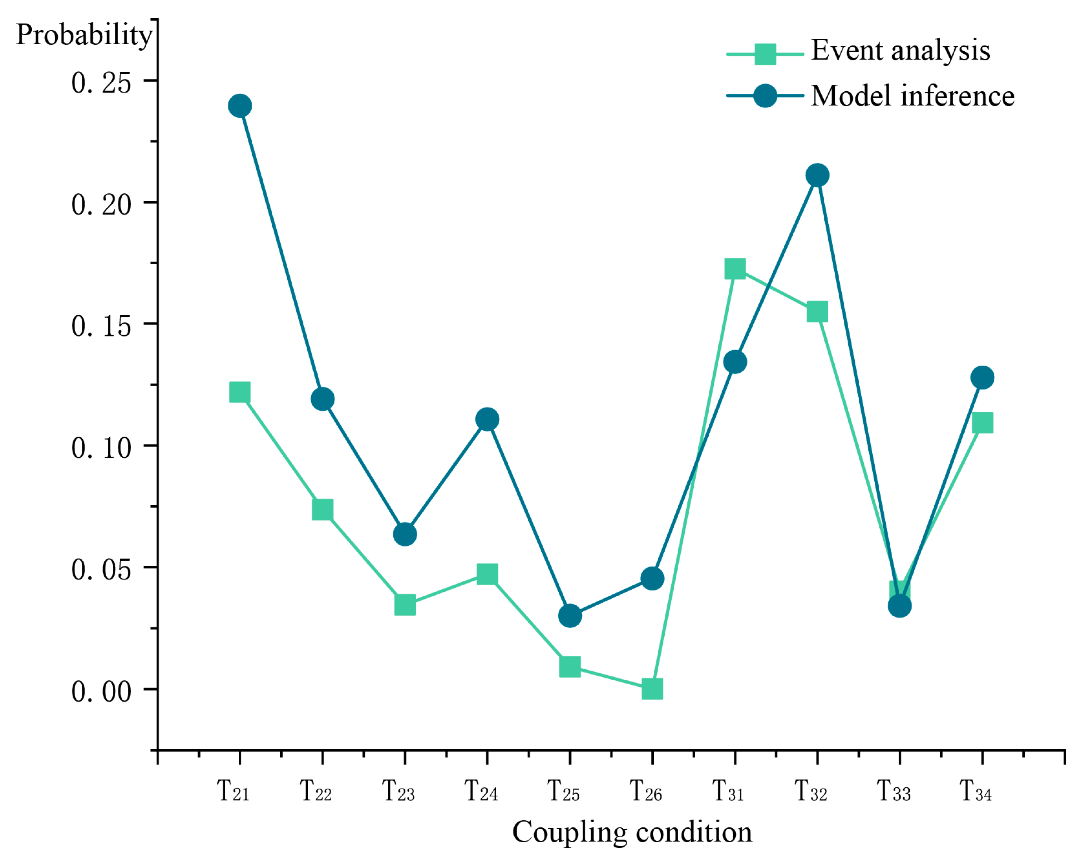
HFE is the result of a chain reaction of several factors. Sensitivity analysis studies the effect of small changes in the lower nodes of a model on the model parameters, which can help identify sensitive nodes in a BN [39]. In this study, a sensitive indicator (SI) [40] was used to analyze the dependence of nodes. $S{I}_{ij}$ expresses the rate of change in node $j$ being in an unfavorable state caused by the change of node $i$:

$$S{I}_{ij}=\frac{Pr(X_j=1|X_j=1)-Pr\left(X_j=1|X_i=0\right)}{Pr\left(X_j=1|X_i=0\right)}$$

(18)

where $X_i$ and $X_j$ are the states of the parent and child nodes, respectively. The extreme states of a node are described through 0 and 1, where 1 denotes an unfavorable state, and 0 denotes a favorable state. Then $Pr(X_j=1|X_j=1)$ is the probability that a child node is in an unfavorable state when the parent node is in an unfavorable state. $Pr\left(X_j=1|X_i=0\right)$ is the probability that a child node is in an unfavourable state when the parent node is in a favorable state. Considering the SI analysis of whether the team communication is smooth and the change in human error state as an example. When the probability of poor communication is 1.00, the probability of human error is 0.62. Meanwhile, when the team communication is smooth, the probability of human error is 0.15. Using Equation (18), the SI for operator error caused by team communication is calculated as (0.62 − 0.15)/0.15 = 3.13.

Based on the BN shown in Figure 5, we changed the state of any parent node and then calculated the SI of the child nodes connected to it according to Equation (18). Because there are five levels with node “HEP”, the total HEP for HFE under a certain combination is needed (the HEP expectation). It can be derived from Equation (19):

$$e={\sum }_i{x}_i·Pr\left(p=x_i\right)$$

(19)

where $x_i$ is the HEP reference value for each of the five levels.

Figure 6 shows the SI of nodes interacting with each other, where rows are parent nodes and columns are child nodes. Sensitive nodes are classified with SI = 3 as the threshold. For the SI between the factors, team communication openness ($F_5$) was more sensitive to team cooperative ($F_9$), training experience ($F_2$) was sensitive to team cooperative ($F_9$), and level of manipulation ($F_1$) was sensitive to mental state ($F_4$).With HEP as the observation node, spatial cognitive ability ($F_6$), team communication ($F_5$), task complexity ($F_8$), team cooperative ($F_9$), and control mode ($F_{16}$) are the sensitive nodes. The SI size determines its impact on the model output. Therefore, the probability of the HFE can be reduced by controlling the sensitive factors.

The impact of sensitive nodes on the model can be reflected in two ways: (1) the nodes directly and significantly impact HEP, such as team cooperation ($F_9$); (2) the nodes can determine the final HEP by influencing other nodes. For example, team communication affects HEP through team cooperation ($F_9$).

4.3. Validation

Several influencing factors often exist in human space missions [41]. According to Heinrich’s chain theory of accident causality [42], the failure of a single factor often does not lead to HFE. However, the failure of coupled factors causes the overall risk value of the operation to exceed the system design reliability level, which leads to HFE. The N-K model [43] has been widely used to analyze the effects of coupled factors on an entire system. The proposed ISM-BN model is likewise the result of a comprehensive consideration of the dependence between factors. Moreover, because the calculation principle of the N-K model considers the probability of HFE instead of the severity of the consequences, the risk coupling intensity derived from the N-K model can be regarded as the probability of HFE as assessed by the proposed HRA model. Therefore, the results of analyzing HFE using the N-K model can validate the ISM-BN model.

In this section, 52 incidents in “Accidents and Disasters in Human Space Flight” [44] are analyzed. Two HRA experts identified attributions according to the factors of [27] and classified them into four categories: individual, team, machine, and context, based on the factors belonging to them. Using the N-K model, risk coupling is classified into single-, double-, and multi-factor coupling (Figure 7).

$F_{vwxy}$ is denoted as the frequency of HFE occurrence under the factor coupling category, where $v, w, x, y$ represent the states of individual, team, machine, and context factors, respectively. The states of the four categories are defined from 0 through 1, where 0 indicates that the factor has not yet breached the defense of the subsystem, and 1 indicates that the factor has breached the defense of the subsystem. For example, F₀₀₀₀ indicates the frequency of events in which all four categories of factors—individual, team, machine, and scenario—have breached the system’s defenses. The frequency of factors coupled to trigger HFE can be counted, as shown in

Table 4. The frequency of events under different conditions.

Condition	Frequency	Condition	Frequency	Condition	Frequency	Condition	Frequency
F0000	0	F0010	0.0222	F0110	0.0222	F1101	0.0222
F1000	0.1333	F1100	0.0444	F0101	0	F1011	0.0444
F0010	0.0444	F1010	0.2	F0011	0.1556	F0111	0

.

Definition “.” indicates that a category of factors can be in either 0 or 1 state. According to the N-K model, the probability that the coupling of different categories of factors triggers HFE can be calculated. For example, F₀... denotes the probability of a failure event occurring when an individual factor has not yet breached the defense system, which is the single-factor coupling probability $\left(F_{0.\dots }=F_{0000}+F_{0100}+F_{0010}+F_{0001}+F_{0110}+F_{0101}+F_{0011}+F_{0111}=0.2904\right)$.

Next, the coupling strength T based on information entropy and coupled risk probabilities can be calculated. The more frequent the number of coupling, the higher the probability of coupling; the higher the coupling strength, the higher the associated risk. The coupling relationships involved include local and full coupling cases [45]. Equations (20) and (21) demonstrate the representative equations for two-factor and three-factor local coupling, and Equation (22) is the strength calculation equation for four-factor full coupling.

$$T_{21}=T_{\left(\mathrm{a},\mathrm{b}\right)}={\sum }_{v=1}^V{\sum }_{w=1}^W{F}_{vw}{\log }_2\left(F_{vw}/\left(F_{v\dots }\times F_{.w..}\right)\right)$$

(20)

$$T_{31}=T_{\left(\mathrm{a},\mathrm{b},\mathrm{c}\right)}={\sum }_{v=1}^V{\sum }_{w=1}^X{\sum }_{x=1}^Y{F}_{vwx}{\log }_2\left(F_{vwx}/\left(F_{v\dots }\times F_{.w..}\times F_{..x.}\right)\right)$$

(21)

$$T_4=T_{\left(\mathrm{a},\mathrm{b},\mathrm{c},\mathrm{d}\right)}={\sum }_{v=1}^V{\sum }_{w=1}^W{\sum }_{x=1}^X{\sum }_{y=1}^Y{F}_{vwxy}{\log }_2\left(F_{vwxy}/\left(F_{v\dots }\times F_{.w..}\times F_{..x.}\times F_{\dots y}\right)\right)$$

(22)

where “a” represents the individual factor, “b” represents the team factor, “c” represents the machine factor, and “d” represents the context factor. $v=1,2,\dots ,V;w=1,2,\dots ,W;x=1,2,\dots ,X;y=1,2,\dots ,Y$. $F_{vw}$ is the HEP (risk coupling strength) of coupling the individual factors and team factors. Because HFE in space missions is a rare event and full-factor coupling leads to HFE being even rarer, we analyzed the local risk coupling strength (including two- and three-factor coupling). As a result, the event analysis based on the N-K model is completed. The results are shown in

Table 5. The results of event analysis under different coupling conditions.

T21	T22	T23	T24	T25	T26	T31	T32	T33	T34
0.0091	0.0736	0.0346	0.0472	0.1219	0.0002	0.1727	0.1550	0.0402	0.0993

.

According to the ISM-BN model, the probability of HFE under the above coupling condition can be calculated in GENIE [46]. Based on Equation (19), the total HEP expectation for each coupling condition can be calculated in

Table 6. The results of model inference under different coupling conditions.

Condition	Very High	High	Medium	Low	Very Low	HEP Expectation
T21	0.5132	0.5255	0.5255	0.2435	0.0525	0.0301
T22	0.9999	0.9999	0.4555	0.2525	0.1601	0.1192
T23	0.9999	0.4816	0.2817	0.2525	0.0601	0.0636
T24	0.0003	0.0723	0.0002	0.1947	0.2321	0.1408
T25	0.0003	0.0721	0.1946	0.1946	0.2321	0.2397
T26	0.0002	0.9999	0.0003	0.2101	0.0409	0.0455
T31	0.2132	0.2255	0.2255	0.1625	0.2254	0.1345
T32	0.3069	0.3254	0.3254	0.3145	0.3435	0.2112
T33	0.5999	0.3817	0.0817	0.0525	0.0600	0.0342
T34	0.0003	0.0072	0.0003	0.1946	0.2159	0.1080

.

Pearson correlation analysis of the event analysis and model inference results showed a correlation coefficient of 0.757 ($p=0.011<0.0$5), indicating that the constructed model has a certain degree of accuracy. A comparison of the event analysis and model inference results is shown in Figure 8. The T-values of T₂₁, T₃₁, and T₃₂ individual–team–scenario are the largest, which fully demonstrate that human factors (individual and team) are the focus of future management. Only in the case of individual–team (T₂₁) coupling was T of two-factor coupling larger than T of three-factor coupling, indicating the complexity of factor coupling in space-teleoperation. T/HEP is positively correlated with the number of coupling factors, implying that controlling the occurrence of multi-factor coupling will be the focus of space-teleoperation management.

5. Conclusions

Herein, an HRA model is constructed for space teleoperation by integrating ISM and BN. The model is validated by analyzing human spaceflight-related events based on the N-K model. The findings highlight the priority direction for safety management in space teleoperation. In addition, the model can be continuously updated by extending the dataset. The conclusions are as follows:

(1)

The constructed model integrates data from expert judgment with experimental data, offering the potential for continuous model updates as more empirical data become available in the future.

(2)

Sensitivity analysis conducted using the HRA model shows that spatial cognitive ability ($F_6$), team communication ($F_5$), task complexity ($F_8$), team cooperative ($F_9$), and control mode ($F_{16}$) are HEP-sensitive nodes. Minor improvements in the involved factors can substantially reduce overall system risk.

(3)

Model validation shows that the occurrence of multi-factor coupling will be key for risk prevention. Moreover, human factors (individual and team factors) will be central to safety management.

The constructed HRA model considers the relationship between influencing factors and integrates expert judgment and experimental data. In this model, nodes are defined in terms of space teleoperation missions. Conditional probabilities are also based on teleoperation tasks. In the future, we can modify nodes through specific task scenarios, obtain the task data, and build an HRA evaluation model for more task scenarios using a similar approach.

References

1. Qi, W.; Wang, N.; Su, H.; Aliverti, A. DCNN based human activity recognition framework with depth vision guiding. Neurocomputing 2022, 486, 261–271. [Google Scholar] [CrossRef]
2. Ovur, S.E.; Zhou, X.; Qi, W.; Zhang, L.; Hu, Y.; Su, H.; Ferrigno, G.; De Momi, E. A novel autonomous learning framework to enhance sEMG-based hand gesture recognition using depth information. Biomed. Signal Process. Control 2021, 66, 102444. [Google Scholar] [CrossRef]
3. Zhao, J.; Lv, Y.; Zeng, Q.; Wan, L. Online policy learning-based output-feedback optimal control of continuous-time systems. IEEE Trans. Circuits Syst. II Express Briefs 2022, 71, 652–656. [Google Scholar] [CrossRef]
4. Tong, M.; Chen, S.; Niu, Y.; Wu, J.; Tian, J.; Xue, C. Visual search during dynamic displays: Effects of velocity and motion direction. J. Soc. Inf. Disp. 2022, 30, 635–647. [Google Scholar] [CrossRef]
5. Paglioni, V.P.; Groth, K.M. Dependency definitions for quantitative human reliability analysis. Reliab. Eng. Syst. Saf. 2022, 220, 108274. [Google Scholar] [CrossRef]
6. Liu, P.; Li, Z. Human error data collection and comparison with predictions by SPAR-H. Risk Anal. 2014, 34, 1706–1719. [Google Scholar] [CrossRef] [PubMed]
7. Hollnagel, E. Cognitive Reliability and Error Analysis Method (CREAM); Elsevier: Amsterdam, The Netherlands, 1998. [Google Scholar]
8. Gertman, D.; Blackman, H.; Marble, J.; Byers, J.; Smith, C. The SPAR-H human reliability analysis method. US Nucl. Regul. Comm. 2005, 230, 35. [Google Scholar]
9. Chang, Y.; Mosleh, A. Cognitive modeling and dynamic probabilistic simulation of operating crew response to complex system accidents. Part 2: IDAC performance influencing factors model. Reliab. Eng. Syst. Saf. 2007, 92, 1014–1040. [Google Scholar] [CrossRef]
10. Wang, L.; Wang, Y.; Chen, Y.; Pan, X.; Zhang, W.; Zhu, Y. Methodology for assessing dependencies between factors influencing airline pilot performance reliability: A case of taxiing tasks. J. Air Transp. Manag. 2020, 89, 101877. [Google Scholar] [CrossRef]
11. De Ambroggi, M.; Trucco, P. Modelling and assessment of dependent performance shaping factors through Analytic Network Process. Reliab. Eng. Syst. Saf. 2011, 96, 849–860. [Google Scholar] [CrossRef]
12. Adedigba, S.A.; Khan, F.; Yang, M. Process accident model considering dependency among contributory factors. Process Saf. Environ. Prot. 2016, 102, 633–647. [Google Scholar] [CrossRef]
13. Kim, Y.; Park, J.; Jung, W.; Jang, I.; Seong, P.H. A statistical approach to estimating effects of performance shaping factors on human error probabilities of soft controls. Reliab. Eng. Syst. Saf. 2015, 142, 378–387. [Google Scholar] [CrossRef]
14. Kabir, S.; Papadopoulos, Y. Applications of Bayesian networks and Petri nets in safety, reliability, and risk assessments: A review. Saf. Sci. 2019, 115, 154–175. [Google Scholar] [CrossRef]
15. Giudici, P. Bayesian data mining, with application to benchmarking and credit scoring. Appl. Stoch. Models Bus. Ind. 2001, 17, 69–81. [Google Scholar] [CrossRef]
16. Martins, M.R.; Maturana, M.C. Application of Bayesian Belief networks to the human reliability analysis of an oil tanker operation focusing on collision accidents. Reliab. Eng. Syst. Saf. 2013, 110, 89–109. [Google Scholar] [CrossRef]
17. Musharraf, M.; Hassan, J.; Khan, F.; Veitch, B.; MacKinnon, S.; Imtiaz, S. Human reliability assessment during offshore emergency conditions. Saf. Sci. 2013, 59, 19–27. [Google Scholar] [CrossRef]
18. Johnson, K.; Morais, C.; Patelli, E.; Walls, L. A data driven approach to elicit causal links between performance shaping factors and human failure events. In Proceedings of the European Conference on Safety and Reliability 2022, Dublin, Ireland, 28 August–1 September 2022; pp. 520–527. [Google Scholar]
19. Guan, L.; Abbasi, A.; Ryan, M.J. Analyzing green building project risk interdependencies using Interpretive Structural Modeling. J. Clean. Prod. 2020, 256, 120372. [Google Scholar] [CrossRef]
20. Xu, X.; Zou, P.X. Analysis of factors and their hierarchical relationships influencing building energy performance using interpretive structural modelling (ISM) approach. J. Clean. Prod. 2020, 272, 122650. [Google Scholar] [CrossRef]
21. Wu, W.-S.; Yang, C.-F.; Chang, J.-C.; Château, P.-A.; Chang, Y.-C. Risk assessment by integrating interpretive structural modeling and Bayesian network, case of offshore pipeline project. Reliab. Eng. Syst. Saf. 2015, 142, 515–524. [Google Scholar] [CrossRef]
22. Hou, L.-X.; Liu, R.; Liu, H.-C.; Jiang, S. Two decades on human reliability analysis: A bibliometric analysis and literature review. Ann. Nucl. Energy 2021, 151, 107969. [Google Scholar] [CrossRef]
23. Mkrtchyan, L.; Podofillini, L.; Dang, V.N. Methods for building conditional probability tables of bayesian belief networks from limited judgment: An evaluation for human reliability application. Reliab. Eng. Syst. Saf. 2016, 151, 93–112. [Google Scholar] [CrossRef]
24. Prvakova, S.; Dang, V. A Review of the Current Status of HRA Data; Paul Scherrer Institute: Villigen, Switzerland, 2014; pp. 595–603. [Google Scholar]
25. Podofillini, L.; Mkrtchyan, L.; Dang, V. Aggregating expert-elicited error probabilities to build HRA models. In Safety and Reliability: Methodology and Applications; CRC Press: Boca Raton, FL, USA, 2014; pp. 1119–1128. [Google Scholar]
26. Mosleh, A.; Bier, V.M.; Apostolakis, G. A critique of current practice for the use of expert opinions in probabilistic risk assessment. Reliab. Eng. Syst. Saf. 1988, 20, 63–85. [Google Scholar] [CrossRef]
27. Zhang, H.; Shanguang, C.; Wang, C.; Deng, Y.; Xiao, Y.; Zhang, Y.; Dai, R. Analysis of factors affecting teleoperation performance based on a hybrid Fuzzy DEMATEL method. Space Sci. Technol. 2024. [Google Scholar] [CrossRef]
28. Podofillini, L.; Dang, V.N. A Bayesian approach to treat expert-elicited probabilities in human reliability analysis model construction. Reliab. Eng. Syst. Saf. 2013, 117, 52–64. [Google Scholar] [CrossRef]
29. Atwood, C.L. Constrained noninformative priors in risk assessment. Reliab. Eng. Syst. Saf. 1996, 53, 37–46. [Google Scholar] [CrossRef]
30. Greco, S.F.; Podofillini, L.; Dang, V.N. A Bayesian model to treat within-category and crew-to-crew variability in simulator data for Human Reliability Analysis. Reliab. Eng. Syst. Saf. 2021, 206, 107309. [Google Scholar] [CrossRef]
31. Zhang, Z.-X.; Wang, L.; Wang, Y.-M.; Martínez, L. A novel alpha-level sets based fuzzy DEMATEL method considering experts’ hesitant information. Expert Syst. Appl. 2023, 213, 118925. [Google Scholar] [CrossRef]
32. Warfield, J.N. Developing interconnection matrices in structural modeling. IEEE Trans. Syst. Man Cybern. 1974, SMC-4, 81–87. [Google Scholar] [CrossRef]
33. Liu, J.; Wan, L.; Wang, W.; Yang, G.; Ma, Q.; Zhou, H.; Zhao, H.; Lu, F. Integrated fuzzy DEMATEL-ISM-NK for metro operation safety risk factor analysis and multi-factor risk coupling study. Sustainability 2023, 15, 5898. [Google Scholar] [CrossRef]
34. Swain, A.D.; Guttmann, H.E. Handbook of Human-Reliability Analysis with Emphasis on Nuclear Power Plant Applications. Final Report; Sandia National Lab. (SNL-NM): Albuquerque, NM, USA, 1983. [Google Scholar]
35. Groth, K.M.; Smith, C.L.; Swiler, L.P. A Bayesian method for using simulator data to enhance human error probabilities assigned by existing HRA methods. Reliab. Eng. Syst. Saf. 2014, 128, 32–40. [Google Scholar] [CrossRef]
36. Schneider, W.; Shiffrin, R.M. Controlled and automatic human information processing: I. Detection, search, and attention. Psychol. Rev. 1977, 84, 1. [Google Scholar] [CrossRef]
37. Zhang, M.; Zhang, D.; Yao, H.; Zhang, K. A probabilistic model of human error assessment for autonomous cargo ships focusing on human–autonomy collaboration. Saf. Sci. 2020, 130, 104838. [Google Scholar] [CrossRef]
38. Chen, H.; Zhao, Y.; Ma, X. Critical factors analysis of severe traffic accidents based on Bayesian network in China. J. Adv. Transp. 2020, 2020, 8878265. [Google Scholar] [CrossRef]
39. Li, C.; Mahadevan, S. Sensitivity analysis of a Bayesian network. ASCE-ASME J. Risk Uncertain. Eng. Syst. Part B Mech. Eng. 2018, 4, 011003. [Google Scholar] [CrossRef]
40. Lu, Y.; Wang, T.; Liu, T. Bayesian network-based risk analysis of chemical plant explosion accidents. Int. J. Environ. Res. Public Health 2020, 17, 5364. [Google Scholar] [CrossRef] [PubMed]
41. Bartone, P.T.; Roland, R.; Bartone, J.; Krueger, G.; Sciaretta, A.; Johnsen, B.H. Human adaptability for deep space exploration mission: An exploratory study. J. Hum. Performanc Extrem. Environ. 2019, 15, 2327–2937. [Google Scholar]
42. Manuele, F.A. Reviewing Heinrich. Prof. Saf. 2011, 56, 52–61. [Google Scholar]
43. Zhang, M.; Yu, D.; Wang, T.; Xu, C. Coupling analysis of tunnel construction safety risks based on NK model and SD causality diagram. Buildings 2023, 13, 1081. [Google Scholar] [CrossRef]
44. David, S. Disasters and Accidents in Manned Spaceflight; Springer Science & Business Media: Berlin, Germany, 2000. [Google Scholar]
45. Wu, B.-J.; Jin, L.-H.; Zheng, X.-Z.; Chen, S. Coupling analysis of crane accident risks based on Bayesian network and the NK model. Sci. Rep. 2024, 14, 1133. [Google Scholar] [CrossRef]
46. Zhang, X.; Mahadevan, S. Bayesian network modeling of accident investigation reports for aviation safety assessment. Reliab. Eng. Syst. Saf. 2021, 209, 107371. [Google Scholar] [CrossRef]
Figure 1. The framework of the method.
Machines 12 00524 g001
Figure 2. The qualitative structure of Bayesian network. (a) The hierarchical structure; (b) The topological structure.
Machines 12 00524 g002
Figure 3. First-stage update results for combination 1. (a) The prior probability distribution of θ; (b) The posterior probability distribution θ; (c) The posterior probability distribution HEP.
Machines 12 00524 g003
Figure 4. Second-stage update results for combination 1. (a) The prior probability distribution of θ; (b) The posterior probability distribution θ; (c) The posterior probability distribution HEP.
Machines 12 00524 g004
Figure 5. HRA model of space teleoperation.
Machines 12 00524 g005
Figure 6. Sensitive analysis of HRA model.
Machines 12 00524 g006
Figure 7. Factor coupling type.
Machines 12 00524 g007
Figure 8. The comparison of event analysis and model reference.
Machines 12 00524 g008