Abstract
Effective path planning is crucial for autonomous mobile robots navigating complex environments. The “global–local” coupled path planning algorithm exhibits superior global planning capabilities and local adaptability. However, these algorithms often fail to fully realize their potential due to low efficiency and excessive constraints. To address these issues, this study introduces a simpler and more effective integration strategy. Specifically, this paper proposes using a bi-layer map and a feasible domain strategy to organically combine the D*Lite algorithm with the Dynamic Window Approach (DWA). The bi-layer map effectively reduces the number of nodes in global planning, enhancing the efficiency of the D*Lite algorithm. The feasible domain strategy decreases constraints, allowing the local algorithm DWA to utilize its local planning capabilities fully. Moreover, the cost functions of both the D*Lite algorithm and DWA have been refined, enabling the fused algorithm to cope with more complex environments. This paper conducts simulation experiments across various settings and compares our method with A_DWA, another “global–local” coupled approach, which combines A* and DWA. D_DWA significantly outperforms A_DWA in complex environments, despite a 7.43% increase in path length. It reduces the traversal of risk areas by 71.95%, accumulative risk by 80.34%, global planning time by 26.98%, and time cost by 35.61%. Additionally, D_DWA outperforms the A_Q algorithm, a coupled approach validated in real-world environments, which combines A* and Q-learning, achieving reductions of 1.34% in path length, 67.14% in traversal risk area, 78.70% in cumulative risk, 34.85% in global planning time, and 37.63% in total time cost. The results demonstrate the superiority of our proposed algorithm in complex scenarios.
1. Introduction
Path planning technology is a key technology for autonomous mobile robots. In recent years, with the continuous development of robotics, path planning for robots has evolved from navigating flat, paved environments to handling more complex, unstructured environments [1,2]. In agriculture, robots are required to perform tasks such as operations and inspections in unstructured environments. In the military domain, robots maneuver through complex terrains, and optimized path planning significantly reduces the frequency of exposure to threats, thereby enhancing the safety of tactical maneuvers. Additionally, robots are extensively used in other hazardous environments, such as handling dangerous materials, mining operations, and post-disaster recovery. These applications further underscore the importance of path planning algorithms in terms of capability, efficiency, and adaptability.
Traditional path planning algorithms always aim at minimizing the path length [3]; however, in many real-world problems, the shortest path does not necessarily represent the optimal path. For example, in a combat scenario where robots may be attacked, path planning cannot be based on length alone. The shortest path may be the most dangerous and rugged, while the safest and flattest area may be the longest. Obviously, in real-world environments, only a combination of path lengths and environmental risks (or other costs of paths) can lead to a reasonable solution [4,5]. The study of path planning in rugged environments can help robots explore more complex application environments, and the study has high research value.
Path planning algorithms are broadly categorized into two types: global path planning and local path planning. The primary objective of global path planning is to identify a path from the starting point to the destination within a known environment. It strives to attain an optimal solution, with the accuracy of the path contingent upon the precision of environment acquisition. Noteworthy examples encompass the A* algorithm [6], the D* algorithm [7], the Dijkstra algorithm [8], and the RRT algorithm [9]. In contrast, local path planning focuses on considering local environmental information. This real-time path planning method operates based on dynamic information from the surroundings, exhibiting a high degree of robustness. Examples of local path planning algorithms comprise the Dynamic Window Approach (DWA) and Artificial Potential Field (AFP). Despite these advantages, such methods may not always yield optimal planning results or could even fail to discover a viable path due to the scarcity of global information.
The primary distinction between global and local path planning lies in the level of environmental information accessible to the robot. Global path planning becomes susceptible to errors when confronted with unknown obstacles in the environment. Therefore, researchers have proposed numerous hybrid algorithms to mitigate the limitations associated with single algorithms, particularly in scenarios involving large-scale maps with multiple dynamic obstacles. While this global–local coupling architecture significantly enhances performance in complex and dynamic environments, it also has limitations that result in a failure to fully harness the potential of the fusion algorithm.
Specifically, the current coupling method exhibits several problems. First, the traditional coupling approach is inefficient because global and local path planning use the same map, requiring frequent recalculation of nodes by both algorithms. This increases the computational load on the robot. Second, global path planning imposes excessive constraints on local path planning, such as inflection points and overly restricted areas. Furthermore, the majority of the global planning process typically occurs only once at the outset, causing the robot to rely heavily on local path planning to navigate through dynamic obstacles. A drastic change in the environment can quickly invalidate the data from global planning. Consequently, there is a pressing need for a novel global–local coupling architecture to address these problems.
In response to these challenges, this paper introduces a novel path planning method that integrates the D*Lite algorithm with the DWA, specifically designed to overcome the limitations identified earlier. We have developed a bi-layer map to reduce redundant node calculations across global algorithms, significantly enhancing overall system efficiency. Furthermore, by converting specific nodes recommended by global path planning algorithms into broader recommended regions, this method alleviates the constraint typically imposed by global path planning algorithms. This strategic transformation not only expands the operational space available for local planning algorithms but also prevents the emergence of inflection points, ensuring that the final path is closer to the trajectory of real robots. Additionally, to address the challenges of global planning path failure caused by environmental changes, this study uses the D*Lite algorithm as the global planning component of the fused algorithm. The D*Lite algorithm’s ability to reuse previous search information enables it to rapidly adjust and generate effective paths in response to environmental changes [4]. Moreover, enhancements to the cost functions of both the D*Lite and DWA algorithms ensure a broader range of environmental factors are considered, moving beyond mere path length to more effectively accommodate complex environments.
To validate the effectiveness of our proposed algorithm, we developed a custom map based on the peaks function, incorporating both static and dynamic obstacles and risks to simulate complex environments. The evaluation metrics included path length, frequency of traversing risk areas, accumulative risk, computational time for global planning, and total time cost. Comparative analysis conducted in environments with dynamic risks and obstacles showed that although our method, D_DWA, increased the path length by 7.43% compared to another global–local coupled method combining A* with DWA (A_DWA), it demonstrated significant advantages in key performance indicators: reduction in traversal through risk areas by 71.95%, decrease in cumulative risk by 80.34%, shortening of global planning time by 26.98%, and a reduction in overall time cost by 35.61%. Compared with another algorithm A_Q that has been verified to be effective in a real environment, D_DWA achieves reductions of 1.34% in path length, 67.14% in traversal risk area, 78.70% in cumulative risk, 34.85% in global planning time, and 37.63% in total time. These results not only highlight the efficiency and safety of D_DWA in navigating complex dynamic environments but also demonstrate its potential for extensive application in autonomous navigation systems.
The main contributions of this work can be summarized as follows:
- Developed a path planning approach that fuses the D*Lite algorithm with the DWA and introduced a bi-layer map approach to significantly reduce redundant node calculations and enhance overall system efficiency.
- Proposed a transformation of recommended nodes from global planning into feasible regions, which eased the constraints of global path planning on local path planning and introduced tailored short-term goals for these regions.
- Improved the cost functions of the D*Lite and DWA algorithms to encompass a wider range of environmental factors, thus enhancing the adaptability of the algorithms.
This paper is organized as follows. Section 2 reviews related works. Section 3 describes the improvements of the D*Lite algorithm and DWA algorithm. Section 4 presents the global–local fusion method proposed in this paper. Simulation results in Section 5 confirm the effectiveness of the fusion algorithm. Section 6 concludes this paper. Notations frequently used in this paper are collected in Table 1.

Table 1.
Notation system.
2. Related Works
2.1. Path Planning in Complex Environments
In recent years, path planning for robots in complex environments has attracted significant attention. These planning algorithms must consider not only the path length but also a variety of environmental factors to ensure that the paths are both effective and safe.
Kim et al. aid mobile navigation by constructing 3D topographic cloud maps of chaotic environments. Their proposed methodology reduced human intervention and the time required for data collection and processing [10]. However, this study simplifies complex environments into binary feasible and infeasible regions, neglecting the potential for robots to traverse certain regions.
To extend the robot’s movement ranges into 3D spaces, Tarokh utilized terrain roughness and curvature to achieve path planning for a highly maneuverable robot in the rugged terrain of Mars [11]. Li et al. improved the Rapidly exploring Random Tree (RRT) algorithm by considering constraints such as terrain height variation and flatness. This was achieved by establishing a 3D environment model for a mobile robot navigating complex rugged terrain [12]. Carvalho et al. developed a method for 3D traversability analysis and path planning in forest environments by utilizing terrain gradients and obstacle detection from 3D point cloud maps to optimize path selection [13]. Visca et al. improved an energy-based path planning approach for off-road scenarios, optimizing energy-efficient routes through uneven terrains [14].
Given the variety of evaluation methods for path planning in complex environments, which encompass everything from terrain slope and roughness to the robot’s energy consumption, it becomes essential to establish a unified evaluative metric. This work proposes “risk” as a potential comprehensive metric that integrates these factors. Although this study does not implement the integration, “risk” offers a framework that could accommodate a broader range of application scenarios, enhancing the evaluation of paths and ensuring the robustness and safety of path planning.
2.2. Global–Local Coupling Algorithm
Global–local coupled path planning represents an effective strategy to address the challenges of path planning in complex environments. This methodology compensates for the limitations inherent in relying on global or local planning algorithms by combining their strengths. It enhances the efficiency and robustness of path planning, making it particularly suited for dynamic and unpredictable settings.
Zhang et al. employed global path planning to chart a linear path connecting the starting point and the center of the search area. In case of the detection of a suspicious target, they transitioned to a distinct local path planning mode, thereby enhancing the efficacy of the search task [15]. Wang et al. used global path planning to generate sparse path points, subsequently integrating local path planning to circumvent unforeseen obstacles during path planning for autonomous surface vehicles in real geographical environments [16]. Liu et al. proposed a new fusion algorithm of the jump-A* algorithm and the DWA, which can effectively improve the smoothness and global optimality of the path [17]. Wang et al. advanced the field by adopting an improved particle swarm algorithm, along with an improved artificial potential field method, to accomplish path planning and, ultimately, to achieve dynamic obstacle avoidance in complex sea areas [18]. Jian et al. introduced a scheme incorporating the improved A* algorithm with a local path planner to realize global–local coupled two-phase paths. The effectiveness of this approach was assessed through simulations in an environment [19]. Additionally, Song et al. proposed a global dynamic path planning method based on the improved A* algorithm and dynamic window approach, showcasing notable efficiency and real-time performance [20]. Ji, in an effort to endow the robot with local obstacle avoidance ability based on the global optimal path, combined the optimized A* algorithm with the DWA, resulting in a fusion algorithm that harmonizes global and local path planning. The findings indicated a considerable improvement in the robot’s real-time obstacle avoidance ability when guided by the optimal path [21]. Sun et al. proposed a random path planning method based on the fusion of the A* algorithm and DWA, which ensures that random obstacles are avoided in real time based on the globally optimal path [22]. These methods have been shown to significantly improve the capabilities and adaptability of path planning algorithms. However, despite these advancements, current coupled methods still exhibit limitations that require further study, which are as follows:
- (1)
- The algorithms mentioned above do not optimize the number of nodes used by the global planning algorithm, which subsequently guides the local planning algorithm. In some scenarios, using a detailed map for global path planning is unnecessary and results in undue computational costs in large-scale environments. Therefore, it is essential to specifically optimize the global path planning map to reduce the number of nodes utilized, which is one of the topics this article addresses.
- (2)
- Global planning imposes excessive restrictions on local planning algorithms; global planning frequently enforces strict constraints on local planning, requiring local routes to adhere to globally defined routes or nodes [16,17,18,19,20,21,22]. This can result in unnecessary detours and increased path length in the local path planning algorithm. Therefore, it is crucial to explore methods to mitigate these constraints in order to fully utilize the capabilities of local path planning.
- (3)
- The global path may fail in dynamic environments: The paths generated by the global planning algorithms mentioned above may become obsolete in rapidly changing environments. In such cases, previously computed global planning data must be discarded, leading to a waste of computational resources. Therefore, it is essential to adopt measures to minimize the wastage of computational resources.
To address these identified limitations, this paper proposes corresponding improvement measures. Table 2 outlines the limitations and improvement strategies, clearly illustrating the proposed method.

Table 2.
Overview of limitations and proposed improvement strategies.
Therefore, this study refines the global–local path planning architecture to enhance its adaptability and precision in dynamic environments. This paper proposes solutions to overcome the existing limitations, offering a more efficient path planning approach.
3. Optimizing the D*Lite and DWA Algorithms
This section describes the traditional D*Lite algorithm and DWA algorithm. Furthermore, this section describes the method of optimizing the cost function of these two algorithms in this paper, to improve the ability of the D*Lite algorithm and DWA algorithm to cope with complex environments.
3.1. Overview of the D*Lite Algorithm
The D*Lite algorithm [22] is an improved incremental algorithm based on the Lifelong Planning A* algorithm (LPA*), which has been widely used for path planning in unknown and dynamic environments [23,24,25] and is able to reuse information from previous searches in order to find effective paths at a much faster rate than solving each search task from scratch.
The D*Lite algorithm is similar to the LPA* algorithm in that it searches in the opposite direction from LPA*, facilitating pathfinding from different starting points. In the D*Lite algorithm, s represents a node on the map, and S is the set of all nodes (). Succ(s) denotes the set of successor nodes to node s and Pred(s) denotes the set of predecessor nodes. g(s) represents the estimated cost from node s to the target node, determined by the value of rhs(s); the mathematical expression for rhs(s) is:
In Equation (1), sgoal denotes the target node and c(s, s′) denotes the cost from node s to node s′ (which is usually estimated using the distance).
Typically, g(s) is assigned through rhs(s). Additionally, under certain conditions (see the D*lite algorithm), we make g(s) = rhs(s), indicating that the rhs(s) is a one-step forward-looking value based on the g(s). For node s, rhs(s) is updated first, followed by an update to g(s). A change in g(s) for node s immediately affects pred(s), while a change in rhs(s) does not affect pred(s).
Both g(s) and rhs(s) serve as estimates for the shortest distance from node s to sgoal. However, their values may differ, and based on the difference, the states of the nodes are categorized into three classes. (1) When g(s) = rhs(s), the state of node s is locally consistent. (2) When g(s) > rhs(s), the state of node s is locally overconsistent. (3) When g(s) < rhs(s), the state of node s is locally underconsistent.
D*Lite initiates its search from the sgoal by expanding the node with the smallest k value in the priority queue and adds neighboring nodes or nodes with state changes to the priority queue through processing until the termination condition is satisfied. After this, the robot can reach the sgoal following the direction with the smallest cost. The k value is defined as follows:
Here, k(s) contains two parts: k1(s) and k2(s). When comparing, k1(s) is prioritized; if k1(s) values are identical, then k2(s) is compared (see the D*lite algorithm). The h(s,sstart) represents the heuristic value of the distance from node s to sstart. Since the sstart can be changed, a correction variable, km, is added to the k1 to ensure consistency. The definition of km is shown in Equation (5), where slast refers to the previous position of sstart.
3.2. Improving the D*Lite Algorithm Based on Environmental Information Weight
The traditional D*Lite algorithm expresses path cost in terms of distance. However, this paper aims to improve the D*Lite algorithm by enabling it to consider environmental information associated with the selected path. Specifically, a risk value r(s) is integrated into the cost function. Consequently, the revised cost function is proposed to evaluate paths based on their associated risk values.
Here, cdis(s, s′) denotes the length cost in the conventional D*Lite algorithm. λ1 is the weight that ensures consistency between cdis(s, s′) and r(s). It is worth noting that c(s, s′) is used to evaluate the value of selecting node s in , Therefore, when calculating c(s, s′), the value of r(s) should be used instead of r(s′).
For the purpose of enhancing the accuracy of the heuristic function, this study refines the heuristic function, denoted as h(s, sstart), drawing inspiration from Ref. [26]. The improved h(s, sstart) is presented as follows:
In Equation (7), (xstart, ystart) represents the position coordinates of sstart, and (xs, ys) represents the position coordinates of the node s.
3.3. Overview of the DWA Algorithm
The DWA algorithm is a fundamental local path planning algorithm. This algorithm’s process entails constructing an initial kinematic model of the robot, followed by creating a velocity space that includes linear and angular velocities. Subsequently, an evaluation function is employed to assess each velocity pair (v, w), enabling the algorithm to iteratively select the optimal velocity for the robot’s motion. This cyclic process continues until the goal is successfully reached [27].
3.3.1. Kinematics Model of Mobile Robot
In the DWA algorithm, establishing a robot kinematic model is the basis for simulating the robot’s motion trajectory. Assuming the robot travels at a pair of speeds (v, w), the trajectory can be either a curved segment or a line segment. The robot kinematics model is as follows:
Here, xr and yr represent the robot’s coordinate information at time t, while θ correspond to direction angles of the robot at time t. The variables v and w symbolize the robot’s linear and angular velocities.
3.3.2. Establishing Velocity Space
By utilizing the robot’s kinematic model, it becomes feasible to compute the robot’s trajectory. A velocity space is established to encompass velocities available for the robot’s selection, and subsequently, the optimal velocity is determined through the evaluation function. The robot continuously selects the optimal velocity until it successfully reaches the goal.
The velocities within this space should adhere to both the limitations of the robot itself and the constraints imposed by the environment:
(1) The velocity should fall within the range of the robot’s maximum and minimum velocities.
Here, vmin and vmax denote the robot’s minimum and maximum linear velocities, respectively. Similarly, wmin and wmax represent the robot’s minimum and maximum angular velocities.
(2) The velocity should adhere to the acceleration and deceleration capabilities of the robot.
where vc and wc represent the current linear and angular velocities, respectively, and stand for the maximum acceleration and maximum deceleration of the linear velocity, and correspond to the maximum acceleration and maximum deceleration of the angular velocity of robot.
(3) The robot’s speed is restricted to prevent collisions with obstacles.
where dist(v, w) represents the closest distance from the robot to the obstacle along the trajectory corresponding to the current speeds v and w.
Based on the aforementioned constraints, the robot’s ultimate velocity space emerges as the intersection of the three previously defined velocity spaces. Consequently, the robot’s final velocity is determined as follows.
3.4. Improving the DWA Algorithm Based on Environmental Information Weight
Similar to D*Lite, DWA should not treat the risk region as either an obstacle or an obstacle-free zone. Instead, the robot can select a low-risk path from this region, which requires changing the evaluation function of the traditional DWA. The modified evaluation function is as follows:
In Equation (15), α, β, γ, and λ2 are weights, where a higher weight corresponds to a greater dominant effect. The symbol ρ denotes the normalization process. The function heading(v, w) refers to the evaluation of the azimuth angle, which evaluates the angle between the orientation angle at the end of the robot’s trajectory and that of the robot’s position relative to the goal. The function dist(v, w) provides a distance evaluation; it is set to a constant value when no obstacle is present. The function velocity(v, w) is the velocity evaluation function to expect the agent to move at a high velocity. Lastly, r(sr) represents the risk value at the agent’s current position, as defined in Section 3.1.
In the formula, θ represents the angle between the orientation angle at the end of the robot’s trajectory and the orientation from the robot’s position to the goal. disttmp is the distance constant employed to ensure that dist(v, w) does not overly influence the result when no obstacles surround the agent. d_max denotes the distance between the end of the agent’s trajectory and the nearest obstacle.
Taking heading(v, w) as an example, the normalization method is as follows:
Here, Tr represents the total number of trajectories, while tr denotes the current trajectory. Among all trajectories, the one with the highest evaluation function value is considered the optimal choice.
4. Global–Local Fusion Method
The previous section mentioned that the current approach to fusing global and local path planning algorithms is computationally inefficient, leading to the double-counting of nodes. Moreover, dynamic environments heavily rely on local path planning, and there are significant limitations in the global path planning algorithm. To alleviate these problems, this section introduces our proposed approach for fusing global and local algorithms. Specifically, this section covers environmental modeling, the bi-layer map processing methodology, feasible region and temporary goal determination, and finally, a general overview of the proposed fusion method.
4.1. Environmental Modeling
To meet the requirements of robot path planning in complex environments, this study extends traditional algorithms to evaluate multiple environment dimensions, rather than relying solely on distance on a two-dimensional map as the cost. In this paper, riskiness is used as a parameter to characterize the third dimension of a robot’s environment. Here, riskiness is a generalized concept that can be specified using parameters such as altitude, terrain ruggedness, energy consumption costs, and other relevant factors in a real-world environment.
The working environment of the robot is simulated using the peaks function, which models both high and low peaks, as well as canyons, within a confined area. This environment serves as a comprehensive validation for the path planning algorithm’s capabilities.
In this paper, a region of the peak function’s domain is employed to create the risk map. The variables x and y are both limited to the interval [−3, 3] and are proportionally scaled to depict the driving risk on a 200 × 200 m2 map. The peak function is defined as follows:
where x and y represent the horizontal and vertical coordinates in the right-angle coordinate system, respectively. R(x, y) represents the risk value corresponding to the coordinate position. The scaling method is as follows:
where x1 and y1 denote the horizontal and vertical coordinates after the change of coordinates, and R(x1, y1) denotes the risk value after the change of coordinates. After scaling, both x1 and y1 are restricted to the interval [1, 200].
The risk of a 200 m × 200 m environment is assessed using a transformed risk function. The area is divided into 200 × 200 grids, each measuring 1 m × 1 m, and each grid represents a node in the path planning process. The processed value of the risk (after rounding and absolute value operations) at the top-right vertex of each grid is then used to estimate the risk level of that grid. The values of 1, 2, and 3 indicate different risk levels, with 0 indicating no risk at all and 4 indicating that the grid represents an obstacle and cannot be traversed. The risk values are defined as follows:
Here, r(s) represents the risk level of node s. The variables x1 and y1 correspond to the horizontal and vertical coordinates of any point within the region of node s, respectively. In this context, ceil(x) is an upward rounding function, and round(x) is a standard rounding function.
In order to explicitly express the environment and path, the risk information is converted into different grayscale values (GV) ranging from 0 to 255, when GV = 0 indicates no risk (white) and GV = 255 signifies an obstacle (black). Different grayscale values indicate varying levels of risk, with higher values corresponding to higher risk levels, as shown in Figure 1.
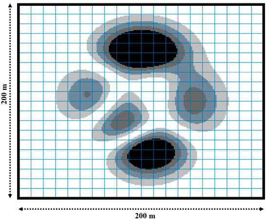
Figure 1.
Environmental modeling.
4.2. Bi-Layer Map Processing Methodology
Fine modeling of the environment tends to introduce a large number of nodes. The aforementioned environment map contains 40,000 nodes within a 200 m × 200 m area. If both global and local path planning utilize fine maps, this can result in wasted computational efficiency. Additionally, for the fusion path planning algorithm, global planning generates finer paths on detailed maps, potentially constraining the capabilities of local path planning and introducing unnecessary turns for local planning. Therefore, we propose the use of bi-layer maps for fusion path planning algorithms, which enhances planning efficiency while still fully utilizing the capabilities of the local planning algorithm.
The D*Lite algorithm in this paper provides guidance for the DWA, and it is not necessary to use fully accurate maps. The fusion algorithm proposed in this paper utilizes bi-layer maps. The global D*Lite algorithm employs processed coarse maps for path planning, providing guidance for local path planning. Subsequently, the DWA uses fine maps for further path planning.
In this study, the detailed map discussed in Section 4.1 is transformed into a coarse map. This coarse map is combined with the detailed map to create a bi-layer map for path planning. Specifically, the risk map generated in Section 4.1 is uniformly divided into square grids, each measuring 10 m × 10 m. The risk values of 100 nodes within each grid are then averaged to determine the risk level of the coarse map. In this way, a map with 200 × 200 nodes is converted into a 20 × 20 nodes coarse map. The risk level value of the coarse map is defined as follows:
where r(sc) represents the risk level value of the coarse map node sc. Additionally, si represents the i-th subpoint out of the 100 subpoints corresponding to node sc. The resulting bi-layer map is shown in Figure 2.
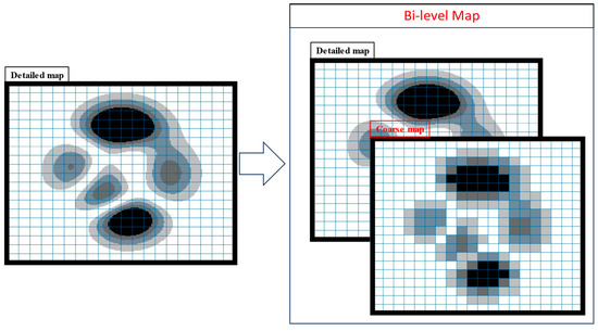
Figure 2.
The bi-layer map.
4.3. Feasible Region and Short-Term Goals
Using coarse maps for global path planning to guide local path planning algorithms can improve computational efficiency. Another key aspect of enhancing algorithm efficiency is how local path planning algorithms can better leverage the information provided by globally planned paths. This section describes the valuable information that global planning paths provide to local path planning algorithms, which includes feasible domain constraints and short-term goals.
Coarse maps for global path planning reduce the constraints imposed on local path planning by defining each node of a coarse map as a region. That is, the global path planning algorithm delineates a feasible region, and local path planning only needs to select the optimal solution within that region. However, the coarse map grid could cause this region to be point connected; for example, when selecting a diagonal path region, nodes are connected to each other by only one point. Therefore, this study adopts the envelope of the global path planning path as the limiting range for local path planning. As shown in Figure 3a, the red grids represent the large grids selected by the global path planning algorithm. These grids are numbered on the coarse map to indicate the forward direction, while the feasible region for the local path planning algorithm is depicted in blue.
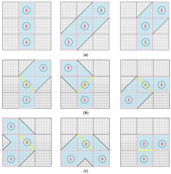
Figure 3.
The feasible region and short-term goals are determined by global path planning algorithm. (a) Feasible region delineated by the envelope under different scenarios. (b) Intersection lines serve as short-term goals (occurs when the direction of feasible regions shifts to adjacent directions). (c) Short-term goals in other scenarios.
Setting short-term goals is a prevalent strategy in local–global fusion path planning, significantly reducing the risk of the local path planning algorithm becoming trapped in a local optimum. In this study, we employ the inflection points of the feasible region as short-term objectives. Specifically, the agent’s feasible region encompasses eight directions, and when the direction of the feasible region transitions to any two adjacent directions, the intersection line of these two areas is chosen as a short-term goal. This approach helps the algorithm generate smooth paths. When the feasible region no longer changes direction and the goal becomes available, the goal is selected as the short-term goal. In other scenarios, the short-term goal is defined as the perpendicular lines drawn from two of the four vertices within the last large grid of the feasible region. As shown in Figure 3b,c, the short-term goals are represented by the yellow line segments.
4.4. Overview of the Fused Algorithm
The pseudocode of the fused algorithm is shown in Algorithm 1. Figure 4 presents the map processing workflow as exemplified through a specific instance. In this diagram, solid arrows depict both the processing sequence and the transfer of information, whereas dashed arrows indicate the transfer of information exclusively. The module proposed in this study is indicated in red font. During the path planning process, the D*Lite algorithm recommends feasible domains and temporary goals based on coarse maps. Subsequently, the DWA dynamically plans paths within these domains. When the next region is reached, the D*Lite algorithm leverages its incremental computational capabilities to update the recommended regions, and then the DWA plans the paths to next region. This process is iterated continuously until the goal is found. It is important to note that, starting from the second invocation of the D*Lite algorithm, it utilizes information from previously computed data to determine the feasible region. This characteristic is intrinsic to D*Lite itself and significantly improves computational efficiency. This attribute is one of the primary reasons for selecting the D*Lite algorithm as the global path planning algorithm in this paper.
| Algorithm 1. The pseudocode of fused algorithm. |
| 1: Input: sstart, sgoal, detailed map |
| 2: Output: path |
| 3: (xr, yr) = start_coords |
| 4: (xg, yg) = goal_coords |
| 5: ΔD = Define threshold distance |
| 4: while distance((xr, yr), (xg, yg)) > ΔD do: |
| 5: mapcoarse = bi-layer_map_processing(mapdetailed) |
| 6: nodes = improved_D*Lite((xr, yr), mapcoarse) |
| 7: region = calculate_feasible_region(nodes) |
| 8: short-term goal = calculate_short_term_goals(region) |
| 9: while distance((xr, yr), short-term goal) > ΔD do: |
| 10: (v, w) = improved_DWA((xr, yr), velocity, short-term goal, mapdetailed) |
| 11: (xr, yr), (v, w) = update_position_velocity((xr, yr), (v, w)) |
| 12: end while |
| 13: end while |
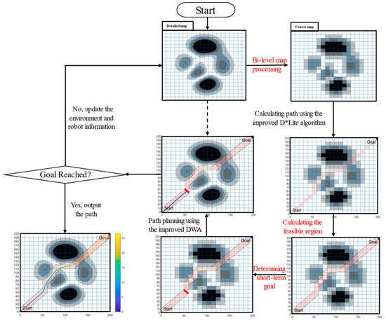
Figure 4.
Flowchart of the fused algorithm.
5. Simulation and Analysis
The traditional D*Lite algorithm, the improved D*Lite algorithm, the traditional DWA, the A* and DWA fusion method (A_DWA, which can handle environmental risks and has good dynamic performance, as described in [21]), and the fusion algorithm proposed in this paper are employed for path planning experiments. Both the traditional D*Lite algorithm and the improved D*Lite algorithm execute path planning on the coarse map, aiming to showcase the improved D*Lite algorithm’s ability to jointly consider risk and distance. The comparison among the traditional DWA, the improved DWA, the A* and DWA fusion algorithm, and the proposed algorithm reflects not only the global optimal ability and dynamic planning ability of the algorithm designed in this paper but also the enhanced algorithm efficiency.
All simulations are performed on a PC with Intel i7 2.3 GHz and 16 GB RAM, run by MATLAB R2022b. The experiments were performed in the risk map mentioned above. Table 3 shows the experimental parameters.

Table 3.
Experimental parameters.
5.1. Static Environment
In order to fully test the performance of the algorithm, we placed a number of obstacles that appeared suddenly on the map during the test; these obstacles were not surrounded by other risk level grids. There are two types of static simulation environments, which are as follows:
(A) The environment with only regional risk and no additional obstacles.
(B) An environment where obstacles are added to the planned path in environment (A), allowing the algorithm to replan the path and observe the performance.
The path planning results of the traditional D*Lite algorithm (Figure 5) and the improved D*Lite algorithm (Figure 6) on the coarse map are shown. Additionally, the results for the traditional DWA (Figure 7), the improved DWA (Figure 8), the fused algorithm of A* and DWA (Figure 9), and the proposed fusion algorithm of D*Lite algorithm and DWA (Figure 10) on the bi-layer map are presented.
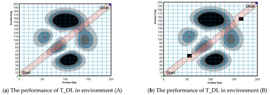
Figure 5.
The performance of T_DL for path planning in static environment.
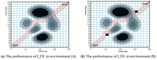
Figure 6.
The performance of I_DL for path planning in static environment.
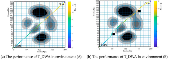
Figure 7.
The performance of T_DWA for path planning in static environment.
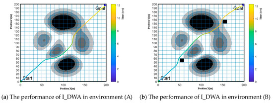
Figure 8.
The performance of I_DWA for path planning in static environment.
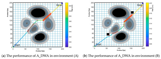
Figure 9.
The performance of A_DWA for planning path in static environment.
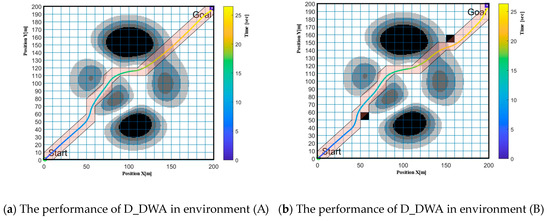
Figure 10.
The performance of D_DWA for planning path in static environment.
In Figure 5, Figure 6, Figure 7, Figure 8, Figure 9 and Figure 10, the start and the goal locations for all cases are set as sstart = (xstart, ystart) = (0, 0), and sgoal = (xgoal, ygoal) = (195–200, 195–200). The circle located in the lower-left corner of each figure represents the starting point, and the blue box in the upper-right corner represents the goal. The light red area indicates the recommended area based on the D*Lite algorithm, and the colored lines are the paths searched by the DWA. The color of the lines indicates the time cost by the algorithms, thereby demonstrating the real-time efficiency of the algorithms. The red circles indicate the key points planned by the A* algorithm in A_DWA. The gray-colored grids represent the driving risk for the agent. Grids with risk levels 0, 1, 2, and 3 are passable, while grids with risk level 4 are obstacles and cannot be traversed by the agent.
To visually compare the performance of the algorithms in various aspects, the following abbreviations are defined for the concepts: the length of the path (LOP), the number of risk grids the planned path passes through (NORG), the accumulation of the risk of the grids the planned path passes through (AROG), the global planning time in the fusion algorithm (GT), and the time cost for the algorithms (Time). The traditional D*Lite algorithm (T_DL), the improved D*Lite algorithm (I_DL), the traditional DWA (T_DWA), the improved DWA (I_DWA), the fused algorithm of A* and DWA(A_DWA), and the proposed algorithm in this paper (D_DWA) are compared based on five specific criteria, as shown in Table 4, Table 5, Table 6 and Table 7. Among them, since the T_DL and the I_DL algorithm plan the regional paths according to the coarse map (20 × 20), it is not possible to calculate the LOP, and the NORG and AROG of these two algorithms only calculate the number of large grids in coarse maps. In addition, the T_DWA does not consider the road risk level and directly traverses the risk area, so the path length has no reference meaning and is not the object of comparison.

Table 4.
Results of the different algorithms in environment (A).

Table 5.
Results of the different algorithms in environment (B).

Table 6.
Data comparison for the three algorithms in (A) environment.

Table 7.
Data comparison for the three algorithms in (B) environment.
As shown in Figure 5 and Figure 6, all scenarios can reach the goal. However, T_DL (Figure 5) does not consider the risk, and although it can avoid obstacles on the path, it directly traverses the high-risk area. On the other hand, I_DL (Figure 6) avoids unnecessary high-risk areas and yields a higher-quality path. I_DL provides a global solution in the risk environment, reducing NORG by 57% and AROG by 64% compared to the T_DL in environment (A). When obstacles are introduced, I_DL reduces NORG by 50% and AROG by 64% compared to T_DL. Therefore, I_DL significantly outperforms T_DL. Both algorithms have comparable time costs.
As shown in Figure 7, Figure 8, Figure 9 and Figure 10, all algorithms can reach the goal. The T_DWA (Figure 7) directly traverses areas with high risk levels. The I_DWA (Figure 8) can plan paths through the area with low risk while avoiding obstacles. In environment (A), the NORG of the I_DWA increases by 25% compared with T_DWA. This is because the T_DL directly traverses the high-risk grids, while the I_DWA explores part of the low-risk grids with risk level 1 to maintain the speed and driving angle of the agent. Despite the increase in NORG, the AROG decreases by 11%, indicating higher path safety. In environment (B), using I_DWA results in a 25% reduction in NORG and a 30% decrease in AROG, while maintaining a similar LOP and time cost to that of T_DWA. The path quality of I_DWA is significantly superior to that of T_DWA.
In terms of path quality, D_DWA shows more improvement compared to I_DWA, while A_DWA demonstrates less improvement and exhibits erratic performance. As can be seen from Table 6 and Table 7, the LOP of I_DWA, A_DWA, and D_DWA do not differ significantly in either environment (A) or environment (B). In environment (A), A_DWA’s NORG and AROG decrease by 20% and 12% relative to I_DWA, respectively. Meanwhile, D_DWA achieves a remarkable reduction of 44% in NORG and 36% in AROG. In environment (B), A_DWA experiences a 14% increase in NORG and a 6% increase in AROG relative to I_DWA, and the path quality is slightly worse. This is primarily attributed to the global algorithm A*, which strictly constrains the actions of local planning algorithms when obstacles are encountered. On the other hand, D_DWA achieves a 39% reduction in NORG and a 35% reduction in AROG relative to I_DWA. Regarding time cost, A_DWA takes 27.4 times and 34.4 times as long as I_DWA in environment (A) and (B), respectively. In contrast, D_DWA exhibits a significantly lower time cost, with ratios of only 2.0 and 2.1 times. The main reason for this phenomenon lies in the difference in time consumed by the global planning algorithm. As shown in Table 6 and Table 7, the GT for D_DWA is much smaller than that for A_DWA. This difference in time is comprised of two main factors: on one hand, the global planner D*Lite consumes less time than the A* algorithm; on the other hand, the bi-layer map significantly reduces the time cost of global planning by decreasing the number of map nodes (from 200 × 200 = 40,000 to 20 × 20 = 400). According to an experiment conducted by the authors, the time expenditure of the global planner D*Lite without bi-layer map processing for D_DWA is 59.28 s and 57.19 s for environment (A) and (B), respectively, which is reduced to 1.2 s and 1.09 s after applying bi-layer map processing.
When comparing the same global–local fusion algorithm, D_DWA, with A_DWA, it becomes evident that D_DWA holds a significant advantage. In environment (A), D_DWA reduces NORG by 29.6%, AROG by 27%, GT by 99.7%, and Time by 92.5% compared to A_DWA, albeit with a 1.3% increase in LOP. In environment (B), although LOP increases by 1.2% when comparing D_DWA to A_DWA, NORG decreases by 46.7%, AROG decreases by 39.3%, GT decreases by 99.7%, and Time decreases by 93.8%.
5.2. Dynamic Environment
In the dynamic environment experiment, two cases are considered. Figure 11 depicts the simulated environment for Case 1 and Case 2. As before, the circle in the lower-left corner represents the starting point for path planning, the blue box in the upper-right corner represents the goal, and the gray grid indicates the regional risk level. The pink line shows the obstacle’s direction of movement. The varying colors on the color bar to the right represent the time durations consumed by both the algorithms and the obstacles. The other elements in the figure are consistent with Section 5.1. The definitions of the case are as follows:
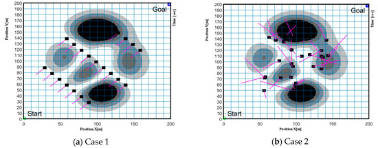
Figure 11.
Dynamic environment.
Case 1: Uniform obstacle
As shown in Figure 11a, the environment includes 20 dynamic obstacles that move toward the lower left at a speed of 0.1 m/s.
Case 2: Random obstacles
As shown in Figure 11b, the environment includes 30 dynamic obstacles. To test dynamic performance, the obstacle locations are randomly set within an x range of 50 to 150 and a y range of 50 to 150. The obstacle velocities are randomly set in a range from 0.0 m/s to 0.25 m/s.
Case 1 was conducted once, and Case 2 was repeated 10 times. Figure 12, Figure 13 and Figure 14 show the trajectory results for I_DWA, A_DWA, and D_DWA in both Case 1 and Case 2. Figure 12b, Figure 13b, and Figure 14b show the trajectories of the agent 10 times only. Table 8 contains the LOP, NORG, AROG, Time, and GT data for the three algorithms in Case 1. Table 9 lists the average length of the path (A_LOP), the average number of rough grids (A_NORG), the average accumulated risks of agent (A_AROG), the average Time (A_Time), and the average GT (A_GT) for the three algorithms in Case 2.
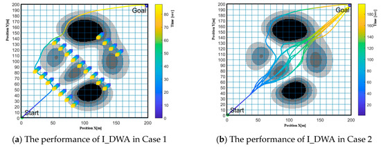
Figure 12.
The performance of I_DWA for planning path in dynamic environment.
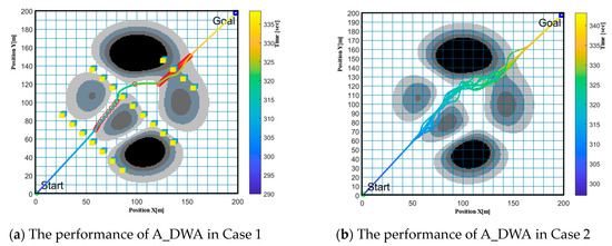
Figure 13.
The performance of A_DWA for planning path in dynamic environment.
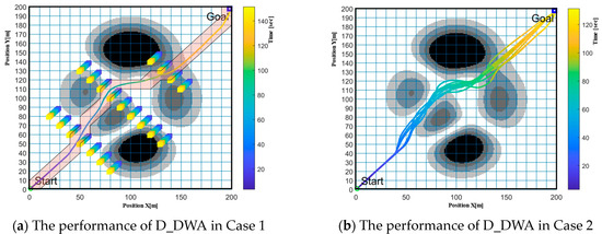
Figure 14.
The performance of D_DWA for planning path in dynamic environment.

Table 8.
Data comparison for the three algorithms in Case 1.

Table 9.
Data comparison for the three algorithms in Case 2.
Based on Figure 12, Figure 13 and Figure 14, it becomes evident that all three algorithms can successfully choose the optimal path while taking into account both risk and length. However, it is worth noting that the I_DWA, due to its absence of global planning guidance, frequently generates longer paths and traverses risk areas, particularly in complex dynamic obstacle environments. The paths generated by the A_DWA are more distorted due to its reliance on local path planning. The global planning algorithm cannot adjust the recommended path in real time, causing the local planner to initiate obstacle avoidance only upon detection. As a result, the robot requires larger turning angles to circumvent moving obstacles, producing a more tortuous and longer path. In contrast, the global planning algorithm of D_DWA can avoid obstacles in advance, reducing reliance on local planning and yielding smoother paths with lower risk and enhanced quality.
Based on the data presented in Table 8 and Table 9, it is clear that the three algorithms perform differently in dynamic obstacle environments, with D_DWA performing best, followed by A_DWA, and then I_DWA. In uniformly dynamic obstacle environments, A_DWA significantly reduces LOP, NORG, and AROG by 17.94%, 34.58%, and 49.19%, respectively, compared to I_DWA. However, A_DWA also increases time cost by 286.68%. In contrast, D_DWA slightly increases LOP by 1.11% compared to A_DWA but reduces NORG, AROG, and Time by 28.57%, 26.60%, and 57.11%, respectively.
In the random dynamic obstacle environment, the path lengths generated by the three algorithms show minimal disparity, while exhibiting significant variations in path risk assessment. A_DWA demonstrates a noticeable improvement in path quality, albeit at the cost of a substantial increase in time consumption. In contrast, D_DWA not only achieves further enhancement in path quality but also effectively reduces time consumption compared to A_DWA. Specifically, when compared to the baseline I_DWA, A_DWA achieves reductions of 12.85% and 14.76% in A_NORG and A_AROG, respectively, while incurring a 257.27% increase in time cost. Conversely, D_DWA achieves reductions of 39.74%, 36.22%, and 63.21% in A_NORG, A_AROG, and A_Time, respectively, compared to A_DWA.
While acknowledging the inherent differences between the global planner algorithms, it is essential to explore the time discrepancies observed between D_DWA and A_DWA. These discrepancies can be attributed to the inherent efficiency differences between the A* and D*Lite algorithms, as well as the application of bi-layer map processing. To investigate how bi-layer map processing enhances time efficiency, this study conducted experiments using the D*Lite algorithm without bi-layer maps in Cases 1 and 2 and recorded the respective time cost. In Case 1, the time cost of D* Lite without bi-layer maps processing was 176.98 s, which is a 40.46% reduction from the 297.26 s recorded with A_DWA’s global planner. After applying bi-layer maps, the time further decreased to 132.64 s, achieving an additional 25.05% reduction. In Case 2, the time cost of D*Lite without bi-layer maps processing was 200.36 s, which was reduced to 116.52 s after application of bi-layer maps processing, representing reductions of 33.13% and 41.84%, respectively. Research findings demonstrate that the application of bi-layer map processing in the D_DWA algorithm effectively enhances its time efficiency.
5.3. Complex Environment
In the dynamic simulation described in Section 5.2, the risk environment was static, lacking dynamic changes. To more effectively evaluate the proposed algorithm’s adaptability to complex environments, this study introduces a more complex simulation experiment. This new experiment features a dynamic risk environment with moving obstacles, significantly enhancing the realism and complexity of the test scenario. Additionally, to comprehensively compare the algorithm’s performance, we included the A_Q algorithm (as described in [28]) in our comparison. The A_Q algorithm combines the A* and Q-learning, and its ability to handle complex environments has been verified in real settings. We use risk level to replace the terrain cost metric used in the original paper and evaluate performance under the same environmental conditions. Note that since the goal is too close to the map boundary, Q-learning will regard it as an obstacle and cannot approach it. Therefore, we set the sgoal = (xgoal, ygoal) = (190–200, 190–200). In the A_Q algorithm, we use red lines to represent the global planning results and colored lines to represent the final planned paths. The other elements in the figure are consistent with Section 5.1.
The dynamic environment includes four distinct risk maps (Risk Maps A to D, as shown in Figure 15). Given the significant time differences between the three algorithms, transitions between these maps are determined by the greater percentage of the x or y coordinates relative to the map’s total length. The specific transition rules are: coordinates less than 15% switch to Risk Map A; those between 15% and 30% switch to Risk Map B; coordinates from 30% to 45% switch to Risk Map C; and coordinates exceeding 45% switch to Risk Map D. Dynamic obstacles are configured exactly as in Case 2. Blue and red pentagrams mark the positions of the agent using the A_DWA and A_Q and the agent using D_DWA, respectively. Furthermore, the starting points, goals, and risk levels are consistent with previous setups. Figure 16, Figure 17, Figure 18, Figure 19 and Figure 20 display the trajectories of the A_DWA, A_Q, and D_DWA algorithms at various stages within this complex environment, while Table 10 details the LOP, NORG, AROG, GT, and Time metrics for the three algorithms.
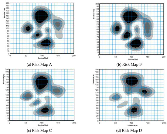
Figure 15.
Four distinct risk maps.

Figure 16.
The performance for the three algorithms in Risk Map A. (a) The performance of A_DWA in Risk Map A. (b) The performance of A_Q in Risk Map A. (c) The performance of D_DWA in Risk Map A.

Figure 17.
The performance for the three algorithms in Risk Map B. (a) The performance of A_DWA in Risk Map B. (b) The performance of A_Q in Risk Map B. (c) The performance of D_DWA in Risk Map B.

Figure 18.
The performance for the three algorithms in Risk Map C. (a) The performance of A_DWA in Risk Map C. (b) The performance of A_Q in Risk Map C. (c) The performance of D_DWA in Risk Map C.

Figure 19.
The performance for the three algorithms in Risk Map D. (a) The performance of A_DWA in Risk Map D. (b) The performance of A_Q in Risk Map D. (c) The performance of D_DWA in Risk Map D.

Figure 20.
The trajectory for the three algorithms in complex environment. (a) The trajectory of A_DWA in complex environment. (b) The trajectory of A_Q in complex envi-ronment. (c) The trajectory of D_DWA in complex environment.

Table 10.
Data comparison for the three algorithms in complex environment.
As illustrated in Figure 16, Figure 17, Figure 18, Figure 19 and Figure 20, all three algorithms successfully reached their goals, yet their performances varied significantly in response to environmental changes. D_DWA and A_Q demonstrated active dynamic adjustment capabilities, whereas A_DWA did not. When the environment changes, A_DWA’s target point imposes greater restrictions on the agent, hindering its ability to navigate complex environments. A_Q can switch to local path planning promptly to manage complex environmental changes, but it is limited to making small adjustments due to its inability to anticipate and plan dodges. D_DWA dynamically adjusts its recommended area using its global algorithm, D*Lite, effectively simplifying the challenges faced by local algorithms. For instance, in Map B, the risk environment is less severe than in Map A. D_DWA alters the recommended area to minimize risk exposure. As the risk level increases from Map B to Map C, and further intensifies from Map C to Map D, D*Lite continues to dynamically adjust its recommended area, consistently decreasing the risk associated with the recommended area and ensuring the final algorithm path is of lower risk.
Table 10 shows that D_DWA is significantly better than A_Q, and A_Q is slightly better than A_DWA. Although the path length planned by D_DWA is 7.43% longer than that used by A_DWA, it achieves reductions of 71.95%, 80.34%, 26.98%, and 35.61% in NORG, AROG, GT, and Time, respectively, when compared to the A_DWA algorithm’s path. This indicates that D_DWA significantly lowers risk despite opting for a slightly longer path. In addition, compared with the A_Q algorithm, it achieves reductions of 1.34%, 67.14%, 78.70%, 34.85%, and 37.63% in LOP, NORG, AROG, GT, and Time, respectively. The superior performance of D_DWA can be attributed to its global algorithm, which dynamically adjusts the recommended area, unlike A_DWA’s global algorithm that does not implement real-time changes. As a result, A_DWA’s local planning algorithm reacts only when encountering risk areas, often missing optimal timing to bypass risk areas. Although the A_Q algorithm can cope with dynamic changes to a certain extent, it is not as effective as D_DWA because it cannot avoid risks in advance. Therefore, the path quality of D_DWA is superior to that of the A_DWA algorithm. The simulation results confirm the effectiveness of the proposed method.
It is worth noting that the change in the color of the lines illustrates the distribution of time consumption. Due to the large number of map nodes, the A_DWA and A_Q algorithms’ global time consumption is concentrated in the initial stage. In contrast, the D_DWA algorithm’s global time consumption is spread throughout the entire process. This distribution improves real-time performance and reduces robot waiting time. Therefore, the D_DWA algorithm has lower time costs and higher real-time efficiency compared to the A_DWA algorithm and A_Q algorithm.
To sum up, in complex environments, the D_DWA algorithm outperforms other compared algorithms in terms of planning speed, path quality, and path flexibility. The global–local coupled path planning framework proposed in this study significantly reduces the consumption of computing resources and enhances robustness by optimizing the fusion method and interactions between coupled algorithms.
Compared with existing global–local coupled path planning algorithms, our research introduces a novel perspective for enhancing efficiency. We focus on optimizing how global and local algorithms are integrated to maximize their respective capabilities. The effectiveness of this method in managing complex environments has been confirmed through simulation comparisons. For robots, applying this method can improve the autonomy and safety of tasks, especially for robots that need to operate in unpredictable environments.
6. Conclusions
To discover the potential of global–local coupling algorithms in enhancing efficiency and path performance in complex environments, this paper proposes a fusion approach that uses the incremental computational capability of the D*Lite algorithm and the local planning capability of DWA. This approach results in significant improvements in algorithmic efficiency and path performance. Furthermore, this paper proposes the concepts of bi-layer map and feasible domains to effectively reduce the number of nodes and constraints during planning, fully harnessing the local planning capability of the DWA algorithm. These improvements guarantee the effectiveness and reliability of the planned paths in the face of complex environments.
In this study, we improve the cost function of D*Lite algorithm and DWA and fuse them to obtain the fusion algorithm for path planning in dynamic and risk environments. This fusion algorithm ensures the generation of the shortest path while minimizing the risk associated with complex environments. We verify the proposed algorithm’s performance across various simulation environments. In the complex environment, compared to the A_DWA algorithm, D_DWA reduces the traversal risk area by 71.95%, cumulative risk by 80.34%, global planning time by 26.98%, and time cost by 35.61%, despite a 7.43% increase in path length. Compared to the A_Q algorithm, D_DWA achieves reductions of 1.34% in path length, 67.14% in traversal risk area, 78.70% in cumulative risk, 34.85% in global planning time, and 37.63% in total time cost.
Some limitations of the current study need to be addressed in future work, including the following:
- (1)
- The current algorithm evaluates all potential costs based on risk. How to materialize risk into multidimensional cost factors in real three-dimensional space has not been fully explored. Future research will explore how to extend this method to the real three-dimensional world to ensure the effectiveness and accuracy of path planning in more complex environments.
- (2)
- The current method assesses risk using the average value of the coarse grid, which may not accurately reflect the actual path’s risk characteristics. Future work will explore customizing the risk assessment method based on specific path planning needs, such as considering the connectivity of the coarse grid or the maximum risk value.
- (3)
- Our algorithm is theoretically practical, but due to the lack of experimental validation with real robots, its effectiveness in real-world situations remains uncertain. In future work, we plan to conduct experimental tests with robots in actual environments to verify and optimize the algorithm’s application effects.
Author Contributions
Conceptualization, Q.H., S.F. and Y.G.; methodology, Y.G., S.F. and Q.H.; software, Y.G. and Z.W.; validation, T.M., J.Y. and Q.H.; formal analysis, T.M.; investigation, Z.W.; resources, Y.G.; data curation, Q.H. and S.F.; writing—original draft preparation, Y.G. and S.F.; writing—review and editing, Z.W., T.M. and Q.H.; visualization, J.Y.; supervision, S.F.; project administration, Y.G.; funding acquisition, Y.G. and J.Y. All authors have read and agreed to the published version of the manuscript.
Funding
This research was funded by the Xi’an Scientific and Technological Projects (23ZDCYJSGG0024-2022, 23ZDCYJSGG0011-2022), the Natural Science Foundation of Shaanxi Province (2019JLP-07, 2019JM-309), the Key Research and Development Program of Shaanxi Province (2024GX-YBXM-530) and the National Key Research and Development Program of China (2021YFB3400502).
Data Availability Statement
Data are contained within the article.
Conflicts of Interest
The authors declare no conflicts of interest.
References
- Wang, N.; Li, X.; Zhang, K.; Wang, J.; Xie, D. A survey on path planning for autonomous ground vehicles in unstructured environments. Machines 2024, 12, 31. [Google Scholar] [CrossRef]
- Cai, K.; Wang, C.; Song, S.; Chen, H.; Meng, M.Q.H. Risk-Aware Path Planning Under Uncertainty in Dynamic Environments. J. Intell. Robot. Syst. 2021, 101, 47. [Google Scholar] [CrossRef]
- Krishnan, J.; Rajeev, U.P.; Jayabalan, J.; Sheela, D.S. Optimal motion planning based on path length minimisation. Robot. Auton. Syst. 2017, 94, 245–263. [Google Scholar] [CrossRef]
- Oral, T.; Polat, F. MOD* Lite: An Incremental Path Planning Algorithm Taking Care of Multiple Objectives. IEEE Trans. Cybern. 2016, 46, 245–257. [Google Scholar] [CrossRef]
- Ataei, M.; Yousefi-Koma, A. Three-dimensional optimal path planning for waypoint guidance of an autonomous underwater vehicle. Robot. Auton. Syst. 2015, 67, 23–32. [Google Scholar] [CrossRef]
- Hart, P.E.; Nilsson, N.J.; Raphael, B. A formal basis for the heuristic determination of minimum cost paths. IEEE Trans. Syst. Sci. Cybern. 1968, 4, 100–107. [Google Scholar] [CrossRef]
- Stentz, A. Optimal and efficient path planning for partially-known environments. In Proceedings of the 1994 IEEE International Conference on Robotics and Automation, San Diego, CA, USA, 8–13 May 1994. [Google Scholar]
- Dijkstra, W. A note on two problems in connexion with graphs. Numer. Math. 1959, 1, 269–271. [Google Scholar] [CrossRef]
- LaValle, S.M. Rapidly-Exploring Random Trees: A New Tool for Path Planning. 1998. Available online: http://lavalle.pl/papers/Lav98c.pdf (accessed on 13 July 2024).
- Kim, P.; Park, J.; Cho, Y.K.; Kang, J. UAV-assisted autonomous mobile robot navigation for as-is 3D data collection and registration in cluttered environments. Autom. Constr. 2019, 106, 102918. [Google Scholar] [CrossRef]
- Tarokh, M. Hybrid intelligent path planning for articulated rovers in rough terrain. Fuzzy Sets Syst. 2008, 159, 2927–2937. [Google Scholar] [CrossRef]
- Li, M.; Sun, Q.; Song, Q.; Wang, Z.; Li, Y. Path Planning of Mobile Robot Based on RRT in Rugged Terrain. In Proceedings of the 2nd International Conference on Computer Science and Application Engineering, New York, NY, USA, 22–24 October 2018. [Google Scholar]
- Carvalho, A.E.; Ferreira, J.F.; Portugal, D. 3D traversability analysis and path planning based on mechanical effort for UGVs in forest environments. Robot. Auton. Syst. 2024, 171, 104560. [Google Scholar] [CrossRef]
- Visca, M.; Powell, R.; Gao, Y.; Fallah, S. Meta-Conv1D Energy-Aware Path Planner for Mobile Robots in Unstructured Terrains. In Proceedings of the 2022 7th International Conference on Robotics and Automation Engineering, Singapore, 18–20 November 2022; pp. 150–157. [Google Scholar]
- Zhang, J.; Zhang, F.; Liu, Z.; Li, Y. Efficient Path Planning Method of USV for Intelligent Target Search. J. Geovis. Spat. Anal. 2019, 3, 13. [Google Scholar] [CrossRef]
- Wang, N.; Xu, H. Dynamics-Constrained Global-Local Hybrid Path Planning of an Autonomous Surface Vehicle. IEEE Trans. Veh. Technol. 2020, 69, 6928–6942. [Google Scholar] [CrossRef]
- Liu, L.; Yao, J.; He, D.; Chen, J.; Huang, J.; Xu, H.; Wang, B.; Guo, J. Global dynamic path planning fusion algorithm combining jump-A* algorithm and dynamic window approach. IEEE Access 2021, 9, 19632–19638. [Google Scholar] [CrossRef]
- Wang, Z.; Li, G.; Ren, J. Dynamic path planning for unmanned surface vehicle in complex offshore areas based on hybrid algorithm. Comput. Commun. 2021, 166, 49–56. [Google Scholar] [CrossRef]
- Jian, Z.; Zhang, S.; Chen, S.; Nan, Z.; Zheng, N. A Global-Local Coupling Two-Stage Path Planning Method for Mobile Robots. IEEE Robot. Autom. Lett. 2021, 6, 5349–5356. [Google Scholar] [CrossRef]
- Song, X.; Gao, S.; Chen, C.B.; Cao, K.; Huang, J. A New Hybrid Method in Global Dynamic Path Planning of Mobile Robot. Int. J. Comput. Commun. Control 2018, 13, 1032–1046. [Google Scholar] [CrossRef]
- Ji, X.; Feng, S.; Han, Q.; Yin, H.; Yu, S. Improvement and Fusion of A* Algorithm and Dynamic Window Approach Considering Complex Environmental Information. Arab. J. Sci. Eng. 2021, 46, 7445–7459. [Google Scholar] [CrossRef]
- Sun, Y.; Zhao, X.; Yu, Y. Research on a random route-planning method based on the fusion of the A* algorithm and dynamic window method. Electronics 2022, 11, 2683. [Google Scholar] [CrossRef]
- Koenig, S.; Likhachev, M. D* lite. In Proceedings of the Eighteenth National Conference on Artificial Intelligence and Fourteenth Conference on Innovative Applications of Artificial Intelligence, Edmonton, AB, Canada, 28 July 2002; pp. 476–483. [Google Scholar]
- Yu, J.; Yang, M.; Zhao, Z.; Wang, X.; Bai, Y.; Wu, J.; Xu, J. Path planning of unmanned surface vessel in an unknown environment based on improved D*Lite algorithm. Ocean. Eng. 2022, 266, 112873. [Google Scholar] [CrossRef]
- Sulaiman, S.; Sudheer, A.P. Modeling of a wheeled humanoid robot and hybrid algorithm-based path planning of wheel base for the dynamic obstacles avoidance. Ind. Robot. 2022, 49, 1058–1076. [Google Scholar] [CrossRef]
- Al-Mutib, K.; AlSulaiman, M.; Emaduddin, M.; Ramdane, H.; Mattar, E. D* Lite Based Real-Time Multi-Agent Path Planning in Dynamic Environments. In Proceedings of the 2011 Third International Conference on Computational Intelligence, Modelling & Simulation, Langkawi, Malaysia, 20–22 September 2011; pp. 170–174. [Google Scholar]
- Yu, J.; Liu, G.; Zhao, Z.; Wang, X.; Xu, J.; Bai, Y. Improved D*Lite algorithm path planning in complex environment. In Proceedings of the 2020 Chinese Automation Congress (CAC), Shanghai, China, 6–8 November 2020; pp. 2226–2230. [Google Scholar]
- Zhang, B.; Li, G.; Zheng, Q.; Bai, X.; Ding, Y.; Khan, A. Path planning for wheeled mobile robot in partially known uneven terrain. Sensors 2022, 22, 5217. [Google Scholar] [CrossRef] [PubMed]
Disclaimer/Publisher’s Note: The statements, opinions and data contained in all publications are solely those of the individual author(s) and contributor(s) and not of MDPI and/or the editor(s). MDPI and/or the editor(s) disclaim responsibility for any injury to people or property resulting from any ideas, methods, instructions or products referred to in the content. |
© 2024 by the authors. Licensee MDPI, Basel, Switzerland. This article is an open access article distributed under the terms and conditions of the Creative Commons Attribution (CC BY) license (https://creativecommons.org/licenses/by/4.0/).