Article

Theoretical and Experimental Investigation of a Novel Wedge-Loading Planetary Traction Drive

1
College of Mechanical and Vehicle Engineering, Chongqing University, Chongqing 400044, China
2
State Key Laboratory of Mechanical Transmissions, Chongqing University, Chongqing 400044, China
*
Author to whom correspondence should be addressed.
Machines 2024, 12(8), 567; https://doi.org/10.3390/machines12080567
Submission received: 27 June 2024 / Revised: 30 July 2024 / Accepted: 10 August 2024 / Published: 19 August 2024
(This article belongs to the Section Machine Design and Theory)

Abstract

:
The development of high-speed motors has stimulated the demand for high-speed reducers. In response to the lack of research on high-speed reducers and the challenge of developing high-speed transmission systems, this study proposes a novel wedge-loading planetary traction drive (WPTD). First, a more accurate theoretical analysis model is established by considering the combined effects of elastic deformation, loading state, and a elastohydrodynamic lubrication (EHL) traction mechanism. Second, the mixed thermal EHL model is introduced into the performance analysis of traction drive for the first time. The fitting formulas for predicting traction contact behavior are derived, and a performance analysis method for all line-contact traction drives is presented. Third, the loading performance, transmission characteristics, and the influence of different parameters on the transmission characteristics of WPTD are analyzed. Finally, the theoretical model is validated by prototype performance tests. The results show that the loading mechanism demonstrates a good self-adaptive loading effect, and WPTD achieves a peak efficiency of 96%. Additionally, WPTD delivers superior efficiency and vibration and noise performance because of its smooth power-transfer characteristics, thereby providing a possible solution for high-speed and low-vibration transmissions.

1. Introduction

The current global environmental issues and electrification trends facilitate the extensive application of motors. Developments in advanced materials, electronic components, and control algorithms continue to push the technical limits of motor speed [1], leading to an increased focus on high-speed motors [2,3]. Compared with conventional motors, drive systems equipped with high-speed motors offer the advantages of power density enhancement, miniaturization, lightweight design, improved efficiency, and cost reduction at equivalent power levels [3,4,5]. With significant reductions in size and weight, compact drive systems offer enhanced design autonomy to numerous applications. However, reducers are usually employed to achieve high output torque with high-speed motors. The trend toward electrification, and the development of new technology in electric motors, have also increased the input speed of reducers, indicating that the design of high-speed drive systems needs to overcome both electrical and mechanical challenges. Compared to high-speed motors, research on corresponding reducers is still scarce, with emerging boundaries and constraints. In addition, high-speed gear transmission systems are subject to severe noise, vibration, harshness (NVH), and scuffing failure [6], which become more prominent with increasing speed. Although improvements can be achieved by increasing manufacture/assembly accuracy, enhancing the surface finish of the gear teeth, adopting coating technology or non-metallic composite materials, and optimizing gear micro-geometry parameters, these methods also lead to higher production costs and difficulties [7,8], resulting in a restricted scope of application. Therefore, developing a reducer with high speed, high efficiency, and low vibration is crucial for fully exploiting the excellent performance of high-speed motors, which has gradually become an important research direction.
In response to the current problems, researchers have investigated a gearless transmission—the traction drive. The traction drive transfers power using traction forces generated by elastohydrodynamic (EHD) fluid film shear stresses between the contact surfaces of moving parts or the friction forces generated by the contact of rough surfaces. The traction drive eliminates the gear-meshing mechanism, fundamentally solving the NVH problem in high-speed gear drive. Due to the special operating principle of the traction drive, it offers several inherent advantages over gears, including zero backlash, high efficiency, low vibration, simple manufacturing, small angular velocity fluctuation rate, and great potential for ultra-high speed. With these features, traction drive is advantageous in high-speed, high-precision, smooth or low-vibration applications, complementing the existing transmission mode. With the continuous development of drive systems in the direction of being high-speed, integrated, and lightweight, the advantages of traction drives can be expected to become more obvious.
Traction drives can be broadly classified into traction-based continuously variable transmissions (T-CVTs) and traction-based fixed ratio transmissions (T-FRTs). Combined with the advantages of the planetary structure and the traction drive, T-FRTs have great potential as a cheaper, quieter, and more attractive solution to the existing problems of high-speed gear transmission, providing a new choice for developing high-speed reducers.
Over the past decades, researchers have focused on structural innovation and prototype testing for T-FRTs. Kim et al. [9] designed a T-FRT with a speed ratio of four for an indoor mobile system. It provided the loading force through the pre-set overload inside the elastic composite ring, making it susceptible to manufacturing accuracy and temperature. Prototype experiments have revealed that the torque capacity decreases with increasing temperature. In addition, since the loading force is independent of the transmitted torque, a sufficiently large loading force must be designed to meet the maximum torque, which reduces the contact fatigue life and is only applicable to low-power transmissions. Therefore, it is necessary to determine and provide an appropriate loading force to achieve the desired functionality of the traction drive and improve performance [10]. The self-adaptive loading overcomes the defects of the above-mentioned loading methods. It automatically adjusts the normal load between moving parts and effectively prevents overloading and slipping, becoming the primary choice for designing T-FRTs. Ai [11,12] proposed a T-FRT with zero spin and self-adaptive loading through conical rollers and a ramp device. It has a speed ratio of 4.6 and a peak efficiency of 99% at an output power of 186.4 kW. The experimental results demonstrate its suitability for high-power applications. Meanwhile, Ai suggested that the zero-spin design minimizes the sliding and reduces the effect of the lubrication conditions on the traction drive. However, the tapered design results in non-parallel axes of the sun roller and planetary rollers, which places higher demands on the design and machining accuracy of the planetary carrier. The introduction of a gyro torque also introduces an instability to high-speed rotation. The cylindrical roller can realize the parallel of the rotation axis and the convenience of processing and assembly, providing an alternative for the zero-spin design. Nevertheless, the internal radial loading problem still needs to be solved. On this basis, Ai et al. [13] proposed another T-FRT design scheme. By setting the sun roller and the ring eccentrically, a convergent gap was formed in the annular space between them. The friction force in the contact area was used to wedge the planetary roller into this gap during operation, thus generating sufficient normal load. The prototype provides a 5:1 reduction ratio for a high-speed motor in an electric oil pump, showing excellent performance at high speeds (12,000 rpm), and with an efficiency of above 97%. Yamanaka et al. [14] applied this structural scheme to the speed-increasing spindle. Due to the high speed and low vibration of the traction drive, the roughness of the milled surface outperformed the commercially available speed-increasing spindle using planetary gears in the cutting test. However, this loading method suffers from two shortcomings: the input shaft needs to be set eccentrically, and the system can only achieve unidirectional rotation, which limits the application scope. By setting a floating lever mechanism, Flugrad and Qamhiyah [15] achieved a coaxial arrangement of T-FRT input and output shafts in this loading method. Despite its advantages, this also increases the complexity of the structure and still has the problem of unidirectional rotation. Wang et al. [16] created a T-FRT for automotive high-speed motors, which overcame the above deficiencies. Prototype test results showed that this T-FRT had satisfactory performance, achieving an efficiency of 96.4% under high-speed and high-torque conditions. Nonetheless, this study focused solely on the experimental design, lacking the necessary theoretical analysis to provide a basis for the subsequent research. Jiang et al. [17,18] proposed a novel T-FRT that achieved self-adaptive loading and a large speed ratio. They also developed a theoretical analysis model and verified the tilting of the planetary rollers during loading, but the resulting spin loss was negligible, with a peak efficiency of 98.5%.
Although some progress has been made in the study of T-FRTs, there are still shortcomings in the following aspects:
  • The advantages of T-FRTs can be enhanced with a large speed ratio, zero spin, and a self-adaptive loading design. However, integrating these aspects into the overall design remains challenging, resulting in a few T-FRTs progressing in the prototype stage and hindering the research and development of T-FRTs;
  • The development of theoretical analysis models for T-FRTs has been hindered by slow progress. Researchers usually simplify calculations by making various assumptions, such as setting the traction coefficient within T-FRTs to a constant value, which neglects the basic elastohydrodynamic lubrication (EHL) traction mechanism, or considering only isothermal EHL contact on the smooth surface, which has only a narrow range of applications. Research on the comprehensive impact of elastic deformation, loading state, surface morphology, thermal effect, and starved lubrication on the traction drive in actual working conditions is still in the early stages;
  • The unique operating principles of traction drives introduce some of the most challenging kinematical and tribological problems for performance prediction [19]. The complex non-linear coupling relationship between macroscopic performance indicators and microscopic contact behavior challenges mathematical modeling and computation, and an effective solution method has not yet been developed.
Based on the above analysis, it is imperative to develop T-FRT to satisfy the new electrification demands and establish a corresponding theoretical model. In order to fill the existing gap, the following work has been carried out in this study:
  • In terms of structural design, this paper proposes a new type of wedge-loading planetary traction drive (WPTD) that can achieve zero spin, large speed ratio, and self-adaptive loading;
  • In terms of theoretical modeling, this paper introduces the mixed thermal EHL model into the performance analysis of traction drive for the first time. In addition, a more refined theoretical analysis model is established according to the structural characteristics of WPTD and the new loading principle. On this basis, the loading performance, transmission characteristics, and the influence of different parameters on the transmission characteristics of WPTD are analyzed;
  • Regarding the solution method, regression analyses based on the results from an extensive set of simulations are performed according to the general operating conditions of the traction drive. On this basis, the fitting formulas for predicting traction contact behavior are derived, considering both hydrodynamic and surface asperity effects, and an efficient and accurate performance analysis method for all line-contact traction drives is presented. These methods significantly facilitate the design and research of subsequent traction drives.
These aspects above have never been discussed in the scientific literature. The objective of this study is to enrich the theoretical design system of traction drive and to provide a valuable addition to this field. WPTD or subsequent improved schemes are expected to satisfy the needs of high-speed motors for high-speed reducers, become a low-cost solution for high-speed drives, and impact electric vehicles, aerospace, high-speed machine tools, medical equipment, and other fields.

2. Model of Traction Drive

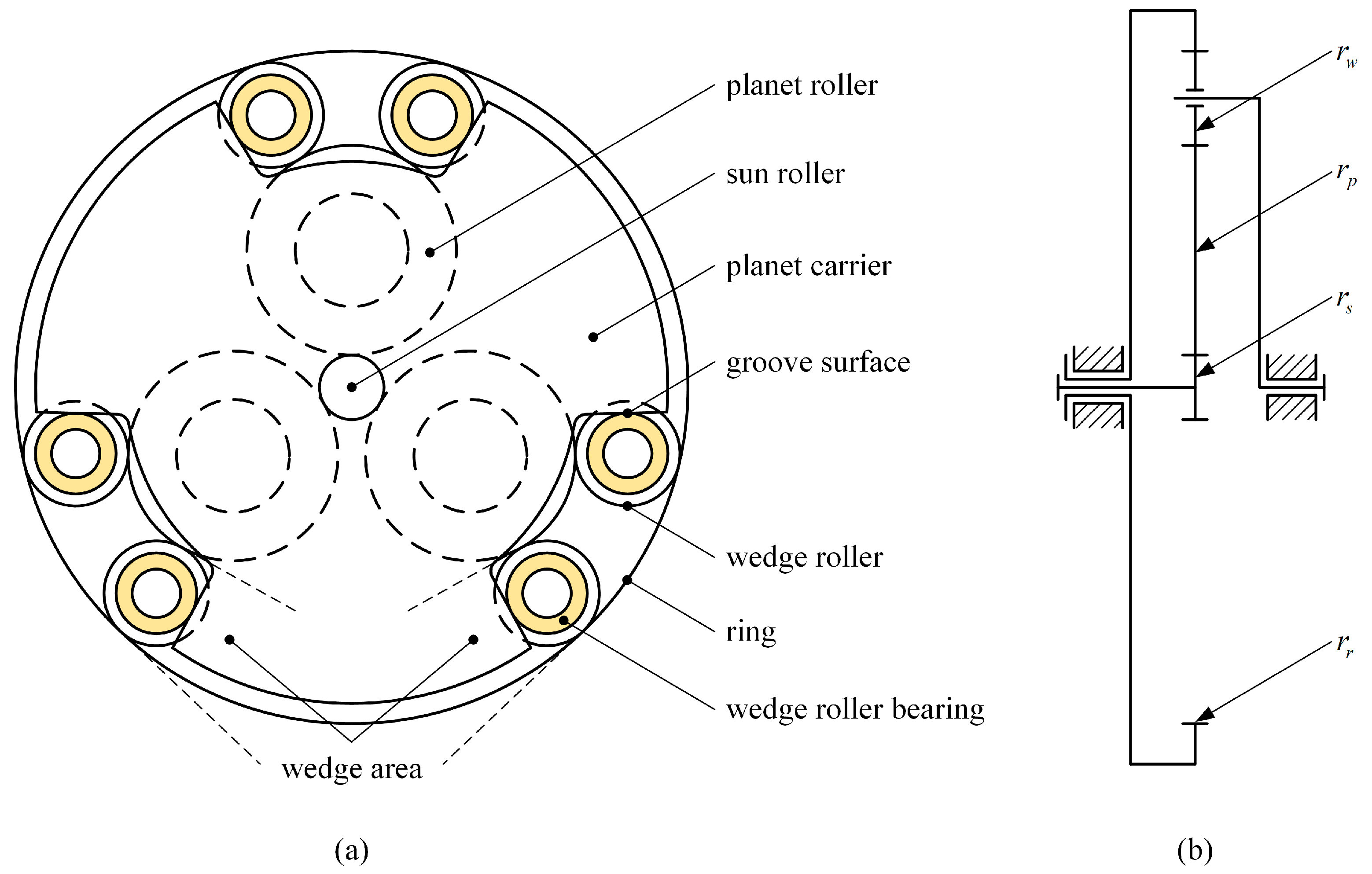
2.1. Structure and Principle

The basic structure of WPTD is shown in Figure 1, including the sun roller, planet roller, wedge roller, ring, and planet carrier. The planet roller is in contact with the sun roller and has a gap in the radial direction with the ring. In this way, a wedge area is formed on both sides of the annular space between the planet roller and the ring. The diameter of wedge rollers is not less than the above gap. The bearing assembled with the wedge roller is not fixed to the planet carrier, but is supported by a carefully designed groove surface on the planet carrier. As a result, the wedge roller is positioned in the wedge area and is in close contact with the planet roller and ring. The planet roller floats freely between the ring and the sun roller, relying on mutual contact with adjacent components to determine the spatial position. This mechanism ensures the dynamic stability of the planetary gear train and minimizes the impact of temperature and manufacturing tolerances. During operation, the power is gradually transmitted through the traction force generated by the contact area of the moving parts. In this case, the combined effect of traction forces on the components and contact forces on the planet carrier groove surface drive the wedge roller into the converging end of the wedge area, effectively wedging it between the planet roller and ring. Consequently, load-related loading forces are automatically generated, ensuring that WPTD generates sufficient traction forces to prevent slippage at high torque and enhance service life.
Table 1 provides a summary regarding WPTD, as well as other T-FRTs in the above literature, comparing them in terms of their structural characteristics and theoretical modeling. It can be seen that the WPTD has the following advantages:
  • The line contact and zero-spin design based on cylindrical rollers minimizes power loss and improves transmission efficiency and loading capacity;
  • The problem of unidirectional rotation when loading with the wedge action is solved by a symmetrical arrangement of the wedge rollers. The coaxial layout of the ring and sun roller is realized, and the design range of speed ratio is expanded;
  • The load acts directly on the wedge roller through the groove surface of the planet carrier, facilitating a more rapid wedging process and enhancing the dynamic response of the system through the superposition of the traction force and the contact force;
  • The floating arrangement of the planet roller requires no additional support for the planet carrier, allowing greater flexibility in designing the planet carrier. Different groove surface designs are available to meet different loading characteristics and performance requirements.
Table 1. Comparison of the WPTD with existing T-FRTs in the literature.
T-FRTsLarge Speed Ratio (≥15)Zero SpinSelf-Adaptive
Loading
Bidirectional
Rotation
EHL Traction
Mechanism
Kim et al. [9]
Ai [11,12]
Ai et al. [13]
Yamanaka et al. [14]
Flugrad et al. [15]
Wang et al. [16]
Jiang et al. [17,18]
WPTD
Symbol ✓: the T-FRT has this characteristic; Symbol ✕: the T-FRT does not have this characteristic.

2.2. Kinematic Analysis

According to the kinematic relationship, the theoretical speed ratios when the ring is fixed at the planet carrier output ScID and when the planet carrier is fixed at the ring output SrID are:
S c I D = 1 r r r s
S r I D = r r r s
where r represents the radius dimension, and the subscripts s, p, w, and r denote the sun roller, planet roller, wedge roller, and the ring, respectively.
It can be seen from Equations (1) and (2), that the theoretical speed ratio is solely determined by the radius of the sun roller and the ring, which has a larger speed ratio at the ring output. Since there is no significant difference between the output methods, the planet carrier output was selected for the subsequent analysis.

2.2.1. Deformation and Displacement

In the actual model, the sun roller, the ring, and the planet carrier are interconnected by bearings and could be consistently regarded as coaxial compared to the floating parts. By restraining wedge rollers, free-floating planet rollers are stabilized and uniformly distributed along the circumference. As the torque increases, a slight displacement of the wedge rollers occurs due to its wedging action, which is absorbed by the floating planet roller. In order to ensure the dynamic stability of the system, it is imperative to consider the effects of the deformation and displacement of each component in detailed designs. For elastic materials, the actual displacement is influenced by structural stiffness and the characteristics of the contact surfaces. Based on the Hertz contact theory, the contact between the parts can be reduced to rigid spring support for examining small incremental movements. The established WPTD continuous deformation model is shown in Figure 2a. Therefore, adjusting the geometric structure during design can alter the contact stiffness and prevent wedge roller penetration into the wedge area, ensuring stable loading of WPTD.
With the circular center of the sun roller as the co-ordinate origin, there is a gradual loss of symmetry along the Z–axis for both the planet roller and wedge roller positions under loading, as shown in Figure 2b. α, β, γ, and φ are the defined characteristic angles. γ is a geometric parameter of the groove surface of the planet carrier, defined as the angle between the contact force of the groove surface and the vertical line of the line connecting the circular centers of the wedge roller and the sun roller. A and B denote the circular centers of the planet roller and wedge roller, respectively. The effective line segment connecting the circular center co-ordinates represents the actual axis distance under loading conditions. Based on the structural characteristics and continuous deformation condition, the following relationship can be obtained:
{ | O A | = r s + r p δ s p | A B l | = r p + r w δ p w - l | A B r | = r p + r w δ p w - r | O A + A B l | δ r w - l = | O A + A B r | δ r w - r = r r r w
where δ is the elastic deformation of the contact area, and the subscripts l and r indicate the left and right sides relative to the planet roller, respectively. Through Equation (3), it is possible to determine the characteristic angles and center co-ordinates that vary with different loads, denoted as α l = O A , O B l , α r = O A , O B r , β l = A B l , O B l , and β r = A B r , O B r . According to the profile equation of the planet carrier groove surface, the normal distance d from the center of the wedge roller to the groove surface can be obtained.

2.2.2. Kinematic Quantities

When transferring tangential load, there is usually a difference in the surface velocity of the contact pair, resulting in fluid film shear stress for traction force transfer. The creep coefficient C represents the relative velocity loss between the active and passive components, serving as the primary reference parameter for characterizing the shear deformation of the lubricant:
C s p = | ω s | r s | ω p | r p | ω s | r s
C p w - l = | ω p | r p | ω w - l | r w | ω p | r p
C p w - r = | ω p | r p | ω w - r | r w | ω p | r p
C r w - l = | ω w - l | r w | ω r | r r | ω w - l | r w
C r w - r = | ω w - r | r w | ω r | r r | ω w - r | r w
where Cjk represents the creep coefficient in the contact region between components j and k; ω represents the angular velocity.
After combining Equations (5)–(8), it can be seen that Cpw-l, Cpw-r, Crw-l, and Crw-r satisfy the following relationship:
( 1 C p w - l ) ( 1 C r w - l ) = ( 1 C p w - r ) ( 1 C r w - r )
A certain degree of creep inevitably leads to deviations between the actual and theoretical speed ratios. Combining Equation (1) and Equations (4)–(9), the actual speed ratio Sc can be obtained as follows:
S c = 1 r r r s ( 1 C s p ) ( 1 C p w ) ( 1 C r w )
In order to characterize the deviation between the theoretical and actual speed ratio, and assess the transmission accuracy of WPTD, a definition of the global sliding coefficient C can be obtained by integrating the creep coefficient of each contact area:
C = ω s / S c I D ω s / S c ω s / S c I D S c I D = ( 1 C ) S c

2.3. Quasi-Static Response

This section investigates the quasi-static response of the WPTD under a specific geometrical configuration. In steady-state conditions, an input torque applied to the sun roller generates an output torque Tout on the planet carrier. The wedging action of the wedge roller guarantees contact forces between transmission parts, which play a crucial role in power transmission.

2.3.1. Loading State Analysis

The loading process can be divided into three stages according to the loading principle. The clockwise rotation of the sun roller is used as an example for analysis, as shown in Figure 3:
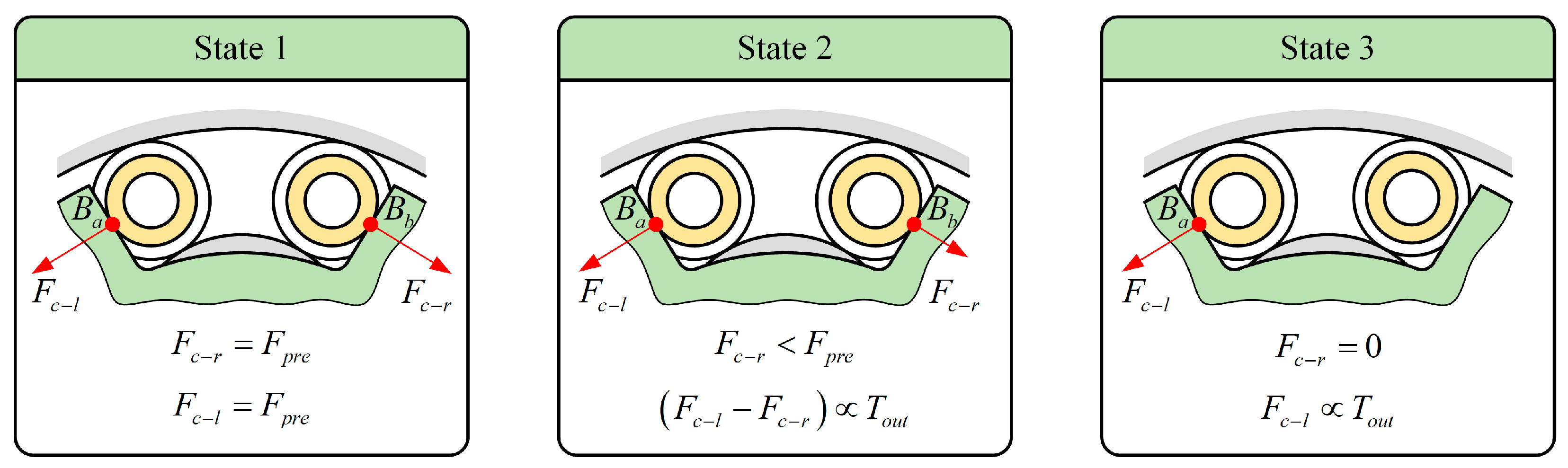
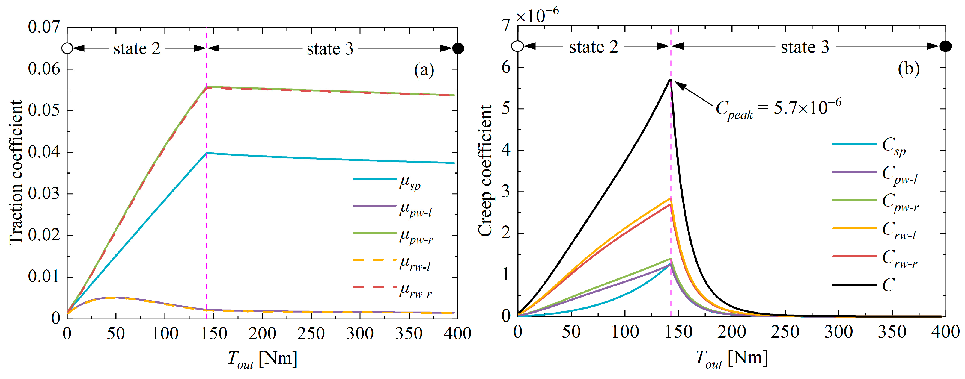
  • In state 1, the centers Bl and Br of the wedge rollers without load remain in their initial positions, and the contact forces Fc-l and Fc-r are equal to the initial preload force Fpre at the contact points Ba and Bb, respectively (see Figure 4);
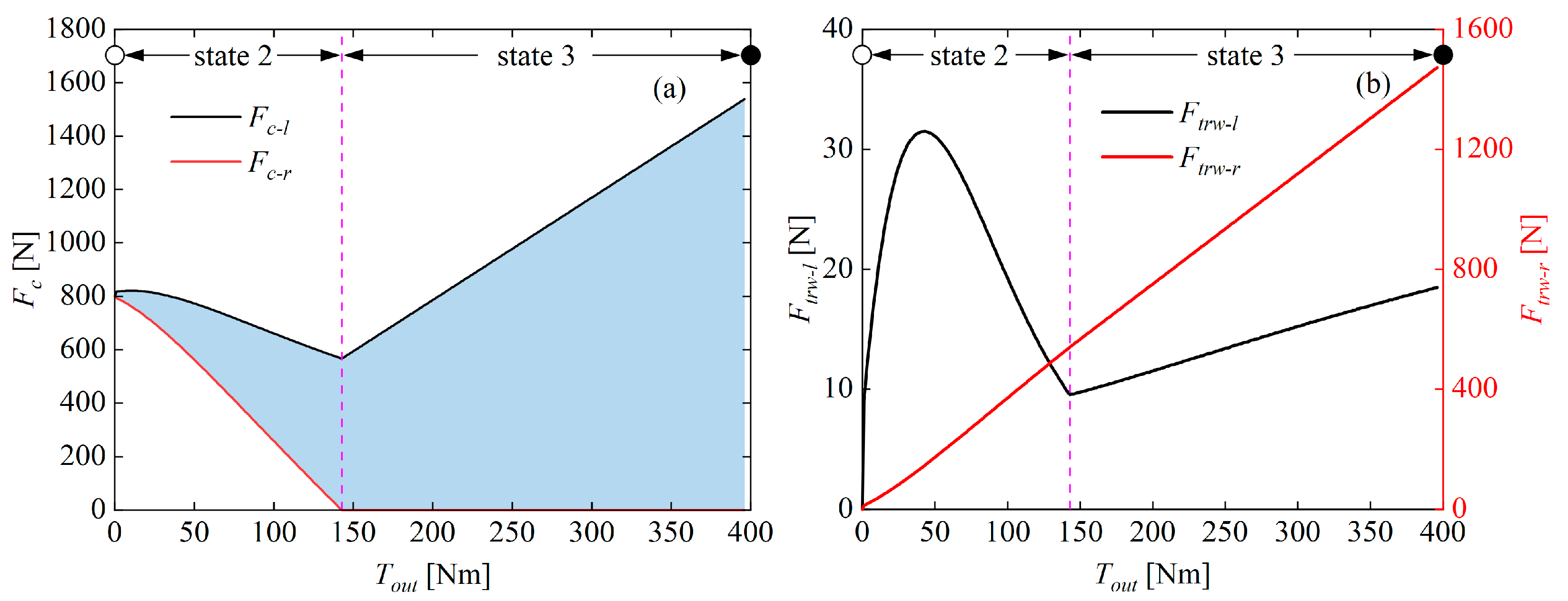
  • In state 2, as the load gradually increases, the right wedge roller undergoes a slight displacement towards the converging end of the wedge area (in the direction away from the planet carrier groove), resulting in a gradual decrease in the contact force Fc-r. The left wedge roller precisely adjusts its position under the joint constraint of the planet roller, ring, and planet carrier to rebalance the system. Consequently, the combined contact forces on both sides of the groove surface provide the output torque Tout;
  • In state 3, the load continues to increase until the point Bb loses contact, Fc-r = 0. The planet roller and wedge roller move together, consistently co-ordinating elastic deformation caused by the load. At this stage, the contact force Fc-l on the groove surface increases with the tangential load and provides the output torque Tout to the WPTD.

2.3.2. Equilibrium Equations

When the WPTD is in stable operation, the force acting on each component is analyzed using the free-body diagram, as shown in Figure 4. In this diagram, F denotes the normal force, Ft denotes the tangential force, and the subscript jk denotes the force between part j and part k.
According to the equilibrium condition, the following relations can be obtained for the left wedge roller:
F p w - l sin β l F c - l cos γ l + F t p w - l cos β l + F t r w - l = 0
F p w - l cos β l F c - l sin γ l F t p w - l sin β l F r w - l + M w ( r r r w ) ( ω s / S c ) 2 = 0
( F t p w - l F t r w - l ) r w 2 T B - l = 0
The equilibrium equation for the right wedge roller is:
F p w - r sin β r F c - r cos γ r F t p w - r cos β r F t r w - r = 0
F p w - r cos β r F c - r sin γ r + F t p w - r sin β r F r w - r + M w ( r r r w ) ( ω s / S c ) 2 = 0
( F t p w - r F t r w - r ) r w 2 T B - r = 0
Similarly, for the free-floating planet roller:
F p w - l sin φ l F p w - r sin φ r + F t p w - l cos φ l + F t p w - r cos φ r + F t s p = 0
F p w - l cos φ l + F p w - r cos φ r F t p w - l sin φ l + F t p w - r sin φ r F s p M p ( r s + r p ) ( ω s / S c ) 2 = 0
F t p w - l + F t p w - r F t s p = 0
where φ = α + β; Mj denotes the mass of the part j; TB denotes the frictional moment generated by the wedge roller bearing.
The planet carrier transmits torque externally through the groove contact force. By considering a specific number of planet rollers N and the output torque is Tout, it can be obtained that:
( F c - l cos γ l F c - r cos γ r ) ( r r r w ) N = T o u t
The support stiffness of the wedge-roller bearing significantly influences the wedge action. It can be seen from Figure 3 that different loading states exhibit distinct force characteristics. The radial displacement of the bearing ring should be harmonized with the internal elastic deformation of the system under the continuous deformation condition (see Figure 2). Therefore, with the clockwise rotation of the sun roller as an example, the following relationship can be established for the contact forces in the grooves:
When d r < ( r B δ c / 2 ) :
{ δ B | F c - l = r B δ c / 2 d l δ B | F c - r = r B δ c / 2 d r
When d r ( r B δ c / 2 ) :
{ F c - l = T o u t / [ ( r r r w ) N cos γ l ] F c - r = 0
where r B is the bearing outside diameter; δ c is the radial internal clearance of the bearing; δ B | F indicates the radial displacement of the bearing ring under the action of radial force F. The details of the method can be accessed in the SKF technical documentation.
Due to the influence of elastic deformation (see Equation (3)), the position of the rollers, characteristic angles, and the loading state vary under different operating conditions, resulting in complex coupling relationships among various variables. Therefore, Equations (12)–(23) can only be explicitly solved by the numerical iterative method.
In addition, the traction coefficient μ j k is defined as the ratio of the tangential and normal forces in the corresponding contact area. The traction coefficient is dependent on the geometry and operating fluid state, necessitating a comprehensive investigation of the contact problem, which will be discussed in Section 3.
μ j k = F t j k F j k

2.4. Efficiency

Transmission efficiency is an essential indicator for evaluating the transmission performance of WPTD. At an input speed of ωs, the relationship between the overall efficiency ηoverall and the output torque Tout can be expressed as:
η o v e r a l l = T o u t ω s T o u t ω s + P l | S c |
where Pl is the overall power loss of WPTD. Benefiting from the zero-spin design, the power loss incurred by rolling contact is free from spin and side slip losses. Therefore, the overall power loss Pl mainly includes the overall sliding loss PlC and the bearing loss PlB.
The overall sliding loss PlC can be expressed as a function of the transmitted power Pjk and the creep coefficient Cjk in each contact area:
P l C = N P j k C j k
It can be seen from Figure 4 that the radial force is only applied to the wedge-roller bearing in a well-assembled WPTD, and the power loss PlB caused by its bearing frictional moment can be calculated by the following equation:
P l B = 2 N ( T B - l | ω w - l | + T B - r | ω w - r | )
The overall efficiency ηoverall can also be obtained from the input power Pin and output power Pout as follows:
η o v e r a l l = | P o u t | P i n = T o u t F t s p r s N | S c |

3. Contact Model

The contact pair in the traction drive plays a vital role in achieving power transfer, with the oil film in the contact area serving as an important medium to generate traction force. In addition, analyzing the traction contact characteristics is a bridge connecting macroscopic transmission performance and microscopic contact mechanism, making it a focal point in the field of traction drive research. Therefore, it is necessary to establish a contact model.

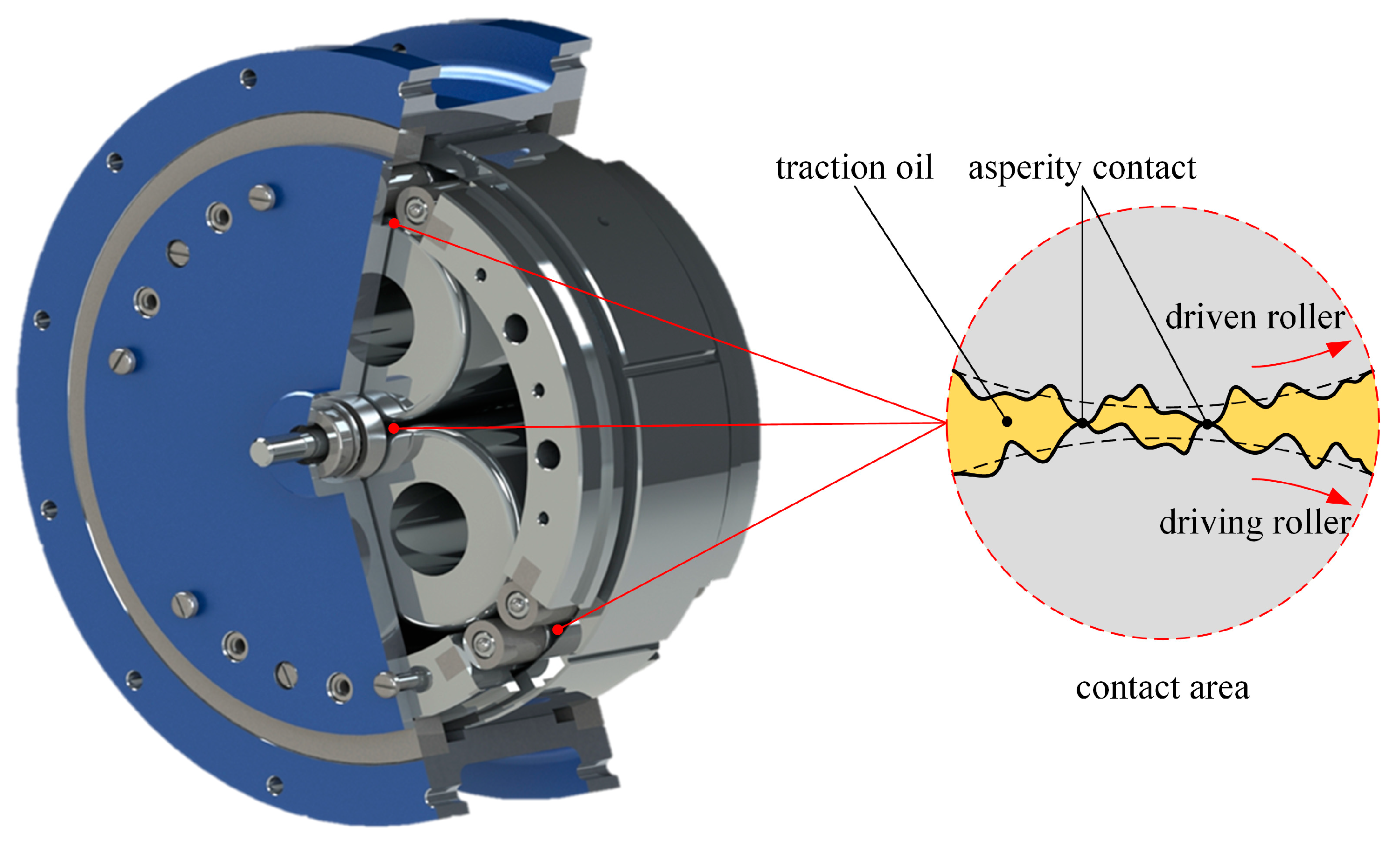
3.1. Mixed Thermal EHL

In order to improve the torque capacity of the traction drive, the contact area is usually designed for operation at high contact stresses (1–3 GPa) and high shear rates [20,21], resulting in a harsh contact environment. Additionally, maintaining a stable oil film in the contact area of the traction drive becomes more challenging under conditions of starved EHL, high temperature, low speed, or overload. Part of the asperity on the actual roller surface penetrates the oil film and they come into contact with each other, thus changing the load balance and complicating the lubrication state, as shown in Figure 5. However, the existing research is based on the assumption of fully flooded smooth surface contact under isothermal conditions, which may introduce significant errors. Mixed EHL is prevalent in traction drives and covers various operating conditions. In this study, the mixed thermal EHL model is employed to describe the behavior of traction contacts using line contact as an example and is extended to the research field of T-FRTs. A more accurate contact model is established, which is also a key step in determining the creep coefficient, traction coefficient, and efficiency. The proposed contact model can fill the gap of the traction mechanism in the theoretical analysis of T-FRTs and improve the prediction accuracy of the theoretical model.
The overall characteristic of mixed EHL represents a combination of coexisting multiple lubrication states, which greatly increases the complexity of modeling. In response to this problem, Johnson et al. [22] introduced the load-sharing concept, where the load is shared between the lubricant and the surface asperities, providing an effective tool for studying mixed EHL. Therefore, the total pressure p at any point is consistently equivalent to the sum of the hydrodynamic pressure p h and the asperity pressure p a :
p = p h + p a

3.1.1. EHL Equations

In a line contact, the hydrodynamic component in Equation (29) can be determined by solving the Reynolds equation, which was modified by Patir and Cheng [23] to incorporate the influence of surface roughness:
x ( ϕ x ρ h 3 12 η p h x ) = u s ( ρ h T ) x
where x denotes the co-ordinate in the moving direction; η is the lubricant viscosity; ρ is the lubricant density; h is the film thickness; us is the rolling speed, which is defined as u s = ( u 1 + u 2 ) / 2 ; u 1 and u 2 are the surface velocities of the driving and driven rollers, respectively. ϕx is the pressure-flow factor in x direction and hT is the average gap between two surfaces [23], which are both functions of the surface roughness σ .
The lubricant viscosity η in the contact area varies with pressure p h and temperature T, and the variation pattern can be described by the Roelands equation [24]:
η η 0 = exp { ( ln η 0 + 9.67 ) [ ( 1 + 5.1 × 10 9 p h ) z ( T 138 T 0 138 ) 1.1 1 ] }
where η0 is the lubricant viscosity at the atmospheric pressure for the initial temperature T0; z denotes the viscosity–pressure index, which is a function of the pressure–viscosity coefficient and η0.
The relationship between lubricant density ρ, pressure p h , and temperature T is determined by the Dowson–Higginson equation [24]:
ρ ρ 0 = 1 + 0.6 p h 1 + 1.7 p h + D ( T T 0 )
where ρ0 is the lubricant density at the atmospheric pressure for the initial temperature T0; D denotes the density–temperature coefficient.
Considering Hertzian geometry and elastic deformation, the lubricant film thickness equation can be expressed as:
h ( x ) = h 0 + x 2 2 R 2 π E x i x e p ln ( x s ) 2 d s
where h0 represents the rigid body displacement; R is the equivalence contact radius; E represents the effective elasticity modulus; xi and xe are the inlet and outlet positions of the lubricant, respectively.
The load-per-unit length w can be obtained by integrating the hydrodynamic pressure p h and asperity pressure p a :
w = x i x e p h ( x ) d x + x i x e p a ( x ) d x
The boundary conditions of the Reynolds equation are defined as:
{ p h = 0 , x = x i p h = 0 ,   d p h d x = 0 , x = x e
The above formula analyzes the traction contact under fully flooded conditions. However, in more realistic situations, high speeds or limited lubricant supply may reduce the lubricant flow rate in the inlet zone, leading to lubricant starvation at the contact [25]. Starved lubrication directly influences the lubrication state, increasing the asperity interactions and accelerating wear [26,27,28,29,30]. In the context of mixed EHL, research on the effect of starved lubrication on traction drives is still scarce at this stage. In view of the lubricant starvation, it is necessary to evaluate the mass flow. The mass flow rate q for line contact can be expressed as [26]:
q l = u s ρ h ρ h 3 12 η p h x
Since the starvation is related to the amount of available lubricant, the starvation degree ζ can be defined as:
ζ = 1 q s q f
where q s and q f denote the mass flow rate in the starved and fully flooded conditions, respectively. ζ = 0 represents the fully flooded condition and ζ = 1 denotes the fully starved condition.

3.1.2. Rough Surface Contact Model

The macro-level contact of ideally smooth surfaces can be adequately described by Hertz contact theory. However, the situation becomes more intricate when the lubricant film fails to completely separate the contact surface, and the asperities start to share part of the load [31]. The asperity pressure can be calculated using the rough surface contact model. Generally, the surface-roughness modeling approaches fall into statistical and deterministic categories. Among them, the statistical approach offers a convenient solution for addressing rough surface contact, thereby facilitating the simulation and prediction of traction contact behavior under different operating conditions [32]. The most commonly used statistical model of rough-surface contact is the GW model proposed by Greenwood and Williamson [33]. In addition, the GW model is solely based on the elastic deformation of the asperities, making it suitable for mildly rough surfaces under light loads. When the surface has increased roughness or under heavy loads, the asperities tend to deform plastically. Chang and Etsion et al. [34] proposed a CEB model that extended the solution to the elastic and full plastic deformation of asperities. Subsequently, Zhao and Maietta et al. [35] extended the analysis to include an elasto-plastic regime and established a ZMC model that considered the elastic, elasto-plastic, and full plastic deformation of the asperities, making it suitable for a wider range of loads and roughness. Beheshti and Khonsari [36] demonstrated the superior accuracy of the ZMC model to the GW and CEB models. Therefore, the ZMC model is considered in this study.
In the ZMC model, the asperity pressure p a can be written as the sum of elastic pressure p e l a s t i c , plastic pressure p p l a s t i c , and elasto-plastic pressure p e l a s t o - p l a s t i c [35]:
p a = p e l a s t i c + p p l a s t i c + p e l a s t o - p l a s t i c = 2 3 E n β 0.5 σ 1.5 σ σ s 2 π h y s h y s + ω 1 ω 1.5 exp [ 0.5 ( σ σ s z ) 2 ] d z + 2 π h d n β σ σ σ s 2 π h y s + ω 2 ω exp [ 0.5 ( σ σ s z ) 2 ] d z + π h d n β σ σ σ s 2 π h y s + ω 1 h y s + ω 2 ω exp [ 0.5 ( σ σ s z ) 2 ] × [ 1 0.6 ln ω 2 ln ω ln ω 2 ln ω 1 ] × [ 1 2 ( ω ω 1 ω 2 ω 1 ) 3 + 3 ( ω ω 1 ω 2 ω 1 ) 2 ] d z
where ω = z h + y s , z represents the height of asperity measured from the mean of asperity heights; y s is the distance from the mean of surface heights to that of asperity heights; the starred variables are normalized by σ . The equivalent surface roughness should be applied to evaluate the contact of two rough surfaces, so σ = σ 1 2 + σ 2 2 . β represents the asperity radius, n is the asperity density, hd denotes the softer material’s Vickers hardness, σ s is the standard deviation of the surface summits, ω 1 is the critical interference at the point of initial yield, and ω 2 is the critical interference at the point of fully plastic flow. In addition, ω serves as a crucial indicator for quantifying the degree of deformation of the micro-asperities. As ω increases, the asperity experiences three different deformation states: when ω ω 1 , the asperity is in an elastic contact state; when ω 1 < ω < ω 2 , elastic and plastic deformation coexist; when ω ω 2 , the asperity is in a plastic deformation state.
According to Equation (38), the asperity pressure can be described as a function of oil film thickness, surface statistical parameters, and material hardness. The calculation method for the above parameters can be found in the literature [24,35,37].

3.1.3. Thermal Analysis

The thermal analysis is essential due to the significant impact of temperature on lubricant viscosity, which in turn affects pressure distribution and traction capacity in the contact area. In the mixed EHL, the primary sources of heat generation are the asperity contact and oil film shear. The heat generated by asperity contact when relative slip occurs on the surface can be expressed as [38]:
Q a = ( u 1 u 2 ) f c p a h
where f c is the asperity friction coefficient, and f c = 0.12 in this study. The change of f c with the surface roughness is ignored.
On this basis, the energy equation considering the roughness effect can be rewritten as:
c p ρ ( u T x u z T z ) = k 2 T z 2 T ρ ρ T ( u p h x ) + η ( u z ) 2 + Q a
where u and u z are the velocities of lubricant along the x and z directions, respectively. c p is the specific heat capacity of lubricant; k represents the thermal conductivity of lubricant.
The temperature distribution along the contact can be obtained from Equation (40), and its boundary conditions are [39]:
{ T ( x , 0 ) = T 0 + k π ρ 1 c 1 k 1 u 1 x T z | x , 0 d s x s T ( x , h ) = T 0 + k π ρ 2 c 2 k 2 u 2 x T z | x , h d s x s
where c 1 and c 2 are the specific heat capacity of the driving and driven rollers, respectively. k 1 and k 2 are the thermal conductivity of the driving and driven rollers, respectively.

3.2. Traction Coefficient

The traction coefficient is usually used to measure the traction force generation ability of the contact pair in traction drives. However, the traction coefficient is not constant, and its contributing factors include lubrication mechanism, contact state, and operating conditions. Accurately calculating the traction coefficient is key to traction drive design and modeling, and the focus of transmission performance analysis. With mixed EHL, the load is shared by the lubricant and the surface asperities. Therefore, the traction force F t is also composed of the shear force F t h generated by the EHD fluid film and the friction force F t a generated by rough surface contact:
F t = F t h + F t a
The rheological model proposed by Bair and Winer is applied to describe the traction oil’s non-linear behavior [40]. The zero-spin design ensures no additional side slip in the line contact area. Therefore, the directions of shear stress and surface creep are the same. The hydrodynamic shear force can be calculated using the integral relation:
F t h = x i x e τ L [ 1 exp ( u s S η h τ L ) ] l d x + x i x e 1 2 h p h x l d x
where S represents the slide-to-roll ratio, S = ( u 1 u 2 ) / u s , and the relationship between S and creep coefficient C is u s S = u 1 C 12 . τ L is the limiting shear stress, τ L = τ 0 + m p h , τ 0 is the Eyring characteristic stress, m is the limiting shear stress coefficient, and l is the contact length.
According to the Coulomb friction model, the friction force in the asperity contact area is directly proportional to the asperity load [41,42], which can be written as:
F t a = x i x e f c p a l d x = f c F ( L a 100 )
where F denotes the total normal load and La is the asperity load ratio, defined as [24]:
L a = x i x e p a ( x ) d x x i x e p h ( x ) d x + x i x e p a ( x ) d x × 100 %
Finally, the traction coefficient μ is obtained by combining Equation (24) and Equations (42)–(45):
μ = f c ( L a 100 ) + 1 w x i x e τ L [ 1 exp ( u s S η h τ L ) ] + h 2 p h x d x

3.3. Numerical Simulation and Formula Fitting

The research on traction contact under mixed thermal EHL places high requirements on the numerical solution algorithm for the following reasons:
  • The traction contact area is usually under high contact stresses and high shear rates which could lead to poor convergence in the numerical calculation;
  • The typically large viscosity–pressure coefficient of the traction oil allows it to form a high-viscosity oil film under heavy loads but also causes the lubricant viscosity to be extremely sensitive to pressure variations, which is detrimental to the stability of numerical iterations;
  • The mutual coupling of factors such as surface roughness, thermal effect, starvation, and extreme working conditions is another source of instability and significantly increases the difficulty of numerical calculations.
In this study, the above equations are rewritten into dimensionless forms and discretized using the finite difference method. The convergence and accuracy are ensured by refining the mesh. In addition, the convergence is evaluated based on the total load error, temperature distribution error, and relative error of two iterations of the pressure distribution. The iteration process continues until the error falls below a specified tolerance value (1 × 10⁻⁴). The final results include pressure, film thickness, temperature distribution, and traction oil characteristics. Based on these results, the asperity load ratio and traction coefficient are determined.
Furthermore, the unique operating principle of traction drives presents some of the most challenging kinematical and tribological problems for performance prediction. The theoretical models of traction drives include kinematic, mechanical, and contact models. The operation and lubrication conditions of each contact area differ, and the force, deformation, and motion must be co-ordinated simultaneously in the system, causing the parameters to couple with each other [17]. Direct application of the mixed thermal EHL model requires lots of numerical iterations to simulate its characteristics, resulting in excessively long computations. It is vital to seek an accurate and efficient method.
Therefore, this section establishes fitting formulas for the engineering calculation using various dimensionless parameters, including dimensionless film thickness, speed, load, material, surface roughness, thermal effect, and hardness:
H = h R ,   U = η 0 u s E R ,   W = w E R ,   G = α 0 E ,   σ ¯ = σ R ,   K = E R k η 0 T 0 ,   V = h d E
According to the general operating conditions of traction drives, the ranges of input parameters for the numerical simulation are presented in Table 2. A typical commercial traction oil, Santotrac 50, is selected, whose fluid properties are shown in Table 3.
In order to improve the fitting accuracy, over 30,000 different operating conditions are numerically calculated based on the theory in Section 3.1 and the ranges of inputs in Table 2. Moreover, regression analyses are performed on the numerical results to fit the formulas for predicting the minimum film thickness hmin, central film thickness hc, asperity load ratio La, and traction coefficient μ. Then, the starvation degree ζ is introduced to modify these formulas. Finally, the fitting results are as follows:
H min = h min R = ( 1 0 . 8081 ζ 1.0458 ) × 0.6284 W 0.0867 U 0.6504 G 0.6015 × ( 0.1984 σ ¯ 0.6885 V 0.0395 W 0.0789 U 0 . 48 G 0.5097 K ¯ 0.267 0.195 S 0.175 + 1 )
H c = h c R = ( 1 0 . 9834 ζ ) × 0.6279 W 0.0854 U 0.6431 G 0.5987 × ( 0.0685 σ ¯ 0.7423 V 0.1019 W 0.168 U 0 . 5613 G 0.6622 K ¯ 0.509 + 0.0758 S 0.1058 + 1 )
L a = 0.2097 W 0.4542 U 0.0526 G 0.0367 × { ln [ 1 + ( 1 0.672 ζ ) 11.8629 × ( 0.9149 σ ¯ 7.3373 V 0.0271 W 0 . 4059 U 4.6342 G 3.5814 K ¯ 0.6862 + 0.2591 S 0.5283 ) ] }
μ = f c × L a 100 + 0.0139 × 1 exp { 2.8774 S 0.3235 × [ 2.3393 + ( 1 + 0.8774 ζ 0.6828 ) × ( 1 L a / 100 ) 9.3525 × W ¯ 2.9209 U ¯ 0.0593 K ¯ 0.589 ] } × ( 1 L a 100 ) ÷ ( W ¯ 4.8 K ¯ 2 S 0.5125 × s i g n ( S ) + 0.1503 )
where W ¯ = W / ( 3.2 × 10 5 ) , U ¯ = U / ( 3 × 10 12 ) , and K ¯ = K / ( 1.3 × 10 9 ) . s i g n ( x ) is the sign function, defined by s i g n ( x ) = 1 for x > 0 and s i g n ( x ) = 1 for x < 0 .
It should be noted that Equations (48)–(51) are fitting formulas based on the simulations of a specific lubricant (Santotrac 50) and a specific surface material (steel), where all design requirements for line-contact traction drives are met. Equations (48) and (49) can be used to evaluate the lubrication state. Equation (51) provides a new, practical, and fast traction coefficient calculation method. It comprises the asperity friction (first term) and the hydrodynamic shear (second term). The film thickness error is defined as | H s H f | / H s , the asperity load ratio error is defined as | L a s L a f | , and the traction coefficient error is defined as | μ s μ f | . Subscripts s and f denote the corresponding simulation values and fitting values, respectively. The results show that the maximum errors of H min , H c , L a , and μ are 7.1893%, 4.6103%, 4.7630%, and 0.0151, respectively, while the mean errors are 1.3565%, 0.8941%, 0.3837%, and 0.0038, respectively. In addition, the fitting errors under starvation conditions ( ζ 0 ) are slightly greater than those under fully flooded conditions ( ζ = 0 ), but the results are still acceptable. Table A1 (Appendix A) presents part of the results derived from the simulations and the fitting formulas, along with their corresponding errors, indicating that the fitted and simulated values are very close and can meet the requirements for engineering applications.

4. Results and Discussions

Based on the working principle of the new wedge-loading mechanism, this study derives and develops a theoretical analysis model considering the combined effects of elastic deformation, loading state, and mixed thermal EHL, which can be used for design optimization, performance analysis, and dynamic simulation. The ultimate torque of current T-CVTs is about 400 Nm [43]. Therefore, the torque capacity is used as the design target of WPTD, and the specific geometric parameters are listed in Table 4. This section takes the clockwise rotation of the sun roller as an example for analysis, as the counter-clockwise rotation yields relatively symmetric laws and characteristics, which are not worth repeating. Moreover, modern bearing steels can operate at contact stresses of up to 4 GPa [13,44]. To ensure adequate safety factors of WPTD under a wide range of operating conditions, this study specifies a maximum contact stress of 2 GPa for line contacts and does not consider material property variations. In order to effectively balance model complexity and computational efficiency, the fitting formulas proposed in Section 3 are used to link the macroscopic performance and the microscopic contact behavior. The specific calculation process is shown in Figure 6. Based on the calculated results, the performance of WPTD is evaluated, and the influence of different parameters on transmission performance is analyzed.

4.1. Performance Analysis

The displacement of the circular center of wedge rollers along the x direction under different output torques is shown in Figure 7, where xw-l is the displacement of the left wedge roller, and xw-r is the displacement of the right wedge roller. In state 2, as Tout increases, the wedge rollers move away from the groove surface of the planet carrier and the displacement of the right wedge roller is greater than that of the left wedge roller, causing the contact force Fc to gradually decrease and Fc-r < Fc-l (Figure 8a). In state 3, the bearing of the right wedge roller is out of contact with the planet carrier groove. The left wedge roller begins to move in the opposite direction under the joint constraint of the planet roller, ring, and planet carrier to rebalance the system. At this point, Fc-r = 0 and Fc-l gradually increase. Therefore, it can be seen that the variation of wedge roller positions is closely related to the loading state and the contact force.
Figure 8 shows the variation of the contact force Fc at the groove surface of the planet carrier, and the tangential force Ftrw at the ring with the output torque Tout. The contact force on both sides of the groove surface in the initial state equals the initial preload force. As Tout increases, the right wedge roller moves toward the converging end of the wedge area (away from the groove surface of the planet carrier), causing Fc-r to gradually decrease and the difference between Fc-l and Fc-r (the blue area in Figure 8a) to gradually increase. According to Equation (21), the difference is proportional to Tout. When reaching a certain load, F c - r = 0 , state 2 shifts to state 3, and the slopes of the corresponding Fc-l and Ftrw-l curves undergo step changes. The reason is that the loading state changes the force characteristics inside WPTD (Figure 3), bringing the system back into equilibrium. Also shown in Figure 8, the tendency of the right wedge roller to enter the wedge area allows the system to generate sufficient loading forces, thereby producing greater traction forces. Therefore, the power is mainly transferred from the contact area on the right side, and the tangential force acting on the right wedge roller is much greater than that on the left side. In state 3, Fc-l increases with the increasing Tout, and the tendency of the left wedge roller to move away from the wedge area acts on the planet carrier through the groove surface and outputs torque externally.
The traction coefficient is fundamental in the design and modeling of traction drives, and a key indicator to measure the performance of the loading mechanism. Figure 9a depicts the relationship between the traction coefficient μ and the output torque Tout. As Tout increases, μ increases from 0. The loading mechanism in state 3 causes the traction coefficient of each contact area to stabilize by adjusting the normal load, showing a good loading effect. Since the power is mainly transmitted from the right side, μpw-r and μrw-r are greater than μpw-l and μrw-l, but the magnitudes of the traction coefficient are small (within 0.06). This result confirms that the proposed loading mechanism can ensure that WPTD always operates in the linear region of the traction curve, thus avoiding destructive slippage under ultimate load while providing an adequate safety factor.
The creep coefficient reflects the speed loss, which has important engineering significance in traction drives. Figure 9b shows that, as Tout increases, the creep coefficient increases in state 2, decreases in state 3, and gradually stabilizes. The loading state determines the trend of the creep coefficient because the normal load in each contact area in state 2 is mainly provided by the preload force. The traction coefficient increases under a higher load (see Figure 9a), consequently increasing the creep coefficient. In contrast, the loading mechanism in state 3 can automatically adjust the normal load to an appropriate value due to the wedge action, which effectively reduces the creep coefficient. The global sliding coefficient C shows a similar variation pattern to the creep coefficient of each contact area, and its maximum value Cpeak appears at the wave peak, which is also the demarcation point for loading state changes. At n s = 10,000   rpm and F p r e = 800   N , C p e a k = 5.7 × 10 6 , which is much lower than 1%. It is confirmed that the loading mechanism produces the optimal loading force and effectively reduces the sliding. In addition, Cpeak can reflect the sliding level of WPTD over the entire load range and is an important performance parameter that provides an objective function for subsequent design optimization.
Figure 10 shows the curves of the overall efficiency ηoverall calculated with Equations (25) and (28) at different input speeds ns. As Tout increases, ηoverall first increases and then levels off. This trend is in line with the experimental results in [13]. The loading mechanism effectively avoids the significant reduction in ηoverall under heavy loads, thus improving the torque capacity of WPTD. Under low torque conditions, the efficiency depends heavily on the load. At this point, the system is overloaded under the preload force, and the friction loss in bearings and seals accounts for a large proportion of the transmitted power, leading to a lower efficiency. Under high torque conditions, the influence of internal resistance becomes smaller, and the efficiency is improved, with a maximum efficiency of 98.7%. Moreover, ηoverall decreases slightly with increasing ns and is more pronounced at low loads, consistent with the experimental results in [12,13]. The reason for this result is that creep coefficients are reduced at high speeds (see Figure 11a), while the power loss Pl is still increased. Under high loads, the increased power losses become insignificant compared to the power delivered. At this point, the efficiency is high and almost independent of speed. Moreover, the two efficiency calculation methods (Equations (25) and (28)) yield the same results, validating the model.
The above analysis reveals that the speed slightly affects the transmission efficiency, demonstrating the excellent high-speed transmission performance of WPTD.

4.2. Parameter Effects

The theoretical analysis model derived from this study provides the opportunity to clarify the effects of different parameters on transmission performance. Since the peak global sliding coefficient Cpeak can reflect the transmission accuracy, efficiency, and loading performance of WPTD, the variation of Cpeak with each parameter is compared and analyzed. Other parameters are kept constant during the analysis. Highlighting certain trends and patterns could guide the design process of subsequent T-FRTs.
Figure 11 shows the variations of Cpeak under different input speeds, preload forces, surface roughness, starvation degrees, characteristic angles, and contact lengths. As shown in Figure 11a, a higher input speed ns yields a smaller global sliding coefficient peak Cpeak. For example, C p e a k = 6.2 × 10 6 when n s = 2000   rpm , and C p e a k = 5.7 × 10 6 when n s = 10,000   rpm . This result is because the asperity load ratio La decreases with the increase of ns, and the tangential force in WPTD is mainly provided by the shear stress of the fluid film. At this point, Cpeak is closer to the results under the smooth surface assumption. Furthermore, the temperature rise in the contact area due to high speed can be ignored under zero spin and low sliding [45], and the increased shear rate effect dominates, thus achieving higher traction force at lower sliding.
The Influence of Initial preload force Fpre on Cpeak is shown in Figure 11b. As Fpre increases, the load threshold in state 3 increases. Thus, a larger torque is required to disengage the right groove surface of the planet carrier from contact with the bearing, thereby reducing Cpeak. Moreover, Cpeak is smaller under a large Fpre. For example, at F p r e = 500   N , C p e a k = 4.8 × 10 4 , and a large sliding occurs due to insufficient preload force. At F p r e = 1000   N , C p e a k = 6.9 × 10 7 . The sliding of WPTD can be adjusted by altering the initial preload force. Nevertheless, when F p r e 800   N , increasing the preload force does not contribute much to improving sliding. In other words, at this time, reducing Cpeak at the cost of increasing the contact force would become an unreasonable solution. Additionally, an excessive preload force can even reduce contact fatigue life and transmission efficiency [10,12,46]. Therefore, choosing an appropriate preload force can effectively reduce sliding and improve efficiency and power density.
Surface roughness and starvation are key factors affecting oil-film formation and lubrication state. As shown in Figure 11c,d, Cpeak also varies with surface roughness σ and starvation degree ζ . On actual rough surfaces, the contact pair cannot be completely separated by the fluid film, and the load is shared by the lubricant and the surface asperities. The asperity load ratio La increases as σ and ζ increase, causing the surface asperities to carry more load. Although friction drives can minimize sliding and increase the maximum traction coefficient, the reduced normal load on the fluid film also reduces the lubricant viscosity in the contact area, thus increasing sliding. These two completely opposite effects must be considered together. It should also be noted that the asperity contact exacerbates the surface wear of rotating components and reduces the torque capacity of the device. Therefore, a transmission-component surface that is as smooth as possible is usually desirable for achieving the film parameter Λ = h min / σ > 3 . As shown in Figure 11c, the effect of surface roughness on Cpeak is negligible when σ 0.1   μ m . Considering the actual processing conditions, the roughness of the roller can be set to 0.1 μm to improve contact conditions as much as possible. Furthermore, starvation has a greater impact on Cpeak, which deserves due attention in the traction-drive design process.
The groove surface design of the planet carrier directly affects the wedging process by changing the force characteristics of the wedge roller, thus affecting the loading characteristics and performance. Figure 11e depicts the Cpeak, corresponding to different characteristic angles γ of the groove surface. Among them, γ is positive when in the same direction as defined, and negative otherwise (Figure 2b). It can be observed that γ affects Cpeak. γ can achieve a low Cpeak within a limited range of angles ( 10 γ 10 ), and an excessively large or excessively small value will sharply increase sliding.
Since the contribution of the creep coefficients Crw-l and Crw-r to the global sliding coefficient C is the largest (Figure 9b), optimizing the contact between the wedge roller and the ring can effectively improve WPTD performance. Crw-l and Crw-r can be altered by adjusting the contact length lrw between the ring and the wedge roller, thus affecting Cpeak. The specific relationship is shown in Figure 11f. As lrw increases, the contact stress between the wedge roller and the ring decreases, but Cpeak gradually shifts to the right, and the load threshold in state 3 increases. These effects, together, lead to a gradual decrease in Cpeak. It is noteworthy that the torque capacity of WPTD increases with an increase in lrw, and when l r w 26   mm , lrw is independent of the torque capacity. At this point, the weakest link in the system changes from the contact between the ring and the wedge roller to the contact between the planet roller and the wedge roller. Therefore, a properly designed lrw can reduce sliding while keeping the torque capacity unchanged.
According to the above analysis, the preload force, characteristic angle, and contact length exhibit the most significant effects on the global sliding coefficient. Therefore, these parameters deserve special attention during design to avoid transmission failure due to excessive slippage. Moreover, they should be properly adjusted based on the application scenario to balance the global sliding coefficient and torque capacity.

5. Experimental Verification

In order to validate the theoretical model and WPTD performance, an experimental study on a prototype is essential. Before the transmission performance test, a white light interferometer was used in this section to detect the surface roughness of the prototype transmission components, providing necessary input parameters for theoretical calculations. The sun roller, planet roller, wedge roller, and ring were manufactured from bearing steel. Their surfaces were hardened to over 60 HRC, and ground and polished to within 0.1 μm. Figure 12a shows the main transmission components of WPTD and their surface inspection results. Figure 12b illustrates the general view of the WPTD prototype with the end cap removed.

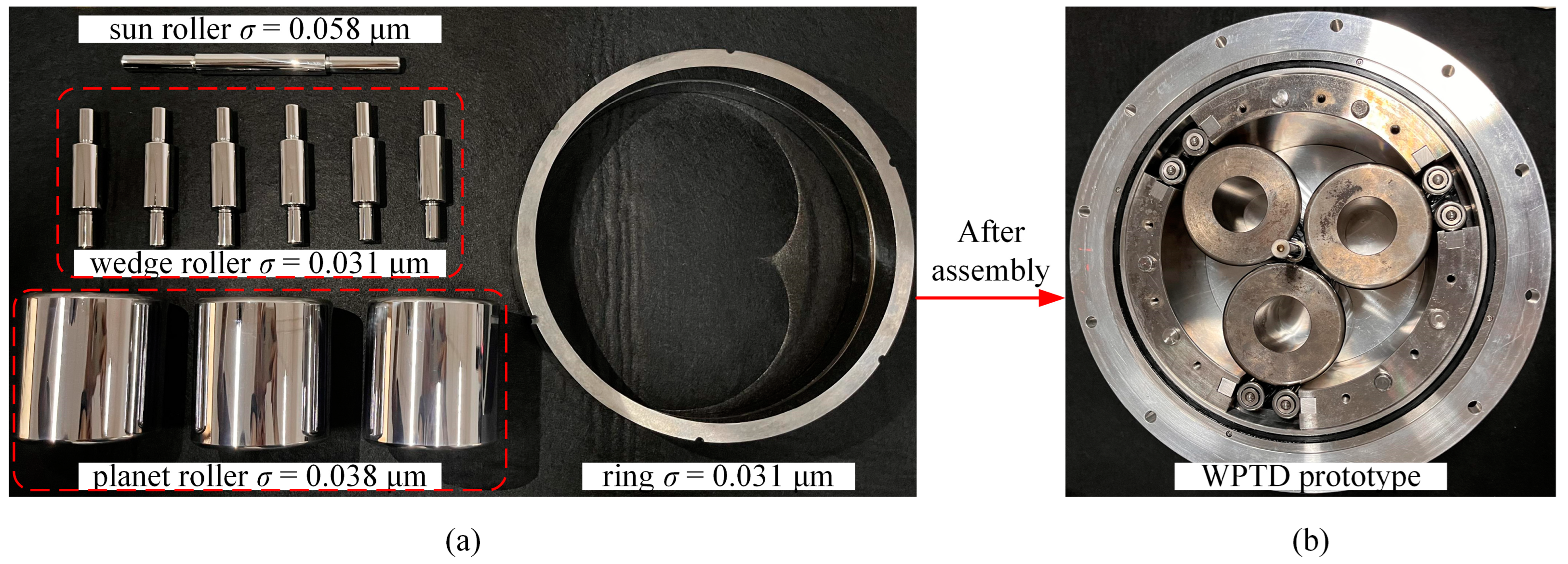
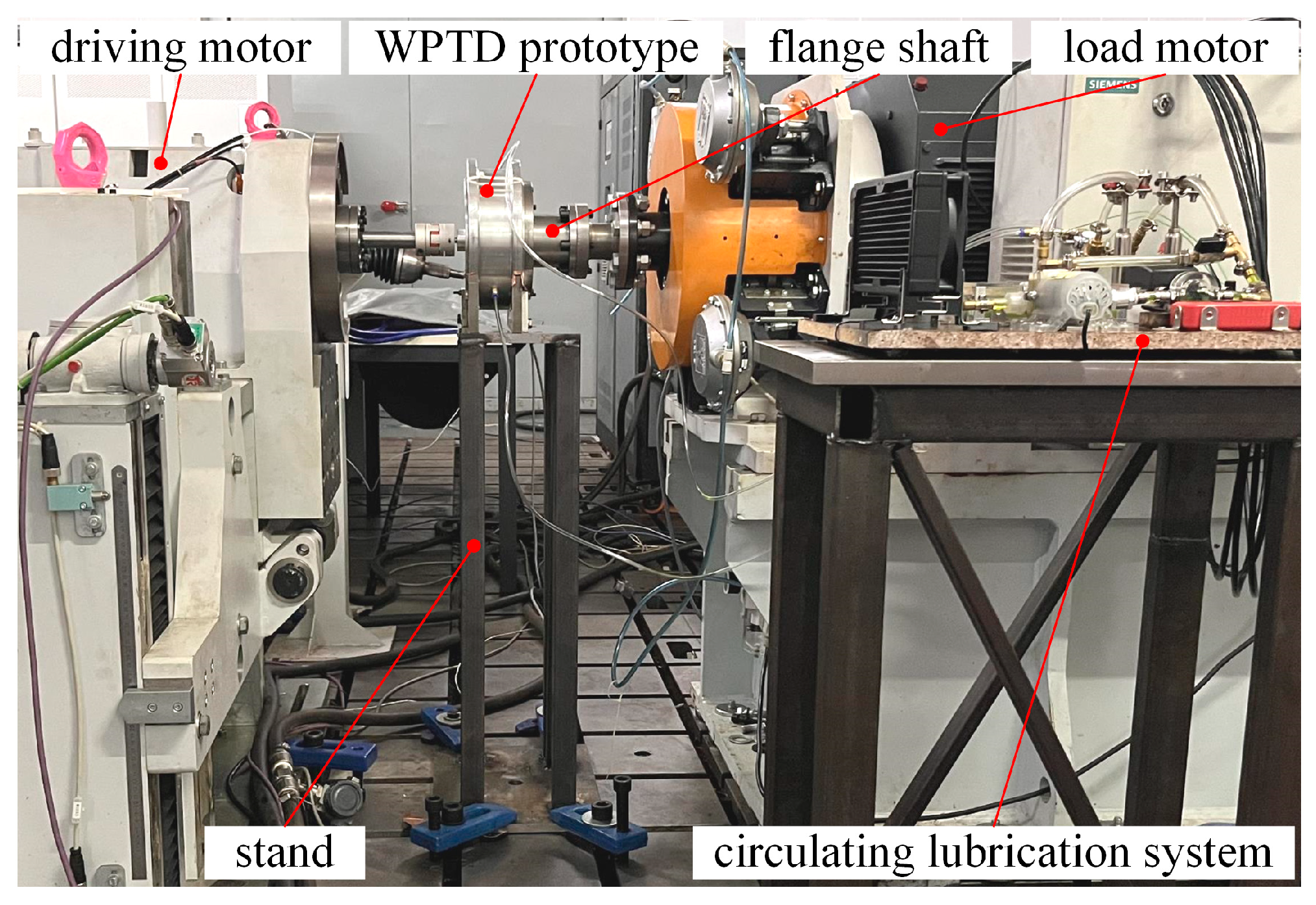
5.1. Test Rig Assembly

The test was undertaken at a specialized automotive test facility. Figure 13 shows the test rig and the WPTD prototype. The input shaft of the test rig integrates a driving motor (max speed 9000 rpm), an input encoder, and an input torque sensor (error below ±0.05%), while the output shaft of the test rig includes a load motor (rated torque 3701 Nm), an output encoder, and an output torque sensor (error below ±0.05%). The prototype was mounted on the stand with the sun roller connected to the input shaft and the planet carrier connected to the output shaft through a flange shaft. The ring mounted on the prototype housing was fixed to the stand. The shafts and the prototype were co-axially aligned within a tolerance of 0.01 mm using a laser alignment instrument. A circulating lubrication system provided lubricant (Santotrac 50) to the traction contacts.

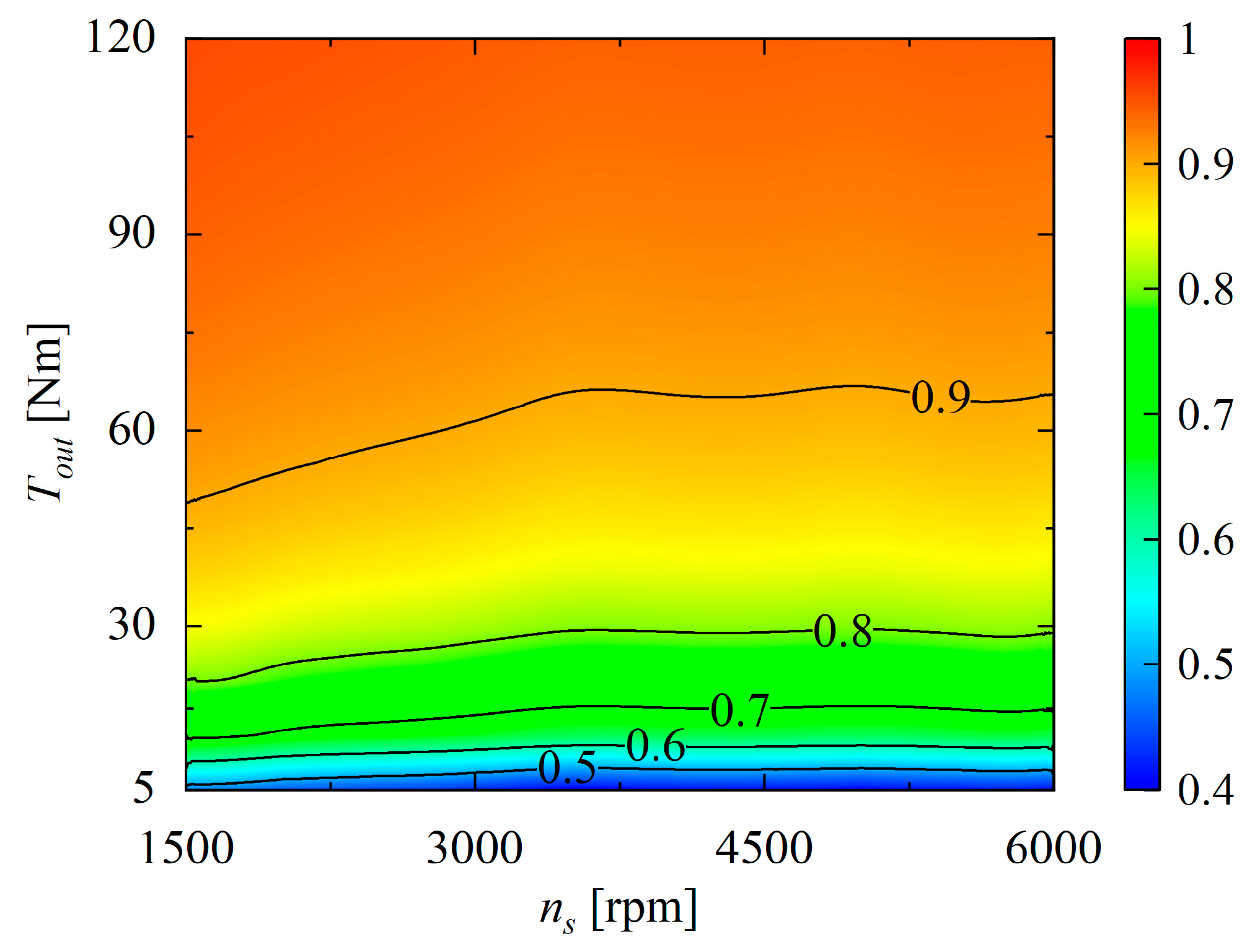
5.2. Efficiency Test

Efficiency involves the transfer and utilization of energy, which can comprehensively reflect the velocity loss caused by micro slip and the torque loss caused by macro friction. It is one of the key performance parameters of the traction drive, and the final result of the theoretical analysis. Therefore, an efficiency test on the prototype can directly validate the theoretical model proposed in this paper. Figure 10 shows that as Tout increases, the efficiency ηoverall first increases sharply (when T o u t 120   Nm ), and then it tends to level off (when T o u t > 120   Nm ). At this point, ηoverall is independent of ns and Tout. The efficiency of the prototype within 120 Nm offers more reference values, and the testing cost can be effectively reduced.
A series of prototype tests were conducted to evaluate transmission efficiencies under application conditions. The control system of the test rig was programmed to implement the desired variations in input speed ns and output torque Tout by controlling the driving motor and load motor. The prototype was tested at a steady input speed under well-lubricated conditions while the output torque was increased from 10 Nm to 120 Nm in a 10 Nm step. Meanwhile, the data acquisition system of the test rig recorded the readings of the encoders and torque sensors on the input and output sides, and the input power Pin and output power Pout were calculated. Thus, the measured efficiency of the prototype was obtained based on Equation (28). Subsequently, the process was repeated, with the torque dropped to the initial level and the input speed set to the next level.
Figure 14 compares the theoretical and experimental results of the overall efficiency at different input speeds. The measured efficiency is slightly lower than the theoretical efficiency, and the transmission efficiency error is defined as the difference between the theoretical and experimental results. The empirical formula provided by SKF is used to calculate the bearing friction moment in this study, and it reduces the calculation accuracy of the theoretical model to a certain extent. Under low torque conditions, the friction loss in bearings accounts for a large proportion of the transmitted power, thus leading to a larger error. In addition, the churning losses caused by high-speed conditions may also introduce additional errors. It can be seen that the maximum error is below 9%. The efficiency of WPTD derived from theoretical calculations agrees with the experimental results in terms of magnitude and variation trend, validating the theoretical model and the proposed numerical method. Moreover, the peak efficiency ηpeak seemed to decrease slightly as ns increased (Figure 14f), finally stabilizing in the range of 93–94%.
Figure 15 shows the measured efficiency map of the WPTD prototype, where the efficiency increases with Tout but is almost independent of ns, basically consistent with the results in Figure 10. In summary, the theoretical analysis model has sufficient prediction accuracy.

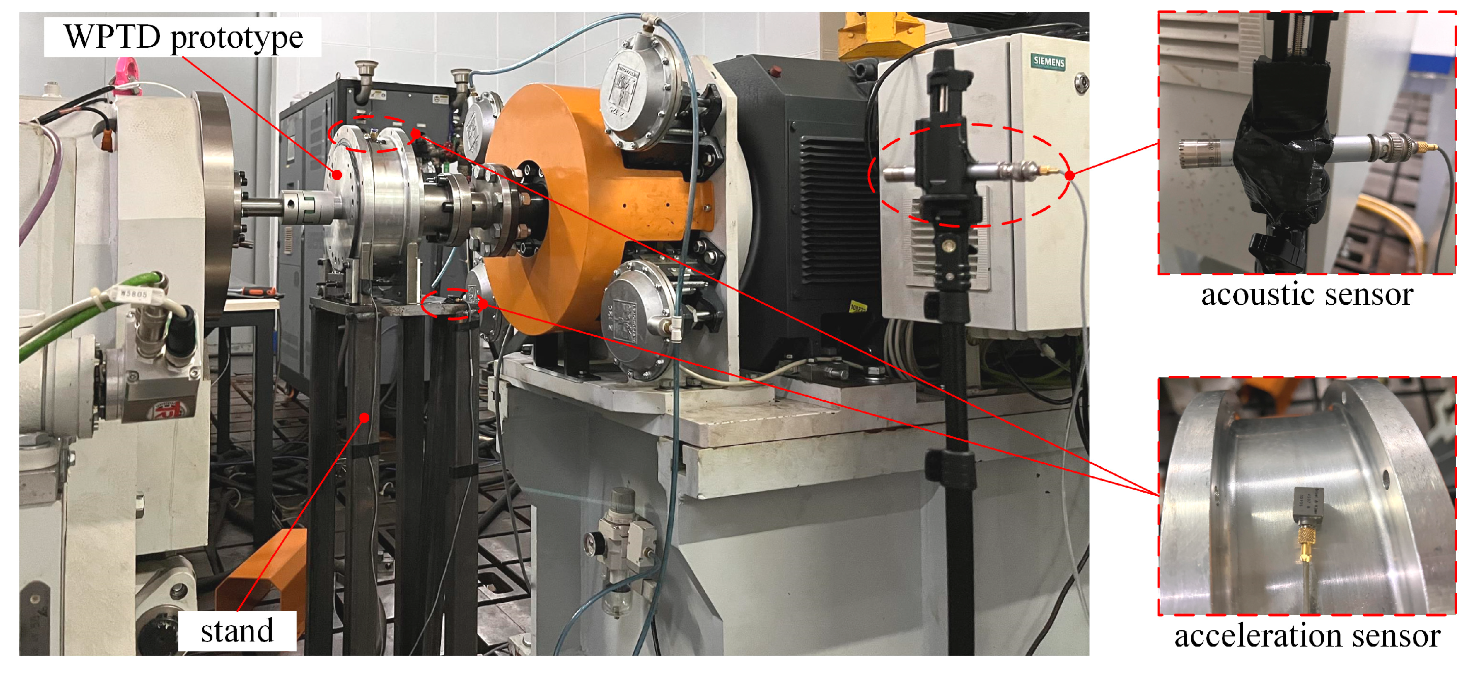
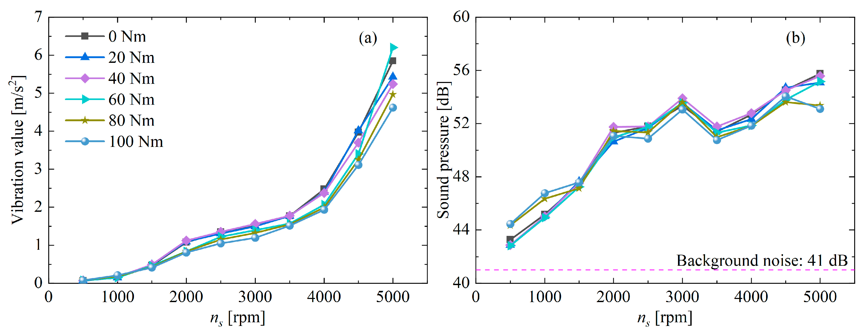
5.3. Vibration and Noise Tests

To measure the vibration and noise levels of the WPTD prototype, acceleration sensors were attached to the housing and the stand, while an acoustic sensor was placed 1 m away, facing the prototype (Figure 16). The vibration and noise were recorded while running the prototype at various input speed ns and output torque Tout combinations.
Figure 17 shows the effect of ns and Tout on the overall vibration and noise levels of the prototype. Due to the introduction of more unstable factors and high-frequency components into the system under high-speed conditions, the vibration and noise levels increased with ns. In addition, the loading mechanism produced a greater loading force at high torque, which increased the contact stiffness and effectively inhibited the vibration. Consequently, the vibration and noise levels generally show a downward trend as Tout increases.
Figure 18 compares the vibration levels of the WPTD prototype and the gear transmission (experimental data were provided by the NSK company), both transmitting a 100 Nm torque. The vibration level of the gear transmission far exceeds that of the WPTD prototype. For example, when n s = 5000   rpm , the approximate vibration level of the gear transmission was 8.0 m/s2, while that of the WPTD prototype was 4.8 m/s2. The WPTD prototype exhibited substantially lower vibration levels, possibly due to the absence of vibration noise associated with gear meshing in traction drives. In addition, the tangential compliance of the EHD fluid film between contacting rollers, together with the elastic compliance of the rollers themselves, provided an effective damping action to further reduce vibrational disturbances. Therefore, WPTD has a significantly lower vibration signature with its vibration levels reduced by more than 40% compared to gear transmission.
The proposed WPTD was subjected to a series of performance tests, including efficiency tests and vibration and noise tests. Along with the prototype performance test, the temperature stability test was conducted using thermocouples attached to the outer surface of the housing. The results show that the maximum temperatures stabilize at about 40 °C (room temperature 22 °C), indicating WPTD’s satisfactory temperature performance. In addition, no obvious change was observed in the surface roughness at each contact pair after performance tests, confirming the good operating conditions of the prototype in the test. The stable temperature and good operation further ensure the reliability of the test data. The test results confirmed that WPTD exhibited an overall efficiency of up to 96% and showed smooth power-transfer characteristics in terms of vibration and noise. Therefore, WPTD is expected to be a cheaper, quieter, and more efficient alternative to high-speed gear drives.

6. Conclusions

This study proposed a new WPTD that could achieve zero spins, a large speed ratio, and self-adaptive loading. A refined theoretical analysis model was established for traction drive performance evaluation and design optimization, which could adapt to a wide range of operating conditions for almost any line-contact traction drive configuration. On this basis, the loading performance, transmission characteristics, and the influence of different parameters on the transmission characteristics of WPTD were analyzed. In addition, prototype performance tests were conducted to verify the theoretical results. The conclusions are drawn as follows:
  • According to the general traction drive operating conditions, the mixed thermal EHL model was adopted for the first time to analyze traction performance, and regression analyses were performed based on the results of extensive simulations. Then, the fitting formulas were derived to predict the film thickness, asperity load ratio, and traction coefficient with provision for both hydrodynamic and surface asperity effects. The results demonstrate the high prediction accuracy of the fitting formulas;
  • A theoretical analysis model considering the combined effects of elastic deformation, loading state, and mixed thermal EHL was established, based on the structural characteristics of WPTD and the new loading principle, and an efficient and accurate performance-prediction method was proposed for traction drives. The theoretical analysis model can simulate the traction capacity and transmission efficiency through numerical calculation;
  • The loading effect was investigated in terms of the traction coefficient, creep coefficient, and efficiency. The results showed that the proposed loading mechanism could achieve self-adaptive loading while maintaining a stable traction coefficient and avoiding slippage, reflecting its good loading effect and improved torque capacity and efficiency;
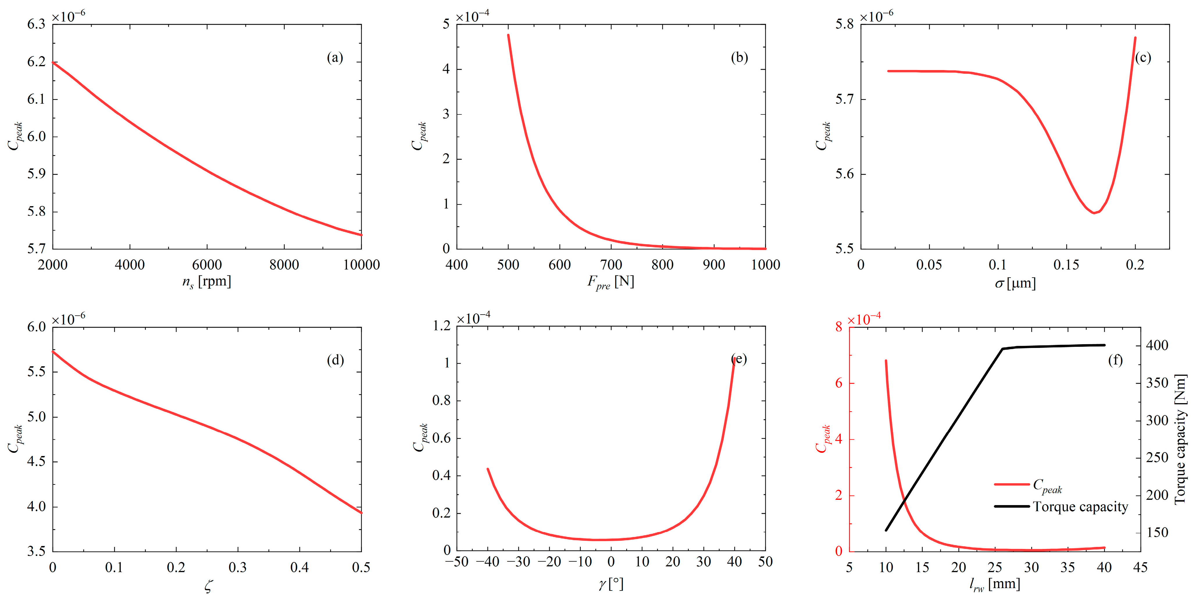
  • The reasonable parameter design can improve the performance of WPTD and reduce sliding. It was confirmed that the preload force Fpre, characteristic angle γ, and contact length lrw exhibit the most significant effects on the global sliding coefficient. Therefore, these parameters deserve special attention during design to avoid transmission failure due to excessive slippage. Meanwhile, the creep coefficient variation is closely related to the loading state. These findings provide new ideas for the future design and optimization of traction drives;
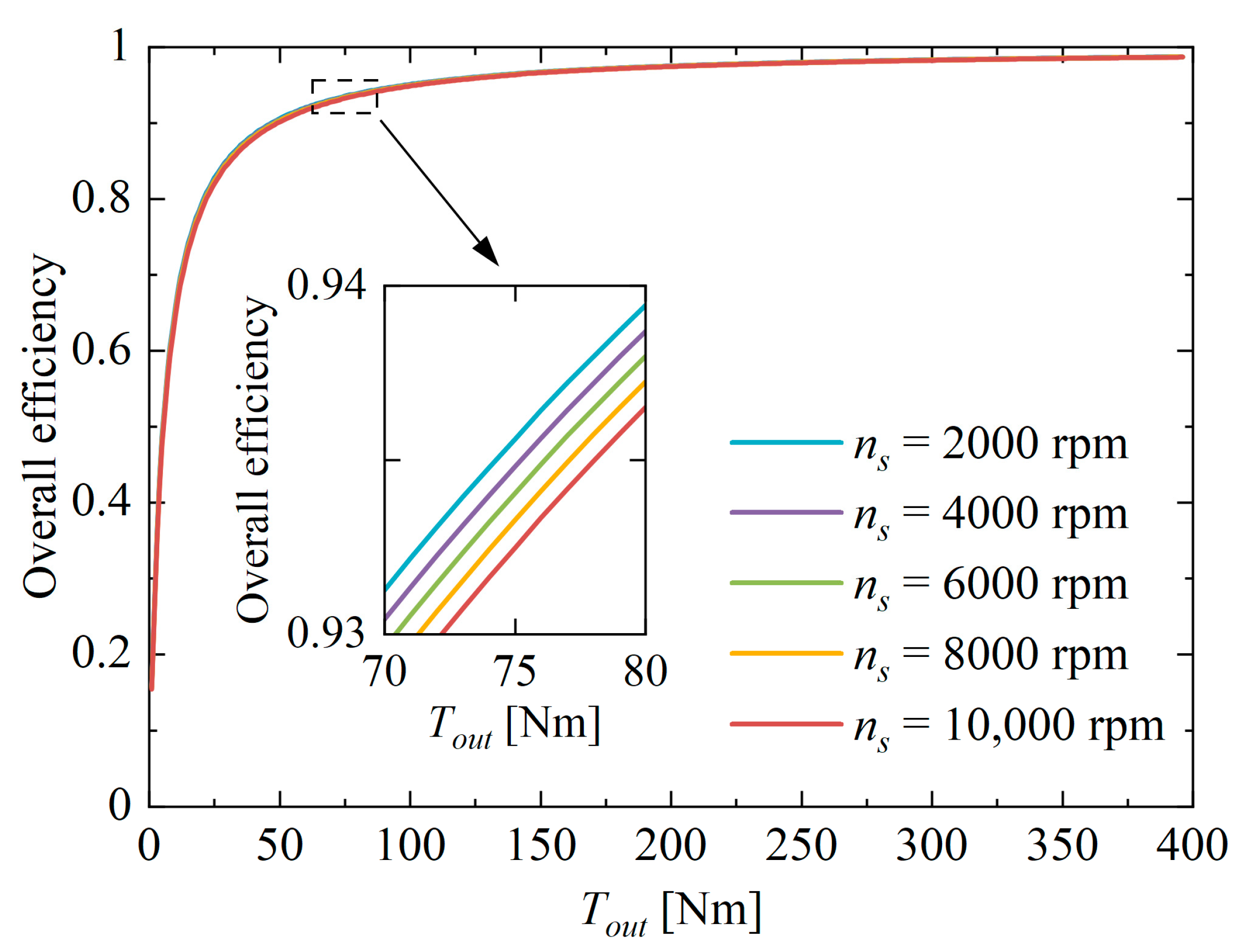
  • Through performance tests on the WPTD prototype, the simulation results are in reasonably good agreement with the experimental data, with the maximum efficiency error less than 9%, validating the theoretical model. The speed is found to have little effect on efficiency, while its increments can significantly increase the power density of WPTD. In addition, the test results confirm the smooth power-transfer characteristics of WPTD, with its vibration levels reduced by more than 40% compared to gear transmission. Benefiting from the zero-spin design and good loading effect, WPTD achieves a peak efficiency of 96%, and delivers superior performance in terms of high-speed potential, transmission efficiency, and vibration noise.
This study analyzed the WPTD at a steady state and validated the theoretical model through prototype tests to enrich the theoretical design system of traction drives and to provide a basis for the design and research of subsequent T-FRTs. WPTD is worth further research and development in high-speed, high-efficiency, and low-vibration transmission. In addition, a traction-contact model considering material evolution and wear mechanism, the dynamic analysis of the transmission and loading mechanisms, and design solutions for different application fields will be key topics for subsequent research. It should be noted that this study is not an attempt to prove WPTD is the best form of T-FRTs. Its purpose is to demonstrate that traction drives should be viewed as a possible solution for developing competitive high-speed transmission systems so that the potential benefits of increased motor speed can be utilized in more applications (e.g., electric vehicles and aerospace).

Author Contributions

Conceptualization, Y.J. and G.W.; methodology, Y.J.; validation, Y.J. and G.W.; investigation, Y.J.; resources, G.W.; writing—original draft preparation, Y.J.; writing—review and editing, G.W.; supervision, G.W.; project administration, G.W. All authors have read and agreed to the published version of the manuscript.

Funding

This research was funded by National Natural Science Foundation of China (grant no. 92048201).

Data Availability Statement

The datasets supporting the conclusions of this article are included within the article.

Conflicts of Interest

The authors declare no conflicts of interest.

Nomenclature

SymbolDefinitionUnit
c p Specific heat capacity of lubricantJ/(kg·K)
C Global sliding coefficient-
C p e a k The peak of the global sliding coefficient-
C j k Creep coefficient in the contact area between part j and part k-
D Density–temperature coefficientK−1
E Effective elasticity modulusPa
f c Asperity friction coefficient-
F c Contact force on planet carrier groove surfaceN
F p r e Initial preload forceN
F j k , F t j k Normal force and traction force between part j and part kN
F t a , F t h Asperity friction force and hydrodynamic traction forceN
h Film thicknessm
h c , h min Central film thickness and minimum film thicknessm
h d Vickers hardnessPa
h T Average gap between two surfacesm
k Thermal conductivity of lubricantW/(m·K)
l j k Contact length between part j and part km
L a Asperity load ratio-
m Limiting shear stress coefficient-
M j Mass of the part jkg
n s Input speed of sun rollerr/min
N Number of planet rollers-
p , p a , p h Total pressure, asperity pressure and hydrodynamic pressure in the contact areaPa
P i n , P o u t Input power and output powerW
P l Overall power lossW
q Mass flow ratekg/s
r j Radius of part jm
R Equivalence contact radiusm
S Slide-to-roll ratio-
S c I D , S c Ideal speed ratio and actual speed ratio when the planet carrier outputs the power-
T , T 0 Film temperature and ambient temperatureK
T B Bearing frictional momentN·m
T o u t Output torqueN·m
u , u z Flow velocity along x and z axesm/s
w Loading force per contact lengthN/m
x i , x e Inlet and outlet position of the lubricantm
z Viscosity–pressure index-
α 0 Viscosity–pressure coefficient-
α , β , γ , φ The defined characteristic angles (Figure 2)°
ω j Angular velocity of part jrad/s
σ Standard deviation of the surface heightsm
δ j k Elastic deformation between part j and part km
ϕ x Pressure flow factor in x direction-
τ 0 Limiting shear stress at atmospheric pressurePa
ζ Starvation degree-
μ Traction coefficient-
ρ Lubricant densitykg/m3
η Lubricant viscositypa·s
η o v e r a l l Overall efficiency-

Appendix A

Table A1. A part of results from simulations (Sim) and fitting formulas (Fit) as well as their corresponding errors (Er).
Input H min H c L a μ
W U σ ¯ K S ζ Sim   ( Fit ) × 10 5 Er (%) Sim   ( Fit ) × 10 5 Er (%)Sim (Fit) %Er (%)Sim (Fit)Er
3.2 × 10 5 3.2 × 10 11 6.2 × 10 5 1.9 × 10 9 1 × 10 8 06.1935 (6.4123)3.536.8173 (6.6825)1.9854.93 (54.11)0.820.0666 (0.0649)0.0017
1 × 10 5 06.1941 (6.3398)2.356.8182 (6.7356)1.2154.92 (54.11)0.810.0665 (0.0649)0.0016
1 × 10 2 06.1833 (6.0969)1.406.8090 (6.8458)0.5455.04 (54.11)0.930.0672 (0.0659)0.0013
2 × 10 4 3.2 × 10 11 6.2 × 10 5 1.9 × 10 9 1 × 10 8 05.1340 (5.1870)1.035.2761 (5.2458)0.5726.39 (26.40)0.010.0319 (0.0326)0.0007
1 × 10 5 05.1346 (5.1251)0.195.2765 (5.2912)0.2826.39 (26.40)0.010.0701 (0.0668)0.0033
1 × 10 2 04.9468 (4.9179)0.585.4409 (5.3855)1.0226.01 (26.40)0.390.1016 (0.0994)0.0022
5 × 10 4 7.5 × 10 11 6.2 × 10 5 1.9 × 10 9 1 × 10 8 07.1738 (7.2189)0.637.4272 (7.4154)0.169.30 (8.80)0.500.0843 (0.0892)0.0049
1 × 10 5 07.1062 (7.1195)0.197.5906 (7.4880)1.359.10 (8.80)0.300.0963 (0.0947)0.0016
1 × 10 2 06.6007 (6.7864)2.817.8411 (7.6388)2.588.28 (8.80)0.520.0991 (0.0949)0.0042
2.6 × 10 4 1 × 10 11 2.4 × 10 5 2.4 × 10 9 1 × 10 8 02.2140 (2.2431)1.312.2771 (2.3117)1.5218.86 (17.85)1.010.0262 (0.0341)0.0079
1 × 10 5 02.2138 (2.2147)0.042.2777 (2.3327)2.4118.86 (17.85)1.010.0856 (0.0937)0.0081
1 × 10 2 02.0087 (2.1197)5.532.3666 (2.3763)0.4118.46 (17.85)0.610.1001 (0.0973)0.0028
2.6 × 10 4 7.5 × 10 11 5.3 × 10 5 2.4 × 10 9 1 × 10 8 07.2679 (7.4256)2.177.6284 (7.7036)0.998.49 (7.66)0.830.0375 (0.0402)0.0027
1 × 10 5 07.2648 (7.3203)0.767.6493 (7.7803)1.718.47 (7.66)0.810.0880 (0.0921)0.0041
1 × 10 2 06.8085 (6.9678)2.348.0417 (7.9397)1.277.89 (7.67)0.220.0983 (0.0945)0.0038
3.44 × 10 4 4.6 × 10 11 5 × 10 6 3.3 × 10 9 1 × 10 8 04.4051 (4.3360)1.574.9242 (4.8938)0.620.00 (0.00)0.000.0733 (0.0803)0.0070
1 × 10 5 04.3664 (4.2613)2.414.9848 (4.9486)0.730.00 (0.00)0.000.0927 (0.0921)0.0006
1 × 10 2 03.8718 (4.0109)3.595.2739 (5.0622)4.010.00 (0.07)0.070.0974 (0.0925)0.0049
3.44 × 10 4 4.6 × 10 11 4 × 10 5 3.3 × 10 9 1 × 10 8 05.1583 (5.1962)0.735.3989 (5.3943)0.098.51 (8.06)0.450.0689 (0.0771)0.0082
1 × 10 5 05.1445 (5.1215)0.455.4526 (5.4490)0.078.43 (8.06)0.370.0925 (0.0943)0.0018
1 × 10 2 04.7407 (4.8711)2.755.7895 (5.5627)3.927.68 (8.06)0.380.0990 (0.0947)0.0043
3.2 × 10 4 1.5 × 10 11 1.6 × 10 5 1.6 × 10 9 1 × 10 8 0.192.1171 (2.2200)4.862.1725 (2.2505)3.598.48 (6.62)1.860.0644 (0.0532)0.0112
1 × 10 5 0.192.1016 (2.1906)4.232.2017 (2.2747)3.328.52 (6.60)1.920.0916 (0.0922)0.0006
1 × 10 2 0.191.9856 (2.0828)4.902.2879 (2.3153)1.207.97 (6.68)1.290.0989 (0.0943)0.0046
1.5 × 10 4 2.3 × 10 11 1 × 10 5 2.2 × 10 9 1 × 10 8 0.392.1598 (2.2796)5.552.2099 (2.2051)0.221.91 (0.97)0.940.0033 (0.0038)0.0005
1 × 10 5 0.392.1598 (2.2441)3.902.2100 (2.2282)0.821.91 (1.04)0.870.0733 (0.0618)0.0115
1 × 10 2 0.402.0290 (2.1171)4.342.2674 (2.2646)0.121.80 (3.32)1.520.0974 (0.0921)0.0053

References

  1. Tenconi, A.; Vaschetto, S.; Vigliani, A. Electrical Machines for High-Speed Applications: Design Considerations and Tradeoffs. IEEE Trans. Ind. Electron. 2014, 61, 3022–3029. [Google Scholar] [CrossRef]
  2. Shen, J.; Qin, X.; Wang, Y. High-Speed Permanent Magnet Electrical Machines—Applications, Key Issues and Challenges. CES Trans. Electr. Mach. Syst. 2018, 2, 11. [Google Scholar] [CrossRef]
  3. Lopez, I.; Ibarra, E.; Matallana, A.; Andreu, J.; Kortabarria, I. Next generation electric drives for HEV/EV propulsion systems: Technology, trends and challenges. Renew. Sustain. Energ. Rev. 2019, 114, 109336. [Google Scholar] [CrossRef]
  4. Fodorean, D.; Idoumghar, L.; Brevilliers, M.; Minciunescu, P.; Irimia, C. Hybrid Differential Evolution Algorithm Employed for the Optimum Design of a High-Speed PMSM Used for EV Propulsion. IEEE Trans. Ind. Electron. 2017, 64, 9824–9833. [Google Scholar] [CrossRef]
  5. Wu, Z.; Li, W.; Tang, H.; Luo, S.; Zhang, L. Research on the Calculation of Rotor’s Convective Heat Transfer Coefficient of High-Speed Drive Motor for EVs Based on Multiple Scenarios. J. Electr. Eng. Technol. 2023, 18, 4245–4256. [Google Scholar] [CrossRef]
  6. Ouyang, T.; Huang, H.; Zhang, N.; Mo, C.; Chen, N. A model to predict tribo-dynamic performance of a spur gear pair. Tribol. Int. 2017, 116, 449–459. [Google Scholar] [CrossRef]
  7. Lei, Y.; Hou, L.; Fu, Y.; Hu, J.; Chen, W. Research on vibration and noise reduction of electric bus gearbox based on multi-objective optimization. Appl. Acoust. 2020, 158, 107037. [Google Scholar] [CrossRef]
  8. Sun, M.; Lu, C.; Liu, Z.; Sun, Y.; Chen, H.; Shen, C. Classifying, Predicting, and Reducing Strategies of the Mesh Excitations of Gear Whine Noise: A Survey. Shock. Vib. 2020, 2020, 1–20. [Google Scholar] [CrossRef]
  9. Kim, B.; Oh, S.; Park, S. Manufacture of elastic composite ring for planetary traction drive with silicon rubber and carbon fiber. Compos. Struct. 2004, 66, 543–546. [Google Scholar] [CrossRef]
  10. Itagaki, H.; Ohama, K.; Raja Rajan, A.N. Method for estimating traction curves under practical operating conditions. Tribol. Int. 2020, 149, 105639. [Google Scholar] [CrossRef]
  11. Ai, X. Development of zero-spin planetary traction drive transmission: Part 1—Design and principles of performance calculation. J. Tribol. 2002, 124, 386–391. [Google Scholar] [CrossRef]
  12. Ai, X. Development of zero-spin planetary traction drive transmission: Part 2—Performance testing and evaluation. J. Tribol. 2002, 124, 392–397. [Google Scholar] [CrossRef]
  13. Ai, X.; Wilmer, M.; Lawrentz, D. Development of Friction Drive Transmission. J. Tribol. 2005, 127, 857–864. [Google Scholar] [CrossRef]
  14. Yamanaka, M.; Sugimoto, K.; Hashimoto, R.; Inoue, K. Intelligent speed-increasing spindle using traction drive. Precis. Eng.-J. Int. Soc. Precis. Eng. Nanotechnol. 2011, 35, 191–196. [Google Scholar] [CrossRef]
  15. Flugrad, D.R.; Qamhiyah, A.Z. A self-actuating traction-drive speed reducer. J. Mech. Des. 2005, 127, 631–636. [Google Scholar] [CrossRef]
  16. Wang, W.; Durack, J.M.; Durack, M.J.; Zhang, J.; Zhao, P. Automotive Traction Drive Speed Reducer Efficiency Testing. Automot. Innov. 2021, 4, 81–92. [Google Scholar] [CrossRef]
  17. Jiang, Y.; Wang, G.; Luo, Q.; Zou, S. Asymmetric loading multi-roller planetary traction drive: Modeling and performance analysis. Mech. Mach. Theory 2022, 170, 104697. [Google Scholar] [CrossRef]
  18. Li, C.; Wang, G.; Jiang, Y.; Song, H. A novel traction reducer: Analysis and verification. J. Adv. Mech. Des. Syst. 2024, 18, JAMDSM0017. [Google Scholar] [CrossRef]
  19. Nikas, G.K. Miscalculation of film thickness, friction and contact efficiency by ignoring tangential tractions in elastohydrodynamic contacts. Tribol. Int. 2017, 110, 252–263. [Google Scholar] [CrossRef]
  20. De Novellis, L.; Carbone, G.; Mangialardi, L. Traction and efficiency performance of the double roller full-toroidal variator: A comparison with half- and full-toroidal drives. J. Mech. Des. 2012, 134, 071005. [Google Scholar] [CrossRef]
  21. Carbone, G.; Mangialardi, L.; Mantriota, G. A comparison of the performances of full and half toroidal traction drives. Mech. Mach. Theory 2004, 39, 921–942. [Google Scholar] [CrossRef]
  22. Johnson, K.L.; Greenwood, J.A.; Poon, S.Y. Simple Theory of Asperity Contact in Elastohydrodynamic Lubrication. Wear 1972, 19, 91–108. [Google Scholar] [CrossRef]
  23. Patir, N.; Cheng, H.S. An Average Flow Model for Determining Effects of Three-Dimensional Roughness on Partial Hydrodynamic Lubrication. J. Lubr. Technol. 1978, 100, 12–17. [Google Scholar] [CrossRef]
  24. Masjedi, M.; Khonsari, M.M. Film thickness and asperity load formulas for line-contact elastohydrodynamic lubrication with provision for surface roughness. J. Tribol. 2012, 134, 011503. [Google Scholar] [CrossRef]
  25. Damiens, B.; Venner, C.H.; Cann, P.M.E.; Lubrecht, A.A. Starved lubrication of elliptical EHD contacts. J. Tribol. Trans. ASME 2004, 126, 105–111. [Google Scholar] [CrossRef]
  26. Masjedi, M.; Khonsari, M.M. A study on the effect of starvation in mixed elastohydrodynamic lubrication. Tribol. Int. 2015, 85, 26–36. [Google Scholar] [CrossRef]
  27. Kumar, P.; Khonsari, M. Effect of Starvation on Traction and Film Thickness in Thermo-EHL Line Contacts with Shear-Thinning Lubricants. Tribol. Lett. 2008, 32, 171–177. [Google Scholar] [CrossRef]
  28. Ali, F.; Krupka, I.; Hartl, M. An Approximate Approach to Predict the Degree of Starvation in Ball-Disk Machine Based on the Relative Friction. Tribol. Trans. 2013, 56, 681–686. [Google Scholar] [CrossRef]
  29. Ali, F.; Krupka, I.; Hartl, M. Analytical and experimental investigation on friction of non-conformal point contacts under starved lubrication. Meccanica 2013, 48, 545–553. [Google Scholar] [CrossRef]
  30. Ebner, M.; Yilmaz, M.; Lohner, T.; Michaelis, K.; Höhn, B.R.; Stahl, K. On the effect of starved lubrication on elastohydrodynamic (EHL) line contacts. Tribol. Int. 2018, 118, 515–523. [Google Scholar] [CrossRef]
  31. Beheshti, A.; Aghdam, A.B.; Khonsari, M.M. Deterministic surface tractions in rough contact under stick-slip condition: Application to fretting fatigue crack initiation. Int. J. Fatigue 2013, 56, 75–85. [Google Scholar] [CrossRef]
  32. Pei, J.; Han, X.; Tao, Y.; Feng, S. Mixed elastohydrodynamic lubrication analysis of line contact with Non-Gaussian surface roughness. Tribol. Int. 2020, 151, 13. [Google Scholar] [CrossRef]
  33. Greenwood, J.A.; Williamson, J.B. Contact of Nominally Flat Surfaces. Proc. R. Soc. Lond. A Math. Phys. Sci. 1966, 295, 300–319. [Google Scholar] [CrossRef]
  34. Chang, W.R.; Etsion, I.; Bogy, D.B. An elastic-plastic model for the contact of rough surfaces. J. Tribol. Trans. ASME 1987, 109, 257–263. [Google Scholar] [CrossRef]
  35. Zhao, Y.; Maietta, D.M.; Chang, L. An asperity microcontact model incorporating the transition from elastic deformation to fully plastic flow. J. Tribol. Trans. ASME 2000, 122, 86–93. [Google Scholar] [CrossRef]
  36. Beheshti, A.; Khonsari, M.M. Asperity micro-contact models as applied to the deformation of rough line contact. Tribol. Int. 2012, 52, 61–74. [Google Scholar] [CrossRef]
  37. McCool, J.I. Relating Profile Instrument Measurements to the Functional Performance of Rough Surfaces. J. Tribol. Trans. ASME 1987, 109, 264–270. [Google Scholar] [CrossRef]
  38. Masjedi, M.; Khonsari, M.M. Theoretical and experimental investigation of traction coefficient in line-contact EHL of rough surfaces. Tribol. Int. 2014, 70, 179–189. [Google Scholar] [CrossRef]
  39. Kumar, P.; Khonsari, M.M. Combined effects of shear thinning and viscous heating on EHL characteristics of rolling/sliding line contacts. J. Tribol. Trans. ASME 2008, 130, 13. [Google Scholar] [CrossRef]
  40. Bair, S.; Winer, W.O. Rheological model for elastohydrodynamic contacts based on primary laboratory data. J. Lubr. Technol. Trans. ASME 1979, 101, 258–265. [Google Scholar] [CrossRef]
  41. Andersson, S.; Soderberg, A.; Bjorklund, S. Friction models for sliding dry, boundary and mixed lubricated contacts. Tribol. Int. 2007, 40, 580–587. [Google Scholar] [CrossRef]
  42. Popova, E.; Popov, V.L. The research works of Coulomb and Amontons and generalized laws of friction. Friction 2015, 3, 183–190. [Google Scholar] [CrossRef]
  43. Verbelen, F.; Druant, J.; Derammelaere, S.; Vansompel, H.; De Belie, F.; Stockman, K.; Sergeant, P. Benchmarking the permanent magnet electrical variable transmission against the half toroidal continuously variable transmission. Mech. Mach. Theory 2017, 113, 141–157. [Google Scholar] [CrossRef]
  44. Akehurst, S.; Parker, D.A.; Schaaf, S. CVT rolling traction drives—A review of research into their design, functionality, and modeling. J. Mech. Des. 2006, 128, 1165–1176. [Google Scholar] [CrossRef]
  45. Dormois, H.; Fillot, N.; Habchi, W.; Dalmaz, G.; Vergne, P.; Morales-Espejel, G.E.; Ioannides, E. A Numerical Study of Friction in Isothermal EHD Rolling-Sliding Sphere-Plane Contacts With Spinning. J. Tribol. 2010, 132, 021501. [Google Scholar] [CrossRef]
  46. Matsuda, K.; Goi, T.; Tanaka, K.; Imai, H.; Tanaka, H.; Sato, Y. Study on high-speed traction drive CVT for aircraft power generation—Gyroscopic effect of the thrust ball bearing on the CVT. J. Adv. Mech. Des. Syst. 2017, 11, JAMDSM0087. [Google Scholar] [CrossRef]
Figure 1. The structure of WPTD and related geometrical quantities: (a) schematic diagram; (b) kinematic diagram.
Machines 12 00567 g001
Figure 2. (a) Continuous deformation model of the WPTD; (b) the center position of rollers under load.
Machines 12 00567 g002
Figure 3. The loading state analysis of the loading mechanism. The clockwise rotation of the sun roller is taken as an example for analysis.
Machines 12 00567 g003
Figure 4. The free-body diagram of the transmission parts. The clockwise rotation of the sun roller is taken as an example for analysis.
Machines 12 00567 g004
Figure 5. The lubrication state of contact areas.
Machines 12 00567 g005
Figure 6. The calculation flowchart of the mathematical model of WPTD.
Machines 12 00567 g006
Figure 7. The displacement xw of the circular center of wedge rollers as a function of output torque Tout. Input speed of sun roller ns = 10,000 rpm and initial preload force Fpre = 800 N.
Machines 12 00567 g007
Figure 8. (a) Contact force Fc at the groove surface of the planet carrier, and (b) tangential force Ftrw at the ring as a function of output torque Tout. ns = 10,000 rpm and Fpre = 800 N.
Machines 12 00567 g008
Figure 9. (a) The traction coefficient μ as a function of output torque Tout; (b) the global sliding coefficient and the creep coefficient as functions of output torque Tout. ns = 10,000 rpm and Fpre = 800 N.
Machines 12 00567 g009
Figure 10. The overall efficiency ηoverall of WPTD as a function of output torque Tout at different input speeds ns. The efficiency values are calculated with Equations (25) and (28). Fpre = 800 N.
Machines 12 00567 g010
Figure 11. The variation of Cpeak for different parameters: (a) input speed ns; (b) preload force Fpre; (c) surface roughness σ; (d) starvation degree ζ; (e) characteristic angle γ; (f) contact length lrw.
Machines 12 00567 g011
Figure 12. Physical pictures of the WPTD: (a) main transmission components; (b) the prototype.
Machines 12 00567 g012
Figure 13. The test rig for the WPTD prototype.
Machines 12 00567 g013
Figure 14. Comparison of theoretical and experimental results of the overall efficiency ηoverall of the prototype at different input speeds ns: (a) ns = 2000 rpm; (b) ns = 3000 rpm; (c) ns = 4000 rpm; (d) ns = 5000 rpm; (e) ns = 6000 rpm; (f) the peak efficiency ηpeak vs. ns.
Machines 12 00567 g014
Figure 15. Measured efficiency map of the WPTD prototype.
Machines 12 00567 g015
Figure 16. Vibration and noise tests of the WPTD prototype.
Machines 12 00567 g016
Figure 17. Effect of input speed ns and output torque Tout on the overall vibration (a) and noise (b) levels of the WPTD prototype.
Machines 12 00567 g017
Figure 18. Comparison of vibration levels of the WPTD prototype and gear transmission transmitting a 100 Nm output torque at different input speeds.
Machines 12 00567 g018
Table 2. The range of input parameters.
Parameters W U σ ¯ K S ζ
Min3.2 × 10−53 × 10−125 × 10−61.3 × 10900
Max5 × 10−47.5 × 10−111 × 10−47 × 1090.20.5
Table 3. The characteristic parameters of Santotrac 50.
ParametersValues
Lubricant viscosity at atmospheric pressure η 0 = 0.0127   Pa s
Viscosity–pressure index z = 0.85
Pressure–viscosity coefficient α 0 = 2.3 × 10 8   Pa 1
Limiting shear stress at atmospheric pressure τ 0 = 6.5 × 10 6   Pa
Limiting shear stress coefficient m = 0.095
Table 4. The geometric and material parameters.
ParametersValues
Sun roller radius r s = 6.4   mm
Planet roller radius r p = 36.4   mm
Wedge roller radius r w = 8.7   mm
Ring radius r r = 96   mm
Number of planet rollers N = 3
The defined characteristic angles γ γ l = 5.6 , γ r = 5.6
Elastic modulus E = 207.5   GPa
Poisson ratios ν = 0.3
Ideal speed ratio S c I D = 14 , S r I D = 15
Disclaimer/Publisher’s Note: The statements, opinions and data contained in all publications are solely those of the individual author(s) and contributor(s) and not of MDPI and/or the editor(s). MDPI and/or the editor(s) disclaim responsibility for any injury to people or property resulting from any ideas, methods, instructions or products referred to in the content.

