Abstract
The safety and reliability of high-speed train electric traction systems are crucial. However, the operating environment for China Railway High-speed (CRH) trains is challenging, with severe working conditions. Dataset imbalance further complicates fault diagnosis. Therefore, conducting fault diagnosis for high-speed train electric traction systems under data imbalance is not only theoretically important but also crucial for ensuring vehicle safety. Firstly, when addressing the data imbalance issue, the fault diagnosis mechanism based on support vector machines tends to prioritize the majority class when constructing the classification hyperplane. This frequently leads to a reduction in the recognition rate of minority-class samples. To tackle this problem, a self-tuning support vector machine is proposed in this paper by setting distinct penalty factors for each class based on sample information. This approach aims to ensure equal misclassification costs for both classes and achieve the objective of suppressing the deviation of the classification hyperplane. Finally, simulation experiments are conducted on the Traction Drive Control System-Fault Injection Benchmark (TDCS-FIB) platform using three different imbalance ratios to address the data imbalance issue. The experimental results demonstrate consistent misclassification costs for both the minority- and majority-class samples. Additionally, the proposed self-tuning support vector machine effectively mitigates hyperplane deviation, further confirming the effectiveness of this fault diagnosis mechanism for high-speed train electric traction systems.
1. Introduction
The electric traction system is the core power control system of high-speed trains, mainly consisting of a pantograph, traction transformer, traction inverter, traction motor, and transmission gear. The electric traction system of high-speed trains has the highest failure rate among all vehicle control systems, accounting for more than half of all fault types. This poses a significant risk to the safe operation of high-speed trains. Therefore, conducting real-time state monitoring and fault diagnosis of the electric traction system is of great theoretical significance and engineering value in enhancing the safety and reliability of high-speed trains [1].
In the past twenty years, scholars and engineers in the field of safety, both domestically and internationally, have conducted extensive research on fault diagnosis of high-speed train electric traction systems. The mainstream research methods can be categorized into two main types: methods based on analytical models [2] and data-driven methods [3]. The former approach relies on the design of observers and filters, which necessitate the establishment of accurate models, while the latter does not require precise modeling of the system and can automatically learn and adapt to different fault modes. Therefore, data-driven fault diagnosis methods have broader applications. Common data-driven fault diagnosis methods for high-speed train electric traction systems include signal processing [4], statistical analysis [5], artificial intelligence [6], etc. Quantitative diagnosis based on artificial intelligence can be further subdivided into methods such as support vector machine (SVM), neural network, and fuzzy logic. SVM has powerful classification ability, robustness, and interpretability in machine learning-based fault diagnosis methods, and can identify key fault features with relatively low data volume [7]. In order to compensate for the scarcity of sample fault data when classifying high-voltage circuit breaker features, a multi-class relevant vector machine algorithm was designed based on the “one-to-one” multi-class model [8]. A large number of binary relevant vector machine models were trained based on the extracted data features to realize the multiple fault diagnosis. Ref. [9] analyzed the data based on wavelet packet decomposition and reconstruction to calculate the distribution of wavelet packet energy and extract the energy feature of faults. Combined with Genetic Algorithm-Support Vector Machine (GA-SVM), it not only enhanced the classification speed but also improved the classification accuracy. Ref. [10] decomposed the original bearing vibration signal into multiple intrinsic modal functions using the variational mode decomposition (VMD) method, and reconstructed the bearing vibration signal by introducing a feature energy ratio (FER) criterion. By calculating the multiscale entropy of the reconstructed signal to construct multidimensional feature vectors, the constructed multidimensional feature vectors are input into a particle swarm–support vector machine classification model for the identification of different fault modes in rolling bearings. In summary, the above methods are all targeted towards balanced fault datasets, without consideration of imbalanced data conditions. Additionally, in the actual operation of high-speed trains, the proportion of fault data in the overall data is imbalanced. When using the aforementioned data, the issue of imbalance is difficult to avoid, which objectively increases the difficulty of fault diagnosis in the electric traction system.
Imbalanced datasets typically have two conditions: class imbalance and misclassification cost imbalance [11]. The difficulties of the imbalanced data classification problem mainly manifest in the imbalance of the data itself and the limitations of traditional classification algorithms. For data, the number of samples in two classes is unbalanced, making it difficult for classifiers to learn the features of minority-class samples through training. Meanwhile, majority-class samples can blur the boundaries of minority-class samples, making it difficult to distinguish between minority-class samples and majority-class samples in the class overlapping regions. For a classifier, SVM aims to minimize the structural risk and maximize margins. When a dataset is imbalanced, in order to reduce the loss risk, the classification hyperplane will inevitably shift towards the direction of minority-class samples, leading to misclassification of minority-class samples as multiple-class samples in the overlapping regions. Nowadays, fault diagnosis research on imbalanced data mainly focuses on data, fault features, and classification algorithms [12]. For example, in order to eliminate the impact of data imbalance on fault diagnosis accuracy, under-sampling and over-sampling methods were adopted in ref. [13] to balance the data in terms of quantity. However, the under-sampling method may lead to information loss, resulting in reduced learning ability of classifiers for majority-class samples. Ref. [14] enhanced the diagnostic performance by retaining key features of the imbalanced dataset to improve the discrimination between the majority and minority classes, further mitigating the impact of data imbalance from the classifier perspective. However, the diagnostic performance of the model is overly reliant on the rationality of feature selection. Furthermore, improvements in classification algorithms can retain all sample information when addressing data imbalance issues, and the trained model can adapt to various imbalanced datasets, avoiding complex data preprocessing. Ref. [15] proposed a Biased Support Vector Machine (Biased-SVM) model-based scheme. By assigning different penalty factors to the two classes of samples, increasing the penalty factor for the minority-class samples and reducing the penalty factor for the majority-class samples, the problem of low classification accuracy caused by data imbalance is to some extent resolved. Inspired by the above schemes, this paper proposes a self-adjusting support vector machine (St-SVM)-based approach. The specific design steps, relevant evaluation metrics, and the process of analyzing classification performance are also presented. The simulation experiments for CRH2 high-speed trains are conducted on the Traction Drive Control System-Fault Injection Benchmark (TDCS-FIB) platform using three different imbalance ratios to address the data imbalance issue.
2. The Electric Traction System of CRH2 High-Speed Train
The main circuit topology of the electric traction system in CRH2 high-speed trains is shown in Figure 1, where the sensor distribution locations are highlighted in red and green. The traction inverter utilizes an AC-DC-AC structure, consisting of a pulse rectifier, an intermediate DC circuit, and a three-level inverter. The pulse rectifier (highlighted in the red square) converts AC power to DC power (2600∼3000 V) using IGBT as the switching element. The DC power is transmitted to the inverter through the intermediate DC circuit, where the three-level inverter (highlighted in the blue square) adopts a VVVF control mode, providing adjustable three-phase AC power (0∼2300 V, 0∼220 Hz). This enables the speed and torque control of the four asynchronous motors highlighted in the green square with parallel structure.
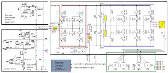
Figure 1.
The electric traction system of a CRH2 high-speed train.
In the electric traction system of high-speed trains, the inverter is a key component that converts DC power to AC power, where the possible causes include: 1. Damage or aging of internal circuit components in the inverter, such as IGBT switching devices and capacitors, which can result in short circuits, open circuits, or voltage abnormalities; 2. Overloading and overheating which can cause the temperature of internal components in the inverter to rise beyond their tolerance limits; 3. Insulation breakdown due to voltage surges or overvoltage. In summary, inverter malfunctions can result in power output fluctuations, leading to unstable train speeds. Additionally, they can trigger faults in other components, such as induction motors, sensors, etc., thereby affecting the normal operation of the entire electric traction system. The sensors in the high-speed train electric traction system may experience sensor drift faults due to environmental factors (especially temperature effects), aging of sensing elements, poor connections, etc., causing the output values to gradually deviate from the actual values. Sensor drift blurs and makes the correlation between faults and sensor output values ambiguous and uncertain, increasing the fault diagnosis complexity. At the same time, the reduced accuracy of sensor data greatly impacts the monitoring of train status.
The high-speed train electric traction system operates under complex and harsh conditions. Conducting physical fault simulation and testing would require a significant amount of time and economic resources, and may lead to equipment damage or even accidents, resulting in unnecessary losses. To address the above-mentioned issues, this study conducts traction system fault simulation and testing based on the TDCS-FIB platform. This simulation platform is constructed based on the physical construction of the CRH2 high-speed train electric traction system. It incorporates functions such as fault injection, control strategy selection, circuit parameter setting, and co-simulation. The platform has garnered recognition and adoption from numerous research teams in the field of fault diagnosis and rail transportation [16]. The simulation platform can simulate various operating conditions, including fault-free scenarios, sensor faults, inverter faults, motor faults, and controller faults. The system dynamics obtained include inverter currents , , , transformer voltages , transformer current , DC-side voltage , train speed , motor speed , and motor electromagnetic torque .
3. Problem Description
For a given dataset , , where represents the i-th sample, the class label of the sample if normal samples, if fault samples. Introducing a kernel function K to handle non-linear problems, a penalty factor C to indicate the degree of penalty, a slack variable to represent the degree of sample misclassification, a parameter w to denote the weight vector of the classification plane, and a parameter b as the bias constant, the general form of SVM can be obtained as
Introducing the Lagrange multiplier method to transform Equation (1) into a dual problem as
and solving for the optimal Lagrange multipliers . According to the KKT conditions, solving for and to derive the decision function as
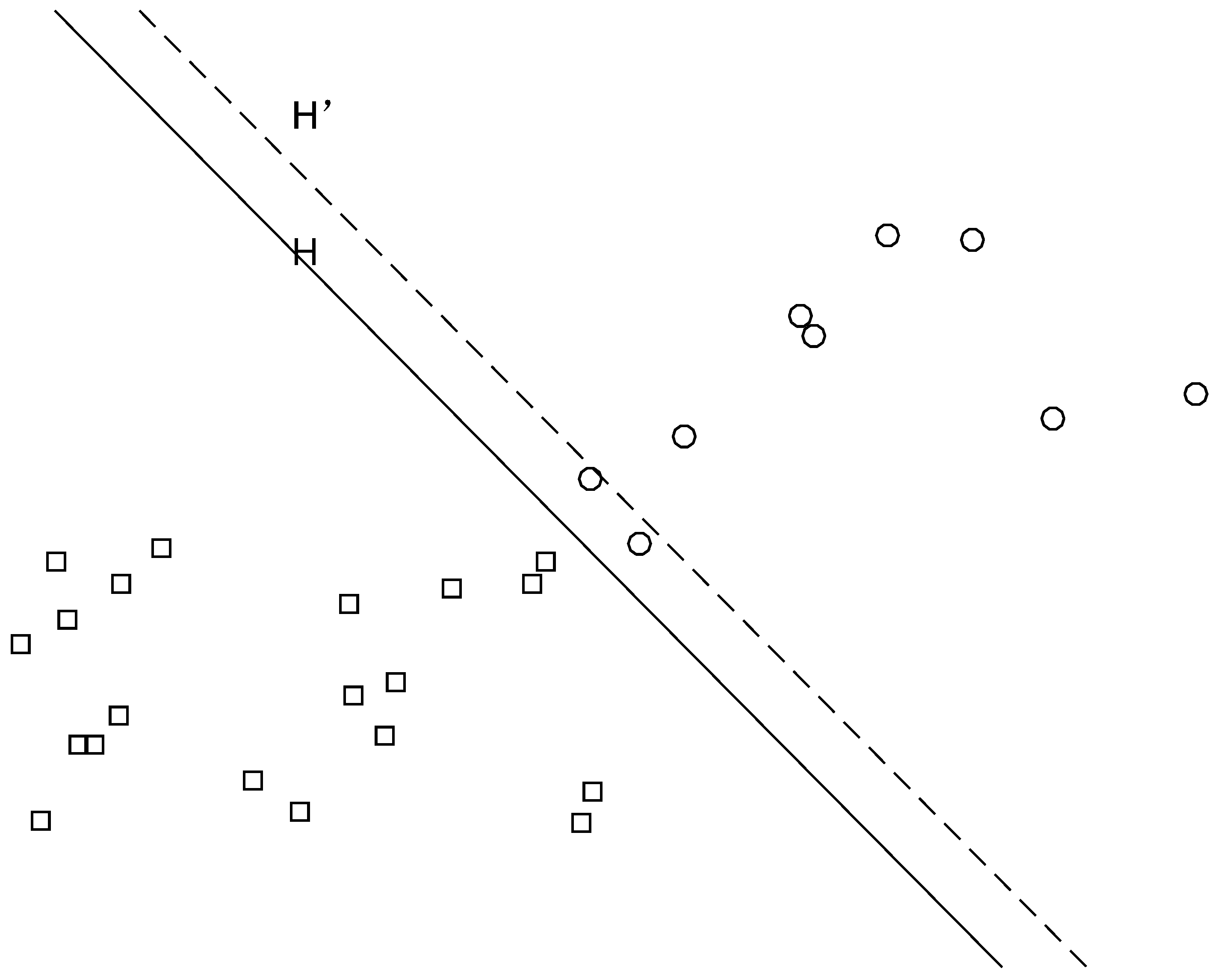
Fault diagnosis based on the SVM algorithm requires that the number of normal samples and fault samples in the dataset be similar. However, in actual operating conditions, the majority of the dataset obtained by sensors on high-speed trains is imbalanced. When dealing with imbalanced data using the SVM algorithm, setting the same penalty factor for all samples may lead to smaller losses for the minority-class samples after training. However, this mechanism of minimizing losses by maximizing the classification margin inevitably causes the classification hyperplane to shift towards the minority-class samples, thus reducing the accuracy of fault diagnosis. As shown in Figure 2, H represents the ideal classification plane. Due to the imbalance of the two classes of samples, the classification hyperplane shifts towards the region of the minority-class samples, where is the shifted hyperplane. It is evident that this classification mechanism reduces the recognition rate of the minority-class samples.
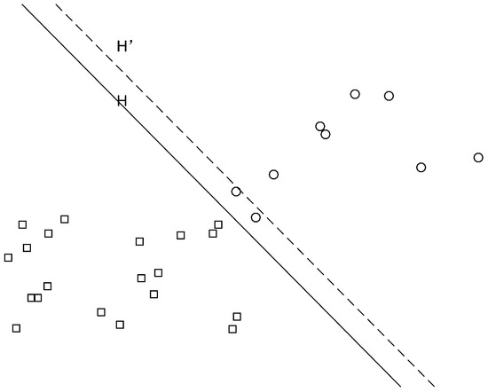
Figure 2.
Sample imbalance leading to hyperplane shift.
To address the classification issue of imbalanced data, the Biasd-SVM method is usually employed by setting different penalty factors for minority- and majority-class samples. By increasing the penalty factor for the minority-class samples, the risk loss of the minority-class samples is elevated, while reducing the penalty factor for the majority-class samples decreases the corresponding risk loss.
For a given dataset, the corresponding minority-class sample set is and the majority-class sample set is , where the total number of samples is l, and the number of minority-class samples is q, , then the Equation (1) can be rewritten as
Similarly, the Equation (4) can be transformed into a dual problem as
where and are penalty factors for the minority and majority-class samples, with .
In Ref. [17], penalty factors for and are determined based on the inverse proportion of the number of majority- and minority-class samples, i.e., . However, the selection of and relies on empirical knowledge, leading to less than ideal results in practical applications. In the Biased-SVM-based scheme, different penalty factors are assigned to different categories of samples, aiming to make the risk loss of both classes as similar as possible, thereby reducing the impact of data imbalance further. Biased-SVM demonstrates improved classification performance compared to traditional SVM when dealing with imbalanced datasets. However, Biasd-SVM only takes into account the differences between different classes, but neglects the variations in information content among samples within the same class. Specifically, the hyperplane of SVM is determined by support vectors, which contain crucial information. Samples that are farther away from the classification hyperplane generally hold less informative content. Assigning the same penalty factor to distinct samples within the same class can lead to inadequate exploitation of the information in the sample space. To address this challenge, the following sections present a Self-tuning Support Vector Machine (St-SVM) strategy. This method autonomously assigns varying penalty factors to individual samples, maximizing the exploitation and utilization of the distributional information in the sample space, consequently suppressing the deviation in the classification hyperplane induced by imbalanced data.
4. Self-Tuning Support Vector Machine
Different samples inherently carry dissimilar amounts of spatial information, necessitating the adaptive adjustment of penalization levels based on their informational content. Distinct penalty factors should be assigned to individual samples to reflect this variation, ensuring a more comprehensive and equitable treatment in the learning process. The St-SVM employs variable penalty factors instead of a constant C. Its general form is depicted as in Equation (6) as
Similarly, Equation (6) can be transformed into a dual problem as
4.1. Self-Tuning Penalty Factor
Step 1: Parameter initialization.
Given l training samples and the number of iterations n, a weight vector is utilized to reflect the information content of each sample, where , . By solving Equation (2), one can obtain the classification hyperplane and the support vectors . Due to the large value of the penalty factor currently, the classification hyperplane can be considered as a hard classification, which has poor generalization ability.
Step 2: Update the information weight vector.
Let the classification error be , where . Update the information weight vector based on Equations (8)–(10) as
It is not difficult to notice that when a sample is classified correctly, its weight is reduced, whereas when a sample is misclassified, its weight will be increased.
Step 3: Generate a new classification hyperplane.
According to Equation (10), a new training set is reconstructed from the training set . Based on Step 1, a new classification hyperplane is obtained.
Step 4: Iterative adjustment.
Steps 2–3 are repeated for n iterations, and the final information weight vector can be obtained. Furthermore, set the penalty factor as
Step 5: Penalty factor normalization.
4.2. Classification Performance
In the case of data imbalance, the suppression of the margin shift in a SVM classifier relies on the ratio of misclassification costs between two classes. The Equation (14) is used to evaluate the suppression ability of a classifier as follows:
where if the value of r is closer to 1, it indicates that the SVM has better capability to resist or correct such shifts. This suggests that the classifier is more effective in maintaining its decision boundary and minimizing misclassification, which is a desired property for a good classification model. The ratio of misclassification loss for minority-class samples to the misclassification loss for majority-class samples in C-SVM for handling imbalanced data classification is shown as follows:
In Biased-SVM, , the ratio of the misclassification loss of minority-class samples to the misclassification loss of majority-class samples can be represented as
where , only when C is a constant. Furthermore, in the St-SVM design,
Substituting Equations (12) and (13) into Equation (14) yields r = 1; the misclassification loss of the two classes of samples remains equal. Comparing St-SVM with C-SVM and Biased-SVM, it is not difficult to find that the St-SVM approach has a better suppression effect on the classification margin shift.
When constructing a classification hyperplane, SVM not only considers the risk loss, but also takes into account the reliability of the resulting classification function.
where is the reliability evaluation function of the classification function, representing the generalization performance of the support vector machine. is directly proportional to . The generalization performance of a classifier can be evaluated as follows:
where represents the risk loss. The larger the value of is, the more the SVM emphasizes generalization ability during training; conversely, the smaller the value of is the more it focuses on learning capability. However, in the St-SVM,
where is inversely proportional to the classification error . Based on the classification results of support vector machines, when the classification accuracy is high, the value of is small, indicating that is large, thus putting more emphasis on generalization performance. Conversely, when the accuracy is lower, it suggests a greater focus on learning capability at the expense of generalization performance.
5. Experiment and Analysis
5.1. Fault Injection in the TDCS-FIB Platform
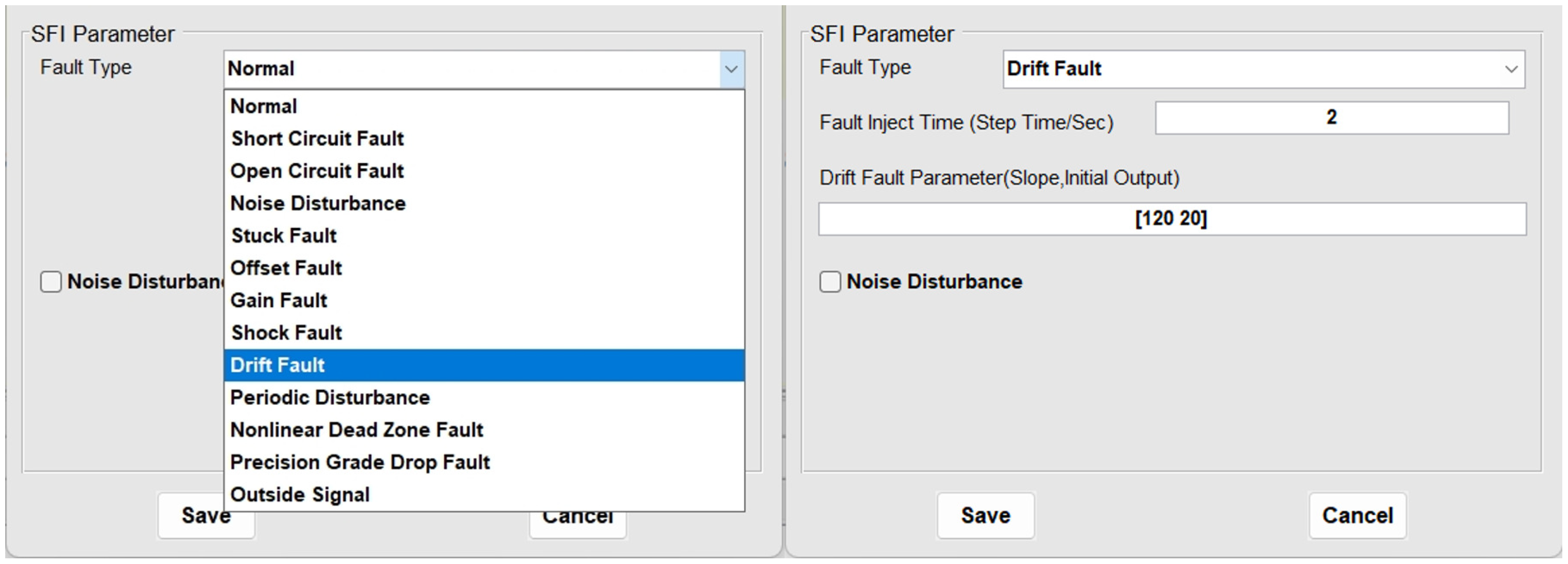
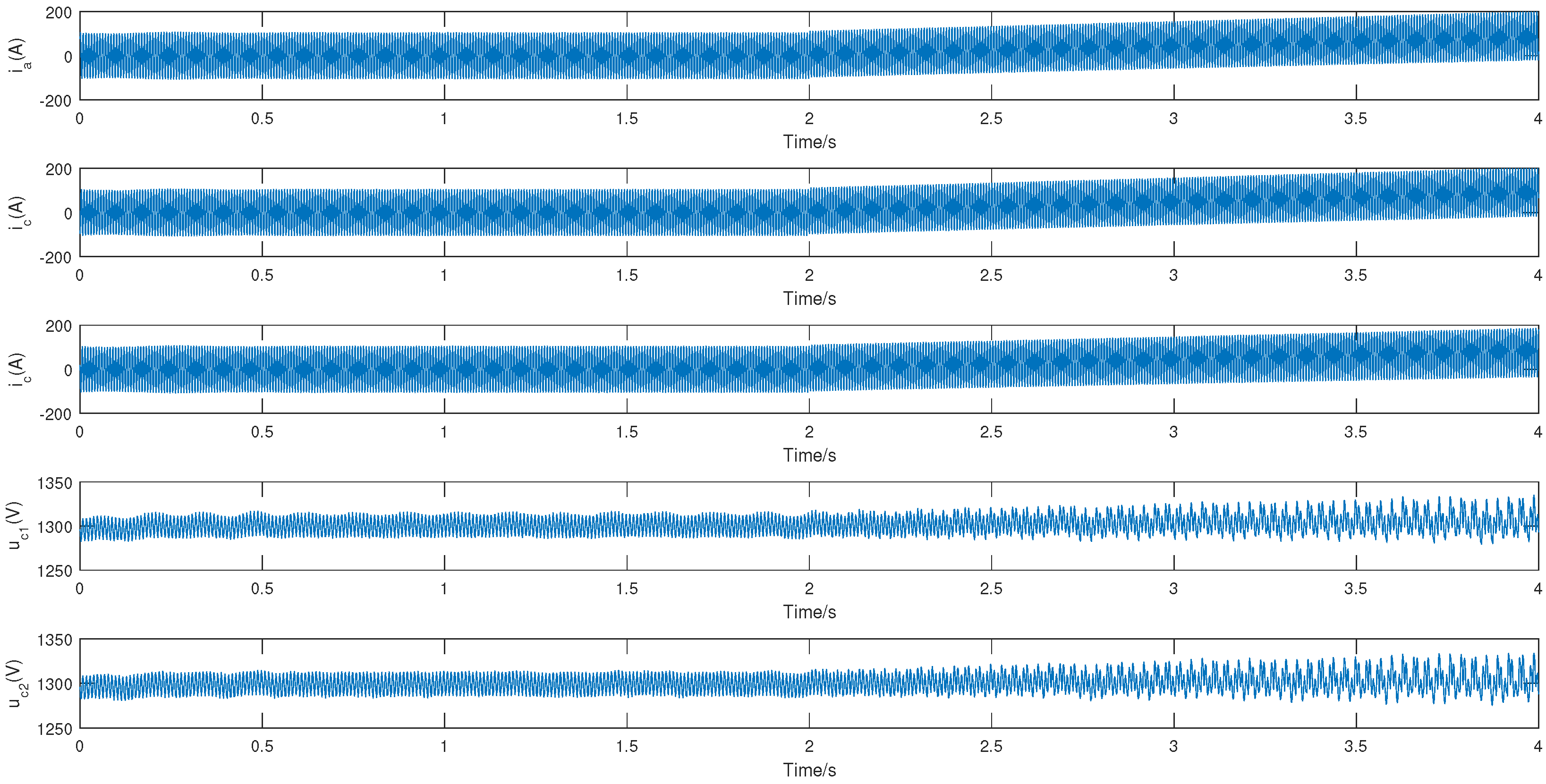
To validate the effectiveness of the proposed algorithm in fault diagnosis of high-speed train traction systems, sensor drift fault injection is used in the TDCS-FIB platform, as shown in Figure 3. The simulation total duration is set to 4 s (1 × samples per second), with the fault injection occurring at the 2nd second. The data selected for the experiment, as shown in Figure 4, includes the inverter currents , , , and DC-side voltages , , both before and after the sensor drift fault. According to the definition of the imbalance ratio (IR), [18], the imbalanced dataset is divided into three categories: a low imbalance dataset (IR: 1.5–3), a medium imbalance dataset (IR: 3–9), and a high imbalance dataset (IR > 9). Based on this criterion, three groups of datasets with different IRs (IR = 2.5, majority class: 100, minority class: 40; IR = 5, majority class: 100, minority class: 20; IR = 10, majority class: 100, minority class: 10) are constructed based on , , and , data in both normal and fault conditions. The signals are divided into window segments consisting of every 2000 sample points. The standard deviation of each signal within these windows is then calculated. This helps in understanding the variability of the signals before and after the sensor drift fault. The standard deviations of the five signals (, , , and ) across each window are arranged into a new dataset. This dataset is then split into a training set and a testing set. The dataset is split into training and testing sets in a ratio of 8:2. Subsequently, normalization is performed on the data to scale the values within the range of 0 and 1, which is a common preprocessing step in many machine learning algorithms to ensure fair comparison and improve model performance.

Figure 3.
Sensor drift fault injection.
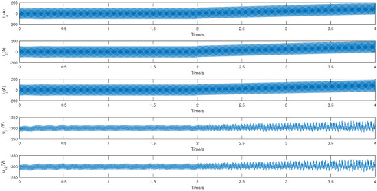
Figure 4.
System dynamics under sensor fault condition.
5.2. Parameter Settings and Evaluation Metrics
The differences among the C-SVM, Biased-SVM and St-SVM described in this paper lie in the selection of the penalty factor C. In order to emphasize the impact of the C adjustment on the classifier performance, all other parameter settings remain identical throughout the experiment, isolating the influence of this particular penalty factor on the classification effectiveness. For the Biased-SVM, the weight is determined on , with class penalty factors , where i represents the sample class label [17]. Meanwhile, for St-SVM, the penalty factor is resolved from Equation (13), where i represents the sample serial number.
For conventional classifiers, accuracy is often selected as the primary metric to evaluate the classification performance. When dealing with imbalanced datasets, the minority-class samples account for a small proportion, thus having less impact on the overall accuracy. Even if all minority-class samples are misclassified into the majority-class, the overall accuracy can still be relatively high. This is why traditional accuracy measures may not adequately reflect the classifier performance, especially in scenarios where correctly identifying minority-classes is crucial. However, when the improved algorithm suppresses the classification margin shift to accurately identify minority-class samples, it might sacrifice more majority-class samples in the process. This could potentially lead to a decrease in the overall accuracy. Therefore, it is a trade-off between the ability to detect minority-class instances and maintaining overall classification performance. In such cases, other evaluation metrics, like recall, the F1-score, or the G-mean, may provide a more comprehensive understanding of the algorithm effectiveness. While paying attention to the recognition rate of minority-class samples, one must also consider the accuracy of majority-class samples. Therefore, in order to provide a more comprehensive assessment of the classifier performance, this paper proposes a composite evaluation metric based on the confusion matrix. In a binary classification problem, where the minority-class of interest is defined as the positive-class and the majority-class as the negative-class, the confusion matrix is as shown in Table 1, where TP represents the prediction result of positive samples as positive, FN represents the prediction result of positive samples as negative, FP represents the prediction result of negative samples as positive, and TN represents the prediction result of negative samples as negative.

Table 1.
Confusion matrix.
Furthermore, the following indicators can be constructed as
where and , respectively, represent the rates of correctly predicted positive and negative class samples. Considering their interdependence, especially when dealing with imbalanced data, it can be challenging to directly evaluate the classification performance using both metrics simultaneously. The evaluation metric takes into account this trade-off between the two aspects. The value decreases when the classifier leans towards one class of samples, making it a more informative measure in such scenarios.
5.3. Diagnostic Performance Analysis
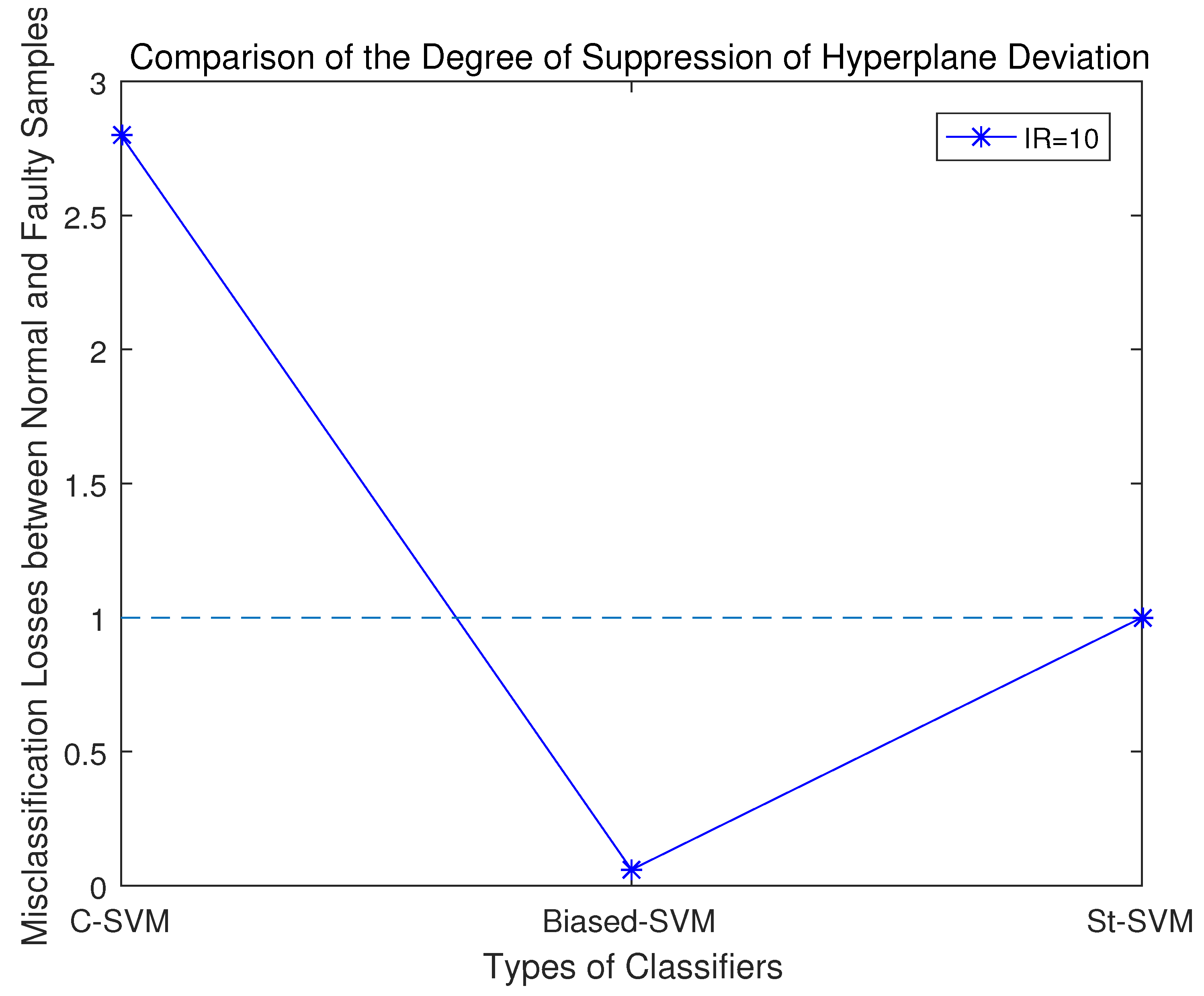
According to the experimental results, the misclassification loss of normal samples and fault samples in these three classifiers was statistically analyzed. Among them, the closer r is to 1, the stronger the classifier’s capability to suppress the classification margin shift.
Comparing the misclassification loss ratios of normal samples and fault samples by the three SVM classifiers, as shown in Figure 5, it becomes clear that: 1. With the traditional SVM, the disparity in the misclassification loss between normal samples and anomalous ones is the most substantial, suggesting that it exhibits the severest classification margin shift towards the minority-class samples; 2. When configuring the Biased-SVM with a penalty factor, the differences in information content among samples are not taken into account. Consequently, in the process of seeking the classification hyperplane, the algorithm overly emphasizes minority-class samples, leading to a classification margin shift towards the majority-class. As a result, while effectively identifying minority-class samples, it misclassifies a significant number of majority-class samples; 3. In the St-SVM, the misclassification loss ratio of normal samples and faulty samples is 1, effectively suppressing the classification margin shift.
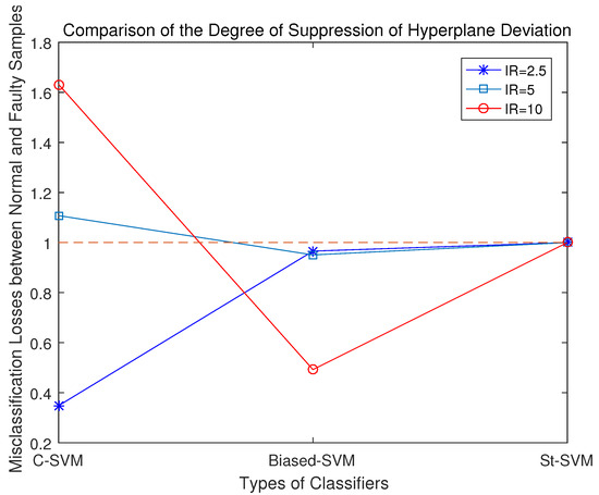
Figure 5.
Comparisons of misclassification losses with different classifiers.
Upon summarizing the results from these three experimental sets, it becomes evident that the degree of classification margin shift of the conventional SVM increases as the data imbalance ratio grows. The Biased-SVM often suppresses the classification margin shift excessively. On the other hand, the St-SVM consistently maintains an equal misclassification loss for both normal and fault samples, resulting in a ratio of 1.
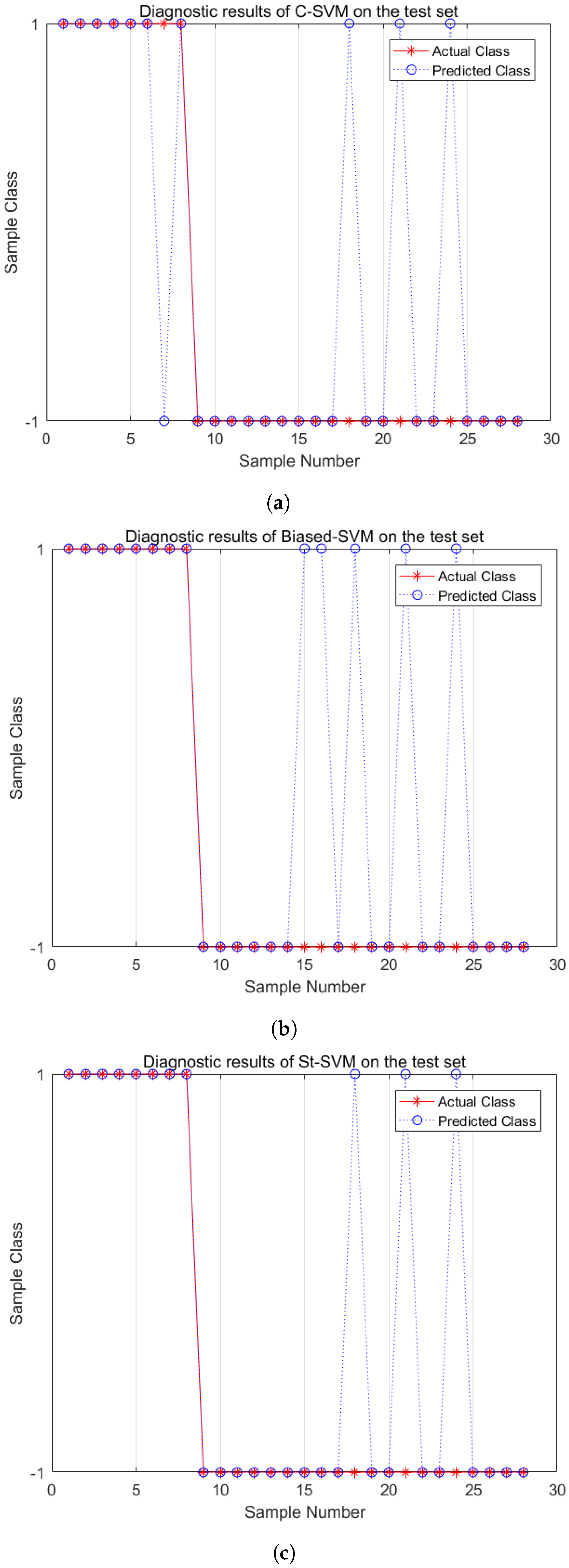
Figure 6 shows the fault diagnosis results of the test dataset based on C-SVM, Biased-SVM, and St-SVM with low imbalance data (IR = 2.5). From the experimental results, the C-SVM misclassifies one minority-class sample and three majority-class samples. The Biased-SVM identifies all minority-class samples but misclassifies five majority-class samples. The St-SVM not only identifies all minority-class samples but also misclassifies only three majority-class samples. Therefore, the St-SVM performs the best in fault diagnosis under the condition of handling low imbalance data.
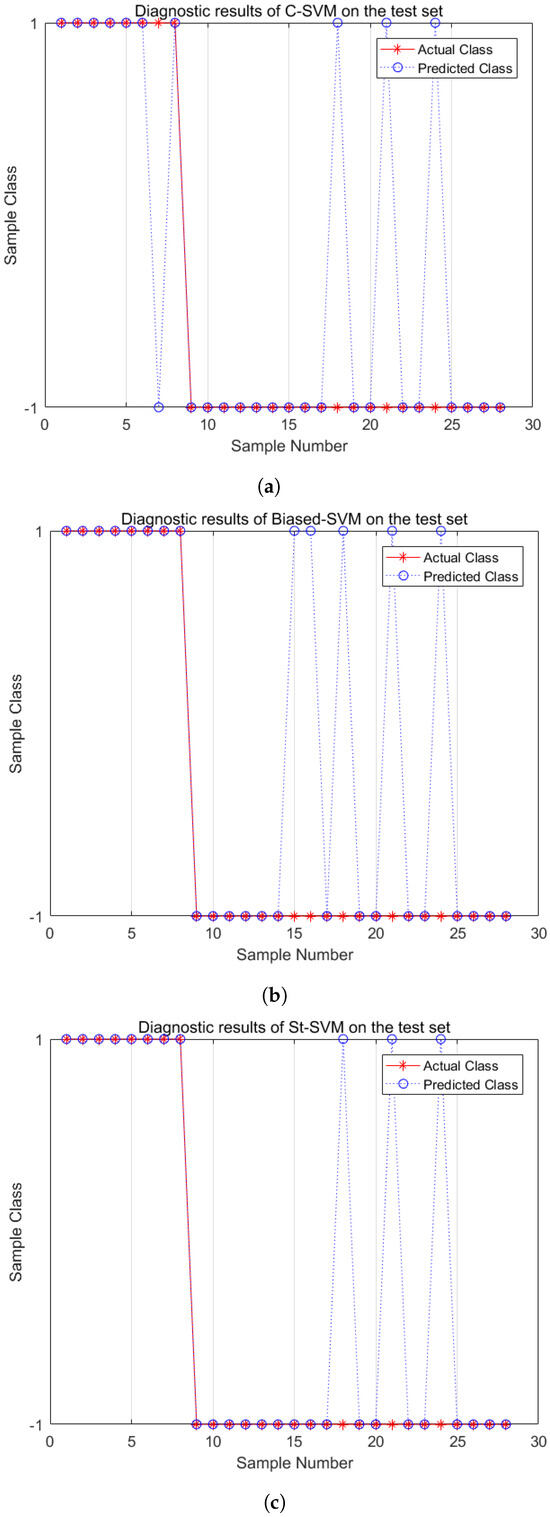
Figure 6.
Fault diagnosis comparisons (IR = 2.5). (a) C-SVM; (b) Biased-SVM; (c) St-SVM.
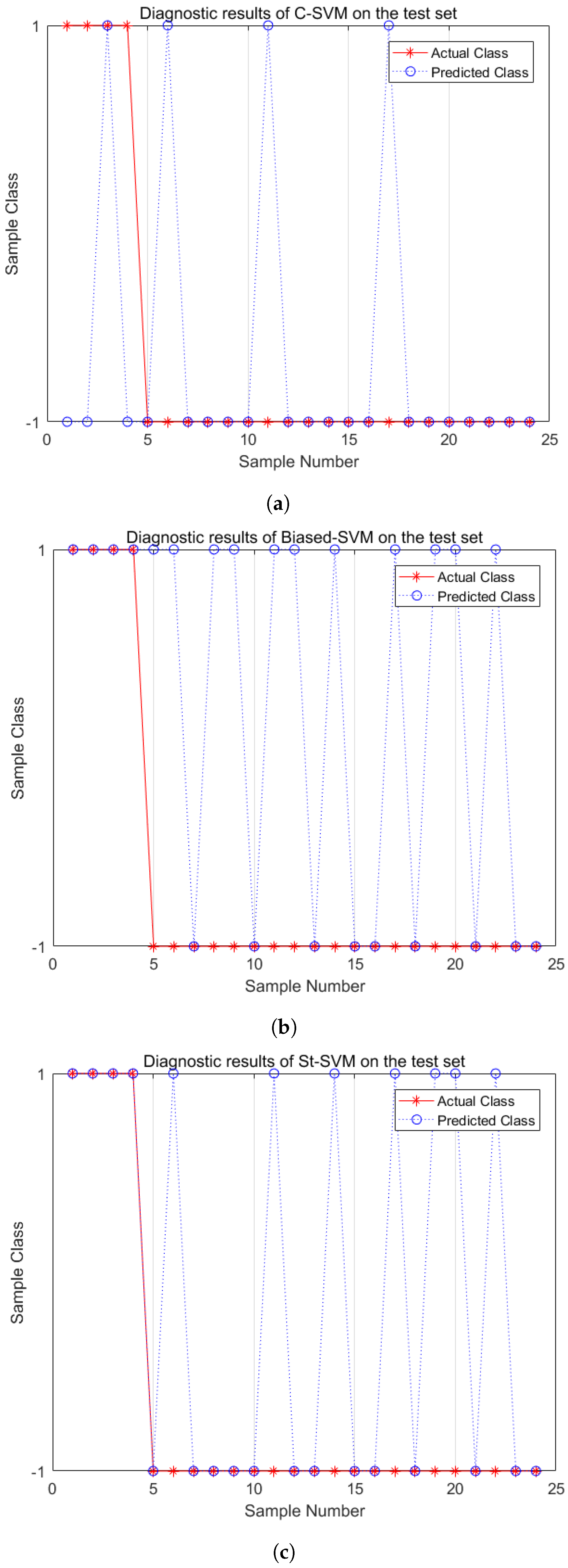
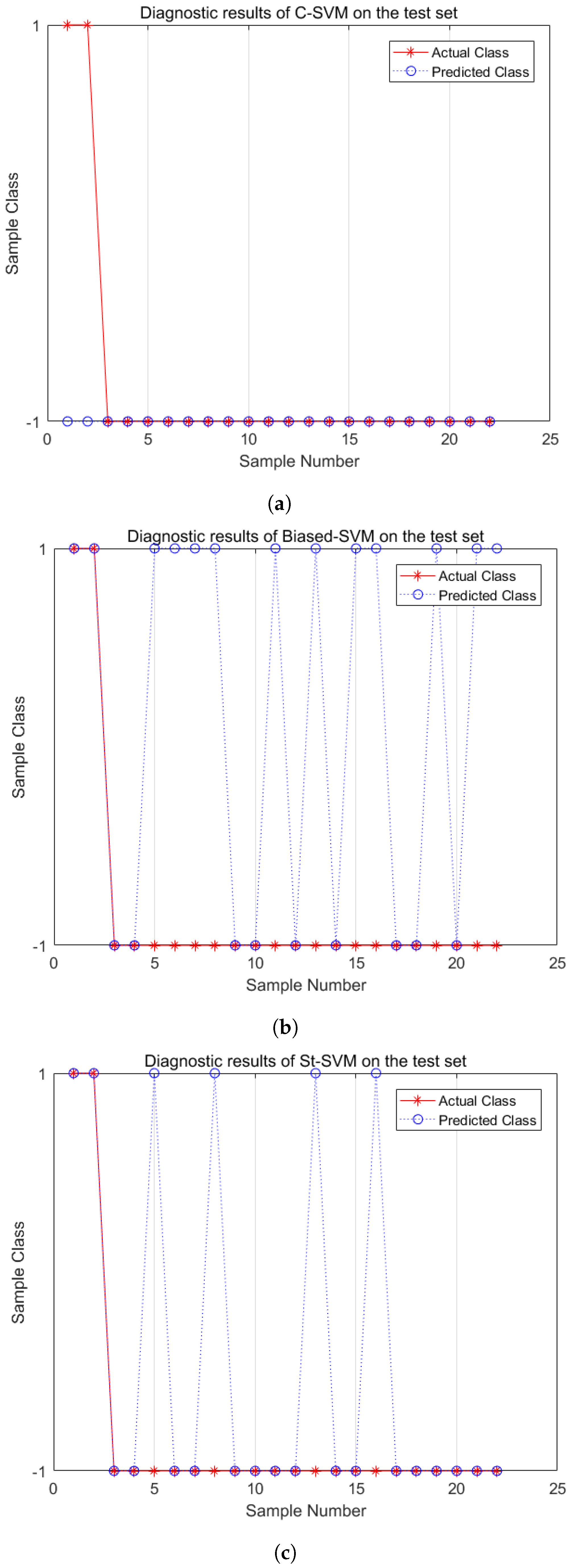
Similarly, Figure 7 and Figure 8 show the fault diagnosis results with IR = 5 and IR = 10. From the diagnosis results of the medium imbalance dataset, the C-SVM shows a significant decrease in the recognition capability of minority-class samples. The Biased-SVM identifies all minority-class samples but misclassifies eleven majority-class samples. The St-SVM improves the recognition rate of minority-class samples while only misclassifying seven majority-class samples. In the experiments of a high imbalance dataset with IR = 10, the C-SVM loses its recognition capability for minority-class samples. The Biased-SVM identifies two minority-class samples while misclassifying eleven majority-class samples. Meanwhile, the St-SVM not only identifies two minority-class samples but also misclassifies only four majority-class samples. In conclusion, the St-SVM demonstrates its superiority in classification performance in fault diagnosis of both medium and high imbalance datasets.
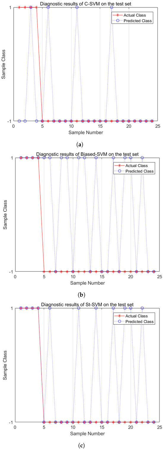
Figure 7.
Fault diagnosis comparisons (IR = 5). (a) C-SVM; (b) Biased-SVM; (c) St-SVM.
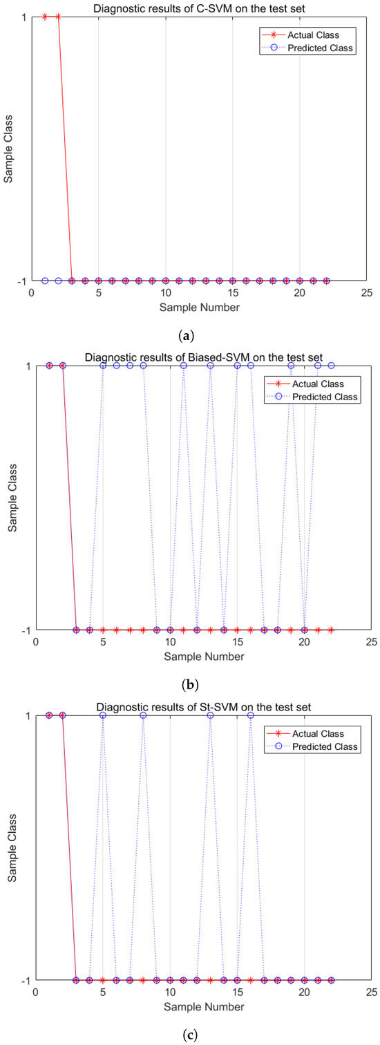
Figure 8.
Fault diagnosis comparisons (IR = 10). (a) C-SVM; (b) Biased-SVM; (c) St-SVM.
Table 2, Table 3 and Table 4 represent the mean classification performance evaluation metrics of C-SVM, Biased-SVM, and St-SVM based on the test set with IR = 2.5, IR = 5 and IR = 10, respectively. 1. The G-mean, a metric for evaluating the classification performance of the conventional SVM, is relatively high when the data imbalance ratio is low, indicating superior diagnostic performance under these conditions. However, as the data imbalance ratio increases, the G-mean metric decreases, reflecting a decline in diagnostic efficiency. 2. The Biased-SVM shows a certain improvement compared to the traditional SVM. Its Sensitivity metric, which measures the ability to correctly identify minority-class samples, is enhanced, demonstrating a stronger capability in recognizing minority-class samples. However, a decrease in the Specificity metric, which reflects the proportion of majority-class samples correctly identified, indicates that it misclassifies more majority-class samples. This trade-off highlights the bias towards the minority-class in the model decision-making process. 3. The St-SVM consistently exhibits higher G-mean values than both the traditional and Biased-SVM, suggesting superior diagnostic performance across all data imbalance ratios. As the dataset imbalance ratio increases, the G-mean remains stable, indicating strong generalization capabilities.
Table 2.
Performance metric (IR = 2.5).
Table 3.
Performance metric (IR = 5).
Table 4.
Performance metric (IR = 10).
5.4. Application on Real-World Imbalanced Fault Datasets of Electric Traction Systems
In order to further verify the effectiveness of the proposed method in practical applications for high-speed train electric traction systems, we applied the method to the Case Western Reserve University (CWRU) bearing dataset [19], which shares similar structural and physical characteristics, and fault modes (including inner race faults, outer race faults, ball faults, and normal conditions) with those of the motor bearings in high-speed train electric traction systems. Therefore, the bearing fault data from CWRU can provide us with valuable information regarding bearing fault detection and diagnosis, contributing to the research on fault analysis and maintenance strategies for electric traction systems. When dealing with the transition from the simulation model to real systems with noise and uncertainties, comprehensive approaches can be employed, including data cleaning, smoothing and filtering techniques, statistical analysis, and dimensionality reduction, as well as machine learning denoising methods. The aforementioned methods can be optimized through preliminary experiments, and data should be monitored in real-time to ensure the model accuracy and reliability in noisy environments. Vibration signals are selected from the SKF6205 bearing model located at the motor drive end in the CWRU bearing dataset, specifically under the conditions of a sampling frequency of 12 kHz and a rotational speed of 1797 revolutions per minute (RPM). Firstly, mean filtering is used for data preprocessing to reduce the interference of noise. Subsequently, due to the limited number of signal samples in the CWRU dataset, data augmentation is performed using a sliding window technique. The sliding window size is set to 500, with an overlap rate of 50%. Finally, the following time-domain features are calculated for each window: standard deviation, mean absolute value, and kurtosis. A highly imbalanced dataset with an IR of 10 is considered, containing 440 samples in total, with 400 samples belonging to the majority class and 40 samples to the minority class. Multiple experiments are conducted and their results are averaged in order to reduce the impact of randomness on the outcomes. The additional experimental results based on real bearing fault data are shown in Figure 9 and Table 5.
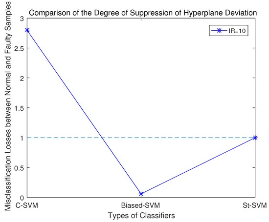
Figure 9.
Comparisons of misclassification losses of different classifiers with the CWRU dataset.
Table 5.
Performance metric (CWRU dataset with IR = 10).
As shown in Figure 9, C-SVM aims to minimize the overall loss during the optimization process, with a unified penalty factor. Consequently, the loss of the minority class is higher than that of the majority class, resulting in a suppression ratio R > 1. On the other hand, Biased-SVM assigns penalty factor weights to the minority class based on the imbalance ratio of the dataset. When dealing with highly imbalanced fault classification problems, the larger weights cause the algorithm to overly focus on minority-class samples, significantly reducing the classification accuracy of the majority-class samples, resulting in poor fault classification performance in further samples. Thus, the loss of the majority-class samples is much larger than that of the minority class, with a suppression ratio R < 1 and close to 0. The proposed St-SVM in this paper assigns different penalty factors to each sample based on the information content, achieving a suppression ratio R = 1, demonstrating excellent suppression ability and superior fault classification performance.
The results in Table 5 further confirm the aforementioned analysis, with the G-mean indicator of St-SVM significantly higher than that of both C-SVM and Biased-SVM, indicating that the proposed method in this paper achieves better performance on real-world imbalanced bearing datasets. Compared with the other two algorithms, St-SVM is more suitable for handling fault diagnosis problems characterized by overlapping and imbalanced datasets in real working conditions. It is capable of assigning different penalty factors based on sample information, which allows it to balance classification accuracy between majority and minority samples, thus improving the overall performance of fault classification.
6. Conclusions
In the context of fault diagnosis for high-speed train electric traction systems, this paper introduces an St-SVM strategy. This approach intelligently modulates the penalization strength in response to the informational content of the samples, thereby efficaciously resolving diagnostic challenges in scenarios where data are imbalanced, a prevalent issue in high-speed trains. Using the TDCS-FIB simulation platform of the CRH2 high-speed train electric traction system, and its three datasets of different IRs, as well as the CWRU bearing fault dataset, as samples, this paper elaborates on the specific design steps, evaluation metrics, and classification performance analyses when incorporating the St-SVM strategy. Experimental results demonstrate that the proposed fault diagnosis scheme consistently ensures equal risk loss for both normal and faulty data, mitigating classification margin shift and accurately identifying minority-class samples. It exhibits outstanding overall performance in addressing imbalanced datasets in high-speed train electric traction systems.
Author Contributions
Conceptualization, Y.W. and T.J.; methodology, T.J. and Y.Z. (Yang Zhou); software, T.J.; validation, Y.W. and T.J.; formal analysis, Y.W.; investigation, T.J.; resources, Y.W.; data curation, Y.W. and T.J.; writing—original draft preparation, T.J.; writing—review and editing, Y.W.; visualization, Y.Z. (Yijin Zhou); supervision, Y.Z. (Yang Zhou); project administration, Y.W.; funding acquisition, Y.W. All authors have read and agreed to the published version of the manuscript.
Funding
This work was supported in part by the National Natural Science Foundation of China under Grants (62173164, 62203192), in part by the 6th regular meeting exchange program (6-3) of the China-North Macedonian Science and Technology Cooperation Committee.
Data Availability Statement
Data are contained within the article.
Conflicts of Interest
The authors declare no conflicts of interest.
Abbreviations
The following abbreviations are used in this manuscript:
| SVM | Support Vector Machine |
| St-SVM | Self-tuning Support Vector Machine |
| IR | Imbalance Ratio |
| CRH | China Railway High-speed |
References
- Cheng, C.; Wang, W.; Chen, H.; Zhang, B.; Shao, J.; Teng, W. Enhanced fault diagnosis using broad learning for traction systems in high-speed trains. IEEE Trans. Power Electron. 2020, 36, 7461–7469. [Google Scholar] [CrossRef]
- Liu, Z.X.; Wang, Z.Y.; Wang, Y.; Ji, Z.C. Optimal zonotopic Kalman filter-based state estimation and fault-diagnosis algorithm for linear discrete-time system with time delay. Int. J. Control Autom. Syst. 2022, 20, 1757–1771. [Google Scholar] [CrossRef]
- Chen, H.; Jiang, B.; Ding, S.X.; Huang, B. Data-driven fault diagnosis for traction systems in high-speed trains: A survey, challenges, and perspectives. IEEE Trans. Intell. Transp. Syst. 2020, 23, 1700–1716. [Google Scholar] [CrossRef]
- Yang, X.; Yang, C.; Yang, C.; Peng, T.; Chen, Z.; Wu, Z.; Gui, W. Transient fault diagnosis for traction control system based on optimal fractional-order method. ISA Trans. 2020, 102, 365–375. [Google Scholar] [CrossRef]
- Wu, Y.; Liu, X.; Wang, Y.L.; Li, Q.; Guo, Z.; Jiang, Y. Improved deep PCA and Kullback–Leibler divergence based incipient fault detection and isolation of high-speed railway traction devices. Sustain. Energy Technol. Assess. 2023, 57, 103208. [Google Scholar] [CrossRef]
- Li, Y.; Li, F.; Lu, C.; Fei, J.; Chang, B. Composite fault diagnosis of traction motor of high-speed train based on support vector machine and sensor. Soft Comput. 2023, 27, 8425–8435. [Google Scholar] [CrossRef]
- Liao, J.; Shi, X.J.; Zhou, S.L.; Xiao, Z.C. Analog circuit fault diagnosis based on local graph embedding weighted-penalty SVM. Trans. China Electrotech. Soc. 2016, 31, 28–35. [Google Scholar]
- Zhang, Y.; Jiang, Y.; Chen, Y.; Zhang, Y. Fault diagnosis of high voltage circuit breaker based on multi-classification relevance vector machine. J. Electr. Eng. Technol. 2020, 15, 413–420. [Google Scholar] [CrossRef]
- Li, Y. Exploring real-time fault detection of high-speed train traction motor based on machine learning and wavelet analysis. Neural Comput. Appl. 2022, 34, 9301–9314. [Google Scholar] [CrossRef]
- Ye, M.; Yan, X.; Jia, M. Rolling bearing fault diagnosis based on VMD-MPE and PSO-SVM. Entropy 2021, 23, 762. [Google Scholar] [CrossRef] [PubMed]
- Li, Y.X.; Chai, Y.; Hu, Y.; Yin, H.P. Review of imbalanced data classification methods. Control. Decis. 2019, 34, 673–688. [Google Scholar] [CrossRef]
- Zhang, T.; Chen, J.; Li, F.; Zhang, K.; Lv, H.; He, S.; Xu, E. Intelligent fault diagnosis of machines with small & imbalanced data: A state-of-the-art review and possible extensions. ISA Trans. 2022, 119, 152–171. [Google Scholar] [PubMed]
- Shi, Q.; Zhang, H. Fault diagnosis of an autonomous vehicle with an improved SVM algorithm subject to unbalanced datasets. IEEE Trans. Ind. Electron. 2020, 68, 6248–6256. [Google Scholar] [CrossRef]
- Viegas, F.; Rocha, L.; Gonçalves, M.; Mourão, F.; Sá, G.; Salles, T.; Andrade, G.; Sandin, I. A genetic programming approach for feature selection in highly dimensional skewed data. Neurocomputing 2018, 273, 554–569. [Google Scholar] [CrossRef]
- Sitompul, O.S.; Nababan, E.B. Biased support vector machine and weighted-SMOTE in handling class imbalance problem. Int. J. Adv. Intell. Inform. 2018, 4, 21–27. [Google Scholar]
- Xu, S.; Chai, H.; Hu, Y.; Huang, D.; Zhang, K.; Chai, Y. Simultaneous Fault Diagnosis of Broken Rotor Bar and Speed Sensor for Traction Motor in High-speed Train. Zidonghua Xuebao 2023, 49, 1214–1227. [Google Scholar]
- Akbani, R.; Kwek, S.; Japkowicz, N. Applying support vector machines to imbalanced datasets. In Machine Learning: ECML 2004: 15th European Conference on Machine Learning, Pisa, Italy, 20–24 September 2004. Proceedings; Springer: Berlin/Heidelberg, Germany, 2004; pp. 39–50. [Google Scholar]
- Sadollah, A.; Sinha, T. Recent Trends in Computational Intelligence; BoD—Books on Demand: Norderstedt, Germany, 2020. [Google Scholar]
- Zhang, X.; Zhao, B.; Lin, Y. Machine learning based bearing fault diagnosis using the case western reserve university data: A review. IEEE Access 2021, 9, 155598–155608. [Google Scholar] [CrossRef]


Disclaimer/Publisher’s Note: The statements, opinions and data contained in all publications are solely those of the individual author(s) and contributor(s) and not of MDPI and/or the editor(s). MDPI and/or the editor(s) disclaim responsibility for any injury to people or property resulting from any ideas, methods, instructions or products referred to in the content. |
© 2024 by the authors. Licensee MDPI, Basel, Switzerland. This article is an open access article distributed under the terms and conditions of the Creative Commons Attribution (CC BY) license (https://creativecommons.org/licenses/by/4.0/).