Abstract
The aim of this study was to determine the most appropriate advanced methods for distinguishing the gait of healthy children (CO) from the gait of children with cerebral palsy (CP) based on electromyography (EMG) parameters and coactivations. An EMG database of 22 children (aged 4–11 years) was used in this study, which included 17 subjects in the CO group and 5 subjects in the CP group. EMG time parameters were calculated for the biceps femoris (BF) and semitendinosus (SE) muscles and coactivations for the rectus femoris (RF)/BF and RF/SE muscle pairs. To obtain a more accurate classification result, data augmentation was performed, and three classification algorithms were used: support vector machine (SVM), k-nearest neighbors (KNNs), and decision tree (DT). The accuracy of the root-mean-square (RMS) parameter and KNN algorithm was 95%, the precision was 94%, the sensitivity was 90%, the F1 score was 92%, and the area under the curve (AUC) score was 98%. The highest classification accuracy based on coactivations was achieved using the KNN algorithm (91–95%). It was determined that the KNN algorithm is the most effective, and muscle coactivation can be used as a reliable parameter in gait classification tasks.
1. Introduction
Electromyography (EMG) is an important tool for investigating muscle functions, providing information on the electrical activity generated by skeletal muscles during contraction and relaxation. EMG is widely used in diagnostics, rehabilitation, sports, ergonomics, etc., analyzing the activity of various muscles during different movements or at rest. One of the areas in which EMG is widely applied is in the analysis of gaits, and the greatest attention is paid to primary muscle activations [1]. However, in order to understand the complex interaction of different muscle groups during gait, it is very important to analyze muscle coactivations together.
Coactivation in a gait refers to the simultaneous activation of muscles that can facilitate movement or provide stability. For example, during walking, the coordinated activity of agonist and antagonist muscles around a joint ensures controlled and balanced movements. This coordination is particularly important for tasks such as maintaining balance during the stance phase or transitioning between different phases of a gait [2,3]. Abnormal coactivation patterns are often associated with various gait disorders and neurological diseases such as, cerebral palsy (CP), stroke, Parkinson’s disease, etc. [4,5] Thus, in order to determine the changes in muscle functions caused by these disorders and to apply therapeutic measures to restore normal walking, it is also necessary to accurately determine muscle coactivation during a gait.
The analysis of gait EMG signals is complicated by several factors. Even during a normal gait, due to the dynamics of the movements, the muscle activation patterns change in different phases of the gait and may be different for each individual. Factors such as the gait speed, terrain, footwear, etc., are also influential [6]. Finally, EMG signals are often contaminated with noise and motion artifacts, so properly selected pre-processing methods are needed to avoid data distortions, such as the duration of the signal, both in terms of amplitude [7,8]. Properly selected signal pre-processing methods allow for the extraction of necessary EMG parameters and for the use of advanced biosignal analysis methods, such as classifications using machine learning. However, there is neither a unified technique on how to prepare the data nor a consensus on what parameters and classification methods to choose in order to obtain the best classification results.
In a quantitative analysis of EMG signals, i.e., before transferring the EMG data to the classifiers, certain steps are taken to ensure the accuracy and utility of the signals. First, pre-processing is performed, which is further divided into two stages: signal segmentation, or cutting, and signal filtering. Segmentation helps reduce data dimensionality and improves classification accuracy, and the window size also affects the classification accuracy [9,10]. Park et al. [10] compared the signal classification accuracy at four different window sizes: 100, 200, 400, and 600 ms. This classification was performed with four different machine learning methods, and it was found that all methods were most efficient when using a window size of 200 ms. In a gait analysis, depending on the task, EMG data can be cut both by certain window sizes [11] and by gait phases [12,13]. Meanwhile, filtering reduces artifacts caused by various factors, such as movements of the sensor at the attachment site, rapid movements of certain body parts, and disturbances of the electrode–skin contact [14]. Low-frequency or bandpass Butterworth filters are often used for filtering the EMG signal of the lower limbs, the order and cut-off frequencies of which are selected according to the specificity of the data and/or after performing a power spectrum analysis of the signal [15,16,17,18]. In the scientific literature, optimal threshold frequencies for EMG bandwidth filtering for conductive EMG sensors are proposed. Generally, the power spectrum of EMG signals ranges from about 20 to 500 Hz [19,20], with low-frequency noise usually occurring in the 0–20 Hz range [21,22]. The recommended cut-off frequency for high-pass filters is 5–30 Hz, and for low-pass filters—400–500 Hz [21,23,24]. After the segmentation and filtering of the EMG signal, further steps such as rectification and normalization are usually performed, and the necessary parameters are extracted.
Extracting parameters from the signal is also of great importance for classification accuracy and performance. Parameters extracted from EMGs can be divided into three main categories: time, frequency, and time–frequency characteristics [25]. Time characteristics include the root mean square (RMS) value, mean absolute value (MAV), zero crossing rate (ZCR), waveform length (WL), and integrated EMG (iEMG). Frequency parameters are commonly used in muscle fatigue assessments and motor unit analyses and include the peak frequency (PK), mean frequency (MNF), and median frequency (MDF) parameters. Yao et al. [12] extracted the RMS, MAV, and WL parameters from an EMG gait data sequence and used them for a gait-phase classification with a support vector machine (SVM). A high gait-phase-classification reliability of 94.89% was achieved with these parameters.
SVM, k-nearest neighbors (KNNs), and decision trees (DTs) are among the most commonly applied supervised learning methods for studying gait data. In the classification of gait EMG data, SVM was used for cases such as CP and control groups [26], people-by-age groups [27], or stance- and swing-phase separations [28], where the classification accuracies were 83.33%, 89%, and 96%, respectively. KNN is also used in gait EMG analyses to compare healthy and pathological gaits [17,29,30,31], recognize foot diseases [32], etc., where the classification accuracy ranges from 67.7% to 99%. It has been observed that SVM performs more accurately than KNNs [17,29]. In addition, the DT method is used for EMG data classification studies. Park et al. [10] used DT, KNN, and SVM algorithms for the recognition of two step phases, stance and swing. The algorithms achieved high accuracies of 91.5%, 90.2%, and 95.2%, respectively. Ramirez-Perez et al. [33] conducted a study on muscle activity recognition using the DT algorithm, and the results obtained allowed the creation of a prosthesis that correctly imitates human movements based on the EMG signal. However, classification methods are currently not extensively tested in attempts to distinguish gait patterns based on coactivations. One of the biggest limitations of using these methods is that the size of the dataset plays a crucial role in the performance of the classification algorithms, especially in the analysis of EMG signals. Larger datasets generally provide better statistical representativeness, better model generalizability, and improved noise control. However, it is not always possible to collect the necessary amount of data or a homogeneous group of patients, especially when it comes to children with CP. Resultantly, state-of-the-art solutions such as data augmentation, transfer learning, or correction can be used to increase the classification accuracy [34,35,36,37].
This study aims to identify the most effective method for accurately classifying subjects into two categories based on gait EMG data. The following tasks will be undertaken: (1) pre-process EMG signals according to their specificity; (2) calculate coactivations and EMG parameters; (3) expand the dataset to enhance the classifier performance; (4) employ different data classification methods; and (5) determine the optimal classification method.
2. Materials and Methods
2.1. Participant and Dataset Descriptions
The database consisted of gait EMG data from 22 subjects (13 girls and 9 boys), who were divided into two groups: healthy (CO) and cerebral palsy (CP). The demographic and anthropometric data of the subjects are presented in Table 1. The CP group consisted of 4 spastic diplegic subjects and 1 spastic hemiplegic subject, with a score of 1 to 3 on the Gross Motor Function Classification System (GMFCS) scale.

Table 1.
Demographic and anthropometric data of subjects (mean ± SD) (n = 22).
To compile the database, the EMG data of five muscles were recorded for both lower limbs using a Delsys Trigno 10 wireless EMG sensor system at 2000 Hz. The muscles monitored were SE, semitendinosus; BF, biceps femoris; MG, medial gastrocnemius head; LG, lateral gastrocnemius head; and RF, rectus femoris. Based on literature recommendations, coactivations were calculated for the muscle pairs of RF with BF and RF with SE, and for extracting temporal parameters, the RF, BF, SE, MG, and LG muscles were selected [13,38]. Gait cycles (from heel contact to heel contact) and their phases for both legs were determined based on measurements of the force plate Bertec (1000 Hz) and the 8-camera optical motion recording system Vicon (100 Hz) guided by the heel and toe marker trajectories. During the study, all subjects walked barefoot at their usual pace for 7 m. The resulting dataset contained a total of 259 measurements: 191 for the CO group (average of 29.1 ± 14.3 gait cycles per subject) and 68 for the CP group (average of 42.2 ± 13.1 gait cycles per subject). The permission of the Regional Bioethics Committee (no. 2020/9-1256-738) and written consent of the children’s parents were obtained for this research.
In this study, the CP group was designated as the positive class, while the CO group was designated as the negative class.
2.2. Study Protocol
To determine the most suitable classification method, this study was conducted in the following main stages (Figure 1): 1. the selection of the optimal pre-processing methods and parameters for EMG data, 2. an extraction of the required EMG signal parameters and calculations of coactivations, 3. data based on available EMG data, 4. the selection of classification methods and their parameters, and 5. an evaluation and a comparison of the results.
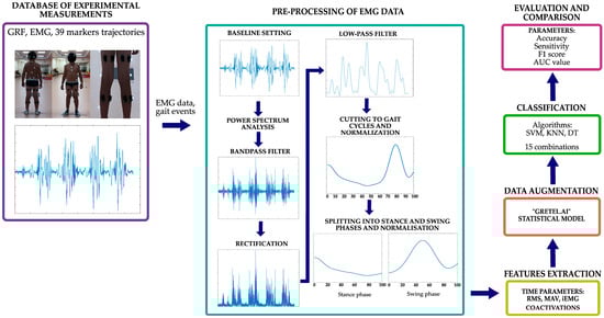
Figure 1.
Scheme of this research.
The software package Matlab_R2023b (The MathWorks, Natick, MA, USA) was used to process the EMG data and perform the classification tasks.
2.2.1. EMG Data Pre-Processing
The EMG sensor data pre-processing included the following steps:
- EMG data baseline determination.
- Filtering with a second-order Butterworth bandpass filter with the lowest (30 Hz) and the highest (500 Hz) cut-off frequency limits being based on the results of a signal power spectrum analysis.
- Full-wave rectification, i.e., the EMG signal is converted from a bipolar to a unipolar form, which facilitates further analysis by removing negative values, and equalization.
- Filtering with a low-pass 5th-order zero-phase Butterworth filter with a cut-off frequency of 6 Hz.
- Signal cutting to gait cycles from heel contact to heel contact based on the camera system and force plate data and performing normalization at a 0–100% gait cycle.
- For the calculations of coactivations, the gait cycle was divided into stance and swing phases in a 60:40 ratio. Then, the signal was again normalized by duration, i.e., 100% of the stance and 100% of the swing phase, and by RMS, i.e., the EMG signal was then normalized by dividing each data point by the RMS value.
2.2.2. Feature Extraction of EMG Signals
The following time parameters were extracted from pre-processed data: the RMS (root mean square), MAV (mean absolute value), and iEMG (integrated EMG). For coactivation calculations, the RMS was further standardized using MATLAB’s “zscore” function. These parameters were selected based on their effectiveness and frequent use in the literature. The mathematical expressions of these parameters were derived from previous studies [39]. The obtained values were standardized to avoid data scatters that could distort the classification accuracy.
After generating the RMS envelope, the coactivation indexes were calculated according to the following formulas [13]:
Coactivation was calculated based on the agonist/antagonist role of the muscles in the stance and swing phases, i.e., coactivations were calculated separately for each phase. Based on a literature analysis of coactivation calculations and muscle activations during gaits, the RF muscle was considered antagonist during the swing phase, while the BF and ST muscles were considered antagonists during the stance phase [40]. In Formula (1) (CoA1), the antagonist activity is normalized to the mean total muscle activity and multiplied by two to account for the agonist activity. Formula (2) (CoA2) compares the activity of the antagonist only with the activity of the agonist. Theoretically, a coactivation index of 100% indicates equal agonist and antagonist muscle activity, while 0% represents only agonist activation. The calculated coactivation values were log-transformed to stabilize any variance and make the distribution of data points more normal, making data more suitable for classification tasks.
2.2.3. Data Augmentation
Since the available set of measured EMG data is too small for the reliable performance of classification tasks, we chose to perform a data synthesis. The “Gretel.ai” statistical model, which supports high volumes of tabular data generation with “Amplify”, was chosen for this purpose. This model can generate a large amount of reliable synthetic data simulating real data. After the data synthesis, each dataset to be classified consisted of 100 variables with 2000 observations per variable for both the CP and CO class. This dataset size was chosen as optimal for several reasons:
- A larger amount of data requires more computer resources, capabilities, and time.
- When synthesizing a larger amount of data, there is a risk that the deviation from the real measured data will be greater, so the goal is to keep as much real data in the set as possible.
2.2.4. Classification
To achieve optimal classification for distinguishing between healthy (CO) and cerebral palsy (CP) groups, three algorithms were employed: support vector machines (SVMs), k-nearest neighbors (KNNs), and decision trees (DTs). First of all, each algorithm was tested with five parameters, RMS, CoA1, CoA2, MAV, and iEMG, resulting in a total of 15 different combinations. The parameters that led to the best classification results were also determined.
Subsequently, in this study, the performance of the following three classifiers in various feature combinations was analyzed: CoA1+RMS, CoA1+MAV, CoA1+iEMG, CoA2+RMS, CoA2+MAV, CoA2+iEMG, RMS+MAV, RMS+iEMG, CoA1+RMS+MAV, CoA1. +RMS+iEMG, CoA1+MAV+iEMG, CoA2+RMS+MAV, CoA2+RMS+iEMG, and CoA2+MAV+iEMG. Since this study heavily focuses on determining the classification efficiency of the coactivation parameter, coactivations were included in all 14 combinations.
To find the most optimal parameters for the SVM, KNN, and DT algorithms, the following main steps were performed:
- Dataset preparation: The entire dataset is processed and divided into training, validation, and testing sets. The sets are divided into 80%, 10%, and 10% parts, respectively.
- The data are prepared for validation using a k-fold cross-validation. A value of k = 10 was chosen, knowing that higher values are recommended when the dataset is larger. The cross-validation used a stratified distribution of the data to ensure that each validation stratum contained equal amounts of data from both classes, thus achieving more reliable results.
- Finding the best parameters: For the SVM algorithm, it is important to choose the best combination of the C parameter and kernel scale (S) by testing the algorithm with different combinations of these parameters. The C parameter is a regularization parameter that controls the trade-off between low training data errors and reduces the model complexity to avoid overfitting. The S parameter affects the width of the Gaussian function used in the kernel. A smaller scale results in a narrower kernel, making the decision boundary more complex, while a larger scale results in a smoother decision boundary. The SVM algorithm was tested with the following values: C = {0.01, 0.03, 0.1, 0.3, 1, 3, 10, 30} and S = {0.01, 0.03, 0.1, 0.3, 1, 3, 10, 30}. Different kernel functions were also tested with all values: Gaussian, quadratic, and cubic.
- For the KNN algorithm, it is important to choose the K parameter correctly, so the following values were tested in this work: K = {1, 2, 3, 4, …., 15}. Two different methods of measuring the distance between neighbors (distance metric) were tested: cosine and L1. We randomly selected one of the tied classes.
- Two parameters are important for the DT algorithm—the maximum number of splits (P) and the split criterion. The following P values were tested in this study: {2, 4, 8, 16, 32, 64}. All values were tested based on two-split criteria—the Gini index and maximum variance reduction (MVR). The Gini index quantifies how often a randomly chosen element from the set would be incorrectly labeled if it were randomly labeled according to the distribution of labels in the node. And MVR is a criterion used to split nodes in decision trees, and it chooses the split to create the most homogeneous nodes possible. The Gini index was employed as the splitting criterion in our decision tree model, specifically utilizing the CART (Classification and Regression Trees) algorithm.
2.2.5. Methods of Evaluation and Comparison of Results
Each algorithm was evaluated according to accuracy, precision (positive predictive value, PPV); sensitivity; specificity; the negative predictive value (NPV); the F1 score; and the area under curve (AUC) score. Precision was calculated as the true positive (TP) divided by the sum of the TP and false positive (FP) [41]:
The aim was to obtain the highest possible precision value. However, it was important that this value was not significantly higher or lower than the confidence value, as this would indicate weaknesses in the data processing, the algorithm parameters chosen, or the dataset. A precision value greater than confidence (>20%) indicates that the algorithm is better at classifying and recognizing the negative class, so the more similar these two values are, the better the algorithm is at recognizing both the negative and positive classes. A difference in values of no more than 10% is considered normal and expected.
Sensitivity shows how well the positive class was detected and was calculated by dividing the TP by the sum of the TP and false negative (FN) [41]:
Specificity describes the maximum negative likelihood ratio (NLR) from a true negative prediction to actual negatives and was calculated by dividing the true negative (TN) by the sum of the TN and FP [41]:
NPV indicates the ratio of negative predictions to all actual negative predictions and shows how many negative test results are true negatives [41]:
Precision and sensitivity are described by a single criterion, called the F1 score. The following criterion was calculated [42]:
The higher the value of F1, the better the balance of the algorithm in recognizing positive and negative data classes. A low score may indicate low sensitivity and precision or a low status of only one of these parameters. The F1 score provides a better assessment of the overall performance of the algorithm than just the assessment of precision or sensitivity. The F1 score can also be compared to confidence, since the confidence score can be deceptively good, even in an unbalanced dataset where one class is much larger than the other. However, in such a case, the F1 score would be lower, which would suggest that the algorithm is not as efficient as it would appear from an analysis of reliability alone.
To evaluate the algorithms, the areas under the receiver operating characteristic (ROC) curves, area under the curves (AUCs)—showing the ratio of sensitivity and specificity of the classifier—were used. The closer the AUC value is to unity, the better the overall performance of the algorithm. Comparing the AUC values allows us to choose the model that is able to distinguish the classes the best.
3. Results
Firstly, data augmentation was performed for the measured EMG database. “Gretel.ai” divides the obtained results into five categories: excellent, good, moderate, poor, and very poor (Figure 2). These categories allow us to decide on the suitability of the data for use in classification tasks. Excellent and good categories are considered suitable for using data for machine learning tasks. Synthesizing the available datasets resulted in the average of a 75% synthetic data quality, which belongs to the “good” category. Thus, given the resulting synthetic data provided by the program, this method can be used for classification tasks. Data augmentation techniques, if not carefully applied, can potentially lead to the overestimation of performance by artificially inflating the dataset. However, many studies have shown that well-designed augmentation strategies improve model generalizations and do not necessarily lead to misleadingly high performance metrics [43,44,45].
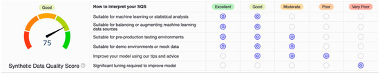
Figure 2.
“Gretel.ai” data quality report.
Table 2 below shows the augmentation results. The augmented data were then used as the input to classifiers. The augmented input for the classifiers consisted of EMG signals categorized into two classes: CO and CP. For each patient, the EMG data were recorded from five muscles in each leg, resulting in a total of 10 features. These features include the root-mean-square (RMS) values, mean absolute value (MAV), integrated EMG (iEMG), and coactivation indexes (CoA1 and CoA2) calculated from the EMG signals. Each feature is input in the classifier separately, but each file contains 10 columns (1 for each muscle in both legs) per patient and 2000 rows, where each row corresponds to an individual observation of these features, providing a comprehensive representation of the muscle activity for both legs.
Table 2.
Dataset size after augmentation.
In this study, the accuracy, precision, sensitivity, F1 score, and AUC score of the algorithms were evaluated in the classification of three time parameters extracted from EMG gait data and coactivations into two classes of subjects. Figure 3 represents the values of all evaluation parameters.
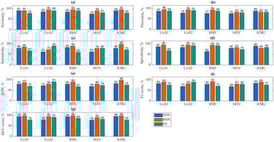
Figure 3.
Results of the algorithms’ accuracy (a), precision (b), sensitivity (c), specificity (d), NPV (e), F1 score (f), and AUC score (g).
Based on graphically presented accuracy values (Figure 3a), the KNN method consistently achieved the highest accuracy across all classified parameters, averaging 93.31%. Specifically, the CoA2+KNN combination showed the highest accuracy at 95.24%. In contrast, the SVM and DT methods performed less effectively, averaging an accuracy of 85.40% and 83.98%, respectively.
The accuracy results indicate that for data classified using the CoA1 formula, both the KNN and SVM algorithms performed well, with DTs lagging behind at 78.26%. SVM showed a slight improvement (+5.59%) when using CoA1, whereas DTs improved significantly (+12.22%) with CoA2. These differences are attributed to variations in calculated values from different formulas, which can greatly impact decision tree classifications. The following results are with regards to specific parameters. (1) The RMS parameter was the most accurately classified by KNN (95%), with SVM and DT also performing reasonably well at 85% and 90.17%, respectively. (2) The MAV parameter had the lowest classification accuracy overall, with KNN achieving the highest accuracy of 90%. SVM performed poorest in classifying MAV compared to other parameters and algorithms. (3) The iEMG parameter was most reliably classified by KNN (95%) but least effectively by DT (80%).
The best precision (Figure 3b) was obtained by CoA1+KNN and the poorest by MAV+SVM. It was found that the classification precision results of the KNN algorithm are the best of all algorithms but were, on average, 3.3% worse than the accuracy results.
Based on Figure 3c, iEMG+KNN achieved the highest sensitivity, indicating a strong recognition of the positive class (CO). However, its precision was lower at 83%. This suggests that while this algorithm identifies positive instances well, there may be some false positives.
When evaluating the specificity (Figure 3d) and NPV results (Figure 3e), we can state that the KNN algorithm is the most reliable model for both specificity (96%) and NPV (iEMG+KNN, 98%), indicating strong performance in correctly identifying negatives and making accurate negative predictions.
Conversely, RMS+DT had the lowest sensitivity at 60%, but it exhibited higher precision at 88%. This indicates that this algorithm performs better at recognizing the negative class (not S), with fewer false positives. Figure 3f presents the F1 scores, which are comprehensive metrics combining precision and sensitivity, making them easier for evaluation.
The RMS+KNN algorithm achieved the highest F1 score, correlating with its high accuracy of 95%. This indicates this algorithm’s balanced performance in recognizing both negative and positive classes, resulting in a high overall accuracy. Other algorithms that also performed well include CoA1+KNN, CoA2+DT, and iEMG+KNN, which obtained high F1 scores, reflecting their effective performance across both classes. Conversely, the algorithms MAV+SVM, CoA2+SVM, and RMS+DT achieved the lowest F1 scores, ranging from 69% to 71%. These scores suggest these algorithms may struggle with either precision, sensitivity, or both, leading to lower overall performance.
In Figure 3g, the AUC (area under the curve) values provide a comprehensive measure of algorithm performance, which is crucial for an accurate evaluation and comparison. CoA1+KNN, RMS+KNN, and iEMG+KNN achieved the highest AUC scores at 98%. This indicates excellent overall performance in distinguishing between classes, with high rates of true positives and true negatives. SVM with similar parameters also demonstrated high AUC values, suggesting robust performance comparable to KNN in these cases. Vice versa, DT with these parameters showed the lowest AUC values. This implies that DTs may struggle more in accurately classifying data compared with KNNs and SVMs in this context.
To analyze and compare which parameters of the SVM classifiers led to the best results based on accuracy, precision, sensitivity, F1 score, and AUCs, Table 3 summarizes these findings.
Table 3.
SVM parameters that led to the best classification results.
After evaluating various kernel functions and parameters in our study, notable trends emerged across different classification parameters. Specifically, the cubic kernel function with a C parameter of 1 consistently delivered optimal results for the CoA1, MAV, and iEMG parameters. Conversely, the Gaussian function with a kernel scale of 30 and a C parameter of 10 proved most effective for the CoA2 and RMS parameters. Across all evaluations, the cubic kernel function with C parameter 1 stood out with the highest accuracy (91.30%) and AUC score (95%), indicating its superior performance. In contrast, the quadratic kernel function demonstrated inadequate reliability across all parameters. For a detailed breakdown of the best performing KNN parameters, please refer to Table 4.
Table 4.
KNN parameters that led to the best classification results.
It can be seen that the most efficient method of measuring the distance between neighbors for these data was cosine, when K = 10. The L1 measurement method resulted in the worst (90%) classification accuracy. Table 5 shows the best performing DT parameters.
Table 5.
DT parameters that led to the best classification results.
It was found that the MVR criterion led to the best classification results more often, but the number of division Ps varies depending on the parameter being classified. Overall, the best DT classification accuracy was determined by the Gini division criterion, with the number of divisions being 16, and the MVR division criterion, with the number of divisions being 32.
Summarizing all the obtained results, it can be said that the best accuracy was obtained with the CoA2+KNN algorithm (95.24%). However, taking into account all evaluation criteria, one algorithm, which gave the best results, stood out: RMS+KNN with the cosine measurement method between neighbors and the number of neighbors K = 10, obtained an accuracy of 95%.
Table 6 shows the classification results for various parameter combinations.
Table 6.
Results of combined parameters (values are in percentages).
The SVM classifier demonstrated strong performance across several metrics, particularly in terms of precision and specificity. In combinations involving iEMG, SVM achieved high precision (88.0% for CoA1+iEMG) and specificity (88.5% for CoA1+iEMG), indicating its effectiveness in correctly identifying true positives and excluding false positives. The SVM’s accuracy was also notable, particularly in the CoA1+iEMG combination, where it reached 90.7%. However, SVM’s performance was less consistent in combinations involving MAV, where the accuracy dropped to 83.2% for CoA1+MAV. Despite this, SVM maintained a solid F1 score across most combinations, reflecting a balanced performance between precision and sensitivity. The AUC scores for SVM were also strong, particularly in combinations involving iEMG (e.g., 95.5% for CoA1+iEMG), suggesting a robust overall classification ability. However, SVM showed moderate sensitivity, especially in combinations with RMS and MAV, indicating that it might miss some true positives compared to KNNs.
KNN consistently outperformed the other classifiers across almost all metrics and feature combinations, emerging as the most reliable classifier in this study. KNN’s accuracy was the highest among the classifiers, particularly in combinations involving iEMG (e.g., 95.1% for CoA2+iEMG and CoA1+iEMG). This high accuracy was complemented by excellent precision, especially in combinations involving RMS (e.g., 94.5% for CoA2+RMS) and iEMG (e.g., 94.0% for CoA1+RMS), highlighting KNN’s capability in minimizing false positives. Furthermore, KNN excelled in sensitivity, often surpassing 90% in combinations involving RMS and iEMG, indicating its strong ability to detect true positives. KNN also maintained high specificity across most combinations, particularly with RMS (e.g., 94.0% for CoA1+RMS), reflecting its efficiency in correctly identifying true negatives. The AUC scores for KNN were consistently the highest across all classifiers, reaching up to 98.0% for combinations like CoA1+RMS, demonstrating its superior ability to distinguish between classes. Overall, the performance of KNN was exceptional, particularly in combinations involving iEMG and RMS, making it the most robust and reliable classifier in this study.
The performance of the DT classifier was more variable compared to SVM and KNN, with notable fluctuations across different combinations. While DT achieved relatively high accuracy in some cases, such as CoA2+RMS (90.4%) and CoA2+RMS+MAV (87.2%), its performance was generally lower than that of KNN and SVM. The DT’s precision varied significantly, particularly in combinations involving MAV (e.g., 83.7% for CoA1+MAV), suggesting a higher likelihood of false positives in these scenarios. Sensitivity for DT was also inconsistent, with strong results in some combinations (e.g., 90.0% for CoA2+RMS) but significantly lower ones in others (e.g., 66.0% for RMS+iEMG), indicating that DTs may miss a considerable number of true positives in certain contexts. Specificity, while high in certain cases (e.g., 92.0% for CoA2+RMS), was generally less consistent compared to KNN, particularly in combinations involving MAV and RMS. DT also showed lower F1 scores in certain combinations, such as CoA1+RMS (76.5%), reflecting an imbalance between precision and sensitivity. The AUC scores for DT were similarly variable, with the highest scores observed in combinations like CoA2+RMS+MAV (88.0%), but generally lower than KNN across most combinations. These findings suggest that while DTs can perform well in certain scenarios, particularly where interpretability is crucial, their overall performance is less reliable and more context-dependent than that of KNNs and SVMs.
In summary, KNN outperformed the other classifiers in parameter combination classifications, achieving the highest accuracy, precision, and AUC scores, especially for iEMG and RMS features. SVM showed high accuracy and specificity but was less consistent in sensitivity. The performance of DT was more variable, being better in some combinations, but generally inferior compared to KNN and SVM. Overall, KNN was the most reliable classifier.
4. Discussion
The aims of this study were to find the most effective algorithm which allows for the accurate classification of subjects into two categories and to determine whether coactivations are suitable parameters for distinguishing gait patterns. In the case of this study, the effectiveness was defined by several evaluation criteria (accuracy, precision, sensitivity, the F1 score, and the AUC score), which are reflected in the results. As already discussed, the best reliability results were obtained by the RMS+KNN algorithm. This algorithm was singled out considering not only its value of accuracy but also by comparing the scores of sensitivities, precision, F1, and AUC, which allowed for a reliable selection of the best algorithm.
Compared to studies reported in the literature, better results were obtained than Fricke et al.’s [17] results, where the KNN algorithm achieved a reliability of 48.7% for a similar classification task. Their study also classified gait into two classes, control and atypical, and used the same temporal characteristics (RMS and iEMG). Despite the similarities, the SVM results obtained by this study was also higher (91.30%) than that obtained by Fricke et al. [17] (67.6%). The results obtained in our study are also better compared to those of Eltanani et al. [31] (67.7%). This shows that the data processing performed in this study, including filtering, standardization, and parameter calculation, is suitable for reliable data classification. Park et al. [10] used DT, KNN, and SVM algorithms to recognize two stride phases, stance and bridge, from a muscle synergy parameter derived from EMG data. The algorithms achieved a high reliability of 91.5%, 90.2%, and 95.2%, respectively. In Park et al.’s [10] study, the results of DT are higher than those obtained in this study, but the results of SVM and KNN are similar. In our study, the poorer result could have been determined by the inappropriate data processing method chosen for the DT algorithm or the insufficiently optimal parameters chosen for classification. The low DT results indicate an area that could be explored in further research to efficiently classify gaits with decision trees.
Coactivation was calculated using two different formulas based on Gagnat et al.’s [13] study and used for gait classification. There are no studies in the literature that use coactivation values to classify gaits into typical and pathological, so the results obtained cannot be compared with other studies. However, the obtained classification accuracy values of the CoA1+SVM, CoA1+KNN, CoA2+SVM, and CoA2+KNN algorithms show that coactivation can be effectively used to distinguish between typical and CP gaits. Also, two different formulas were used to calculate coactivation, with which different classification results were obtained. Such results are in agreement with Gagnat et al.’s [13] study, which concluded that both formulations resulted in different muscle coactivation patterns when comparing healthy and CP patients. The values calculated by the first formula gave the same classification results with the SVM and KNN algorithms but lower ones with DT. Meanwhile, the values calculated by the second formula gave the worst result with SVM but a good one with KNN and DT. The different results obtained with SVM and DT may have been due to the different methods used to calculate coactivation. It is also known that the DT method is sensitive to changes in the data, and even small changes can lead to large differences in the resulting classification values [46]. Thus, it can be said that the CoA2 values were more suitable for decision tree classification than those of CoA1. As research on coactivation efficiency classification tasks continues, other formulas for calculating coactivations should be tested. Also, the gait cycle should be divided into more phases, since the gait of CP patients under study is unstable. Thus, having more step phases would potentially yield more accurate coactivation values and, at the same time, potentially even more efficient classification algorithms.
The obtained results were evaluated according to accuracy, precision, sensitivity, and the F1 score and AUC score. The obtained values were also compared with each other, since it is known that large (>20%) differences between, for example, sensitivity and reliability mean that the algorithm is not able to properly distinguish between positive and negative classes. A difference greater than 20% between accuracy and sensitivity values in the obtained results was observed in the CoA2+SVM, CoA2+KNN, and RMS+DT algorithms. Although the datasets used were balanced and this could not determine a big difference, in the future, it would be worthwhile to try other coactivation calculation methods for the SVM and KNN algorithms and to isolate other parameters for the DT algorithm. The low sensitivity of the algorithms may also be due to the fact that the CP gait of children is classified, which is unstable, and the values of coactivation or other parameters can vary significantly between patients, i.e., due to different forms of CP, levels of damage, etc. In future studies, by dividing the gait cycle into more phases, the obtained coactivation and RMS values would be more accurate, as they would reflect the step in more detail. The literature also consists of studies that observed a large difference between sensitivity and accuracy, where sensitivity is much lower. One such study is Fricke et al. [17], where low sensitivity values (45.8% and 25%) were found, resulting in a low accuracy (32.4% and 51.4%) with the SVM and KNN algorithms. Because the available dataset was small (total of 259 measurements), it was not sufficient to obtain classification results that could be reliably used in future studies. Synthetic data were used to increase the dataset. Although it is noted in the literature that data augmentation methods are currently being studied and are sufficiently accurate [35,36,37], synthetic data based on real measured EMG data may have small deviations that are not characteristic of the measured data [47]. These deviations could also account for the results obtained. However, in the situation of this study, where it was not possible to measure additional data, the synthetic data were a good alternative to understand the influence of the selected parameters on the classification task and to test the validity of the synthetic data. In the future, studies should be conducted using the same methods with a larger set of measured data.
Following this study, several observations and suggestions can be made for researchers who intend to validate the findings of this study by conducting a similar study. In particular, coactivation is an effective parameter for gait data classification, and in order to obtain better classification results, it is recommended to divide the gait cycle into more stride subphases and calculate coactivations for each obtained subphase. Also, results may vary when cutting gait phases according to individual measured gait events. Of course, it is recommended to take into account the specific pathology of the subjects and the type of gait, since the accuracy of the coactivation values depends on it. In this study, three algorithms were selected for classification: SVM, KNN, and DT. It is recommended to try the same data processing methods for the classification of gait data using neural networks, since these algorithms in the literature are also effective for classification. This study used synthetic data due to the small available dataset. It is important to take into account that their quality is as high as possible and sufficient for machine learning, since the efficiency of the algorithm depends on it. It is recommended to test the algorithm trained on synthetic EMG data with measured EMG data.
5. Conclusions
This study employed classification algorithms to distinguish pathological gaits in children using EMG time parameters and coactivations. By advancing the methodology for gait classification and providing new insights into parameter effectiveness, this paper contributes to the ongoing development of more accurate and reliable diagnostic tools in the field of cerebral palsy research. Evaluating classification algorithms based on accuracy, precision, sensitivity, the F1 score, and the AUC score revealed that the KNN algorithm stands out as the most effective. Muscle coactivation emerged as a reliable parameter for classifying cerebral palsy (CP) gait abnormalities. Different methods of calculating coactivations influenced the accuracy of the algorithm: SVM performed best with CoA1 (91.30%); DT with CoA2 (90.48%); and KNN with CoA1 (91.30%), CoA2 (95.24%), CoA2+iEMG, and CoA1+iEMG (95.1%). Implementing this technique could streamline gait analyses for healthcare professionals, aiding in the accurate selection of treatment and rehabilitation strategies tailored to children’s needs, thereby enhancing their overall health and well-being.
Author Contributions
Conceptualization, K.D. and J.Z.; methodology, J.Z. and K.L.; software, K.L.; validation, K.L., J.Z. and K.D.; formal analysis, K.D.; investigation, J.Z. and K.L.; resources, J.Z. and K.L.; data curation, J.Z.; writing—original draft preparation, K.L. and J.Z.; writing—review and editing, K.D. and J.Z.; visualization, J.Z.; supervision, K.D. All authors have read and agreed to the published version of the manuscript.
Funding
This research received no external funding.
Informed Consent Statement
Parental consent and child assent was obtained for all subjects involved in this study.
Data Availability Statement
Data are unavailable due to privacy or ethical restrictions.
Acknowledgments
We would like to thank the medical team of the Children’s Hospital at the Vilnius University Hospital Santaros Klinikos who participated in the collection of the research data.
Conflicts of Interest
The authors declare no conflicts of interest.
References
- Guo, Y.; Gravina, R.; Gu, X.; Fortino, G.; Yang, G.-Z. EMG-based Abnormal Gait Detection and Recognition. In Proceedings of the 2020 IEEE International Conference on Human-Machine Systems, ICHMS 2020, Rome, Italy, 7–9 September 2020. [Google Scholar] [CrossRef]
- Smith, S.; Rush, J.; Glaviano, N.R.; Murray, A.; Bazett-Jones, D.; Bouillon, L.; Blalckburn, T.; Norte, G. Sex influences the relationship between hamstrings-to-quadriceps strength imbalance and co-activation during walking gait. Gait Posture 2021, 88, 138–145. [Google Scholar] [CrossRef] [PubMed]
- Akl, A.R.; Conceição, F.; Richards, J. An exploration of muscle co-activation during different walking speeds and the association with lower limb joint stiffness. J. Biomech. 2023, 157, 111715. [Google Scholar] [CrossRef] [PubMed]
- Ippersiel, P.; Dussault-Picard, C.; Mohammadyari, S.G.; De Carvalho, G.B.; Chandran, V.D.; Pal, S.; Dixon, P.C. Muscle coactivation during gait in children with and without cerebral palsy. Gait Posture 2024, 108, 110–116. [Google Scholar] [CrossRef]
- Gharehbolagh, S.M.; Dussault-Picard, C.; Arvisais, D.; Dixon, P.C. Muscle co-contraction and co-activation in cerebral palsy during gait: A scoping review. Gait Posture 2023, 105, 6–16. [Google Scholar] [CrossRef] [PubMed]
- Agostini, V.; Ghislieri, M.; Rosati, S.; Balestra, G.; Knaflitz, M. Surface Electromyography Applied to Gait Analysis: How to Improve Its Impact in Clinics? Front. Neurol. 2020, 11, 561815. [Google Scholar] [CrossRef]
- Reeves, J.; Starbuck, C.; Nester, C. EMG gait data from indwelling electrodes is attenuated over time and changes independent of any experimental effect. J. Electromyogr. Kinesiol. 2020, 54, 102461. [Google Scholar] [CrossRef]
- Schlink, B.R.; Nordin, A.D.; Ferris, D.P. Comparison of signal processing methods for reducing motion artifacts in high-density electromyography during human locomotion. IEEE Open J. Eng. Med. Biol. 2020, 1, 156–185. [Google Scholar] [CrossRef]
- Gao, S.; Gong, J.; Chen, B.; Zhang, B.; Luo, F.; Yerabakan, M.O.; Pan, Y.; Hu, B. Use of Advanced Materials and Artificial Intelligence in Electromyography Signal Detection and Interpretation. Adv. Intell. Syst. 2022, 4, 2200063. [Google Scholar] [CrossRef]
- Park, H.; Han, S.; Sung, J.; Hwang, S.; Youn, I.; Kim, S.-J. Classification of gait phases based on a machine learning approach using muscle synergy. Front. Hum. Neurosci. 2023, 17, 1201935. [Google Scholar] [CrossRef]
- Qin, P.; Shi, X. Evaluation of Feature Extraction and Classification for Lower Limb Motion Based on sEMG Signal. Entropy 2020, 22, 852. [Google Scholar] [CrossRef]
- Yao, T.; Gao, F.; Zhang, Q.; Ma, Y. Multi-feature gait recognition with DNN based on sEMG signals. Math. Biosci. Eng. 2021, 18, 3521–3542. [Google Scholar] [CrossRef] [PubMed]
- Gagnat, Y.; Brændvik, S.M.; Roeleveld, K. Surface Electromyography Normalization Affects the Interpretation of Muscle Activity and Coactivation in Children with Cerebral Palsy during Walking. Front. Neurol. 2020, 11, 202. [Google Scholar] [CrossRef] [PubMed]
- Martinek, R.; Ladrova, M.; Sidikova, M.; Jaros, R.; Behbehani, K.; Kahankova, R.; Kawala-Sterniuk, A. Advanced Bioelectrical Signal Processing Methods: Past, Present, and Future Approach—Part III: Other Biosignals. Sensors 2021, 21, 6064. [Google Scholar] [CrossRef]
- Nadzri, A.A.B.A.; Ahmad, S.A.; Marhaban, M.H.; Jaafar, H. Characterization of surface electromyography using time domain features for determining hand motion and stages of contraction. Australas. Phys. Eng. Sci. Med. 2014, 37, 133–137. [Google Scholar] [CrossRef]
- Daunoraviciene, K.; Ziziene, J.; Pauk, J.; Juskeniene, G.; Raistenskis, J. EMG Based Analysis of Gait Symmetry in Healthy Children. Sensors 2021, 21, 5983. [Google Scholar] [CrossRef]
- Fricke, C.; Alizadeh, J.; Zakhary, N.; Woost, T.B.; Bogdan, M.; Classen, J. Evaluation of Three Machine Learning Algorithms for the Automatic Classification of EMG Patterns in Gait Disorders. Front. Neurol. 2021, 12, 666458. [Google Scholar] [CrossRef] [PubMed]
- Al-Angari, H.M.; Kanitz, G.; Tarantino, S.; Cipriani, C. Distance and mutual information methods for EMG feature and channel subset selection for classification of hand movements. Biomed. Signal. Process. Control 2016, 27, 24–31. [Google Scholar] [CrossRef]
- Go, S.A.; Coleman-Wood, K.; Kaufman, K.R. Frequency analysis of lower extremity electromyography signals for the quantitative diagnosis of dystonia. J. Electromyogr. Kinesiol. 2014, 24, 31. [Google Scholar] [CrossRef]
- De Luca, C.J. Surface electromyography: Detection and recording. DelSys Inc. 2002, 10, 1–10. [Google Scholar]
- De Luca, C.J.; Donald Gilmore, L.; Kuznetsov, M.; Roy, S.H. Filtering the surface EMG signal: Movement artifact and baseline noise contamination. J. Biomech. 2010, 43, 1573–1579. [Google Scholar] [CrossRef]
- Amrutha, N.; Arul, V.H. A Review on Noises in EMG Signal and its Removal. Int. J. Sci. Res. Publ. 2017, 7, 5. [Google Scholar]
- Van Boxtel, A. Optimal signal bandwidth for the recording of surface EMG activity of facial, jaw, oral, and neck muscles. Psychophysiology 2001, 38, 22–34. [Google Scholar] [CrossRef]
- Merletti, R. Standards for Reporting EMG Data. Italy. 1999. Available online: https://people.stfx.ca/smackenz/courses/HK474/Labs/EMG%20Lab/isek_emg-standards.pdf (accessed on 12 June 2024).
- Nazmi, N.; Rahman, M.A.A.; Yamamoto, S.-I.; Ahmad, S.A.; Zamzuri, H.; Mazlan, S.A. A Review of Classification Techniques of EMG Signals during Isotonic and Isometric Contractions. Sensors 2016, 16, 1304. [Google Scholar] [CrossRef]
- Kamruzzaman, J.; Begg, R.K. Support Vector Machines and Other Pattern Recognition Approaches to the Diagnosis of Cerebral Palsy Gait. IEEE Trans. Biomed. Eng. 2006, 53, 2479–2490. [Google Scholar] [CrossRef] [PubMed]
- Zhou, Y.; Romijnders, R.; Hansen, C.; Campen, J.V.; Maetzler, W.; Hortobágyi, T.; Lamoth, C.J. The detection of age groups by dynamic gait outcomes using machine learning approaches. Sci. Rep. 2020, 10, 4426. [Google Scholar] [CrossRef]
- Ziegier, J.; Gattringer, H.; Mueller, A. Classification of Gait Phases Based on Bilateral EMG Data Using Support Vector Machines. In Proceedings of the IEEE RAS and EMBS International Conference on Biomedical Robotics and Biomechatronics, Enschede, The Netherlands, 26–29 August 2018; pp. 978–983. [Google Scholar]
- Zhang, Y.; Ma, Y. Application of supervised machine learning algorithms in the classification of sagittal gait patterns of cerebral palsy children with spastic diplegia. Comput. Biol. Med. 2019, 106, 33–39. [Google Scholar] [CrossRef]
- Alaqtash, M.; Sarkodie-Gyan, T.; Yu, H.; Fuentes, O.; Brower, R.; Abdelgawad, A. Automatic classification of pathological gait patterns using ground reaction forces and machine learning algorithms. In Proceedings of the 2011 Annual International Conference of the IEEE Engineering in Medicine and Biology Society, Boston, MA, USA, 30 August–3 September 2011; pp. 453–457. [Google Scholar]
- Eltanani, S.; Scheper, T.O.; Dawes, H. K-Nearest Neighbor Algorithm: Proposed Solution for Human Gait Data Classification. In Proceedings of the 2021 IEEE Symposium on Computers and Communications (ISCC), Athens, Greece, 5–8 September 2021. [Google Scholar] [CrossRef]
- Naji, A.; Abboud, S.A.; Jumaa, B.A.; Abdullah, M.N. Gait Classification Using Machine Learning for Foot Disseises Diagnosis. Tech. Rom. J. Appl. Sci. Technol. 2022, 4, 37–49. [Google Scholar] [CrossRef]
- Ramírez-Pérez, V.; Guerrero-Díaz-de-León, J.A.; Macías-Díaz, J.E. On the detection of activity patterns in electromyographic signals via decision trees. Evol. Intell. 2024, 17, 577–588. [Google Scholar] [CrossRef]
- Zhang, C.; Li, Y.; Yu, Z.; Huang, X.; Xu, J.; Detng, C. An end-to-end lower limb activity recognition framework based on sEMG data augmentation and enhanced CapsNet. Expert. Syst. Appl. 2023, 227, 120257. [Google Scholar] [CrossRef]
- Zanini, R.A.; Colombini, E.L. Parkinson’s Disease EMG Data Augmentation and Simulation with DCGANs and Style Transfer. Sensors 2020, 20, 2605. [Google Scholar] [CrossRef]
- König, T.; Wagner, F.; Kley, M.; Liebschner, M. Enhanced damage classification accuracy on a transmission by extending existing datasets with generative adversarial networks. Forsch. Im Ingenieurwesen/Eng. Res. 2023, 87, 757–766. [Google Scholar] [CrossRef]
- Coelho, F.; Pinto, M.F.; Melo, A.G.; Ramos, G.S.; Marcato, A.L.M. A novel sEMG data augmentation based on WGAN-GP. Comput. Methods Biomech. Biomed. Eng. 2023, 26, 1008–1017. [Google Scholar] [CrossRef] [PubMed]
- Gross, R.; Leboeuf, F.; Hardouin, J.B.; Perrouin-Verbe, B.; Brochalrd, S.; Rémy-Néris, O. Does muscle coactivation influence joint excursions during gait in children with and without hemiplegic cerebral palsy? Relationship between muscle coactivation and joint kinematics. Clin. Biomech. 2015, 30, 1088–1093. [Google Scholar] [CrossRef] [PubMed]
- Amorim, C.F.; Marson, R.A. Application of Surface Electromyography in the Dynamics of Human Movement. In Computational Intelligence in Electromyography Analysis—A Perspective on Current Applications and Future Challenges; Intech: Cheadle Hulme, UK, 2012. [Google Scholar] [CrossRef]
- Gavilanes-Miranda, B.; Gandarias, J.J.G.D.; Garcia, G.A. Comparison by EMG of Running Barefoot and Running Shod. In Computational Intelligence in Electromyography Analysis—A Perspective on Current Applications and Future Challenges; Intech: Cheadle Hulme, UK, 2012. [Google Scholar] [CrossRef]
- Zarin Mousavi, S.S.; Mohammadi Zanjireh, M.; Oghbaie, M. Applying computational classification methods to diagnose Congenital Hypothyroidism: A comparative study. Inf. Med. Unlocked 2020, 18, 100281. [Google Scholar] [CrossRef]
- Jason, B. Tour of Evaluation Metrics for Imbalanced Classification—MachineLearningMastery.com. 2021. Available online: https://machinelearningmastery.com/tour-of-e,valuation-metrics-for-imbalanced-classification/ (accessed on 17 June 2024).
- Bird, J.J.; Pritchard, M.; Fratini, A.; Ekart, A.; Faria, D.R. Synthetic Biological Signals Machine-Generated by GPT-2 Improve the Classification of EEG and EMG through Data Augmentation. IEEE Robot. Autom. Lett. 2021, 6, 3498–3504. [Google Scholar] [CrossRef]
- Tsinganos, P.; Cornelis, B.; Cornelis, J.; Jansen, B.; Skodras, A. Data Augmentation of Surface Electromyography for Hand Gesture Recognition. Sensors 2020, 20, 4892. [Google Scholar] [CrossRef]
- Chen, Z.; Qian, Y.; Wang, Y.; Fang, Y. Deep Convolutional Generative Adversarial Network-Based EMG Data Enhancement for Hand Motion Classification. Front. Bioeng. Biotechnol. 2022, 10, 909653. [Google Scholar] [CrossRef]
- Alvarez, I. Explaining the result of a Decision Tree to the End-User. In Proceedings of the ECAI 2004—16th European Conference on Artificial Intelligence, Valencia, Spain, 22–27 August 2004; IOS Press: Amsterdam, The Netherlands; pp. 411–415. [Google Scholar]
- Ijaz, A.; Choi, J. Anomaly Detection of Electromyographic Signals. IEEE Trans. Neural Syst. Rehabil. Eng. 2018, 26, 770–779. [Google Scholar] [CrossRef]


Disclaimer/Publisher’s Note: The statements, opinions and data contained in all publications are solely those of the individual author(s) and contributor(s) and not of MDPI and/or the editor(s). MDPI and/or the editor(s) disclaim responsibility for any injury to people or property resulting from any ideas, methods, instructions or products referred to in the content. |
© 2024 by the authors. Licensee MDPI, Basel, Switzerland. This article is an open access article distributed under the terms and conditions of the Creative Commons Attribution (CC BY) license (https://creativecommons.org/licenses/by/4.0/).