Steady-State Fault Propagation Characteristics and Fault Isolation in Cascade Electro-Hydraulic Control System

Abstract

Model-based fault diagnosis serves as a powerful technique for addressing fault detection and isolation issues in control systems. However, diagnosing faults in closed-loop control systems is more challenging due to their inherent robustness. This paper aims to detect and isolate actuator and sensor faults in the cascade electro-hydraulic control system of a turbofan engine. Based on the fault characteristics, we design a robust unknown perturbation decoupling residual generator and an optimal fault observer specifically for the inner and outer control loops to detect potential faults. To locate the faults, we analyze the steady-state propagation laws of actuator and sensor faults within the loops using the final value theorem. Based on this, we establish the minimal-dimensional fault influence distribution matrix specific to the cascade turbofan engine control system. Subsequently, we construct the normalized residual vectors and monitor its vector angles against each row of the fault influence distribution matrix to isolate faults. Experiments conducted on an electro-hydraulic test bench demonstrate that our proposed method can accurately locate four typical faults of actuators and sensors within the cascade electro-hydraulic control system. This study enriches the existing fault isolation methods for complex dynamic systems and lays the foundation for guiding component repair and maintenance.

1. Introduction

Closed-loop control systems are widely adopted in industrial fields to improve stability, reduce system sensitivity, and enhance robustness against external disturbances in the process [1]. The safety and reliability of control systems are crucial to the operation of the whole system. Therefore, some core components of these control systems, such as controllers, key actuators, and sensors, are usually designed with dual or multiple redundancy, especially for safety–critical systems [2,3,4]. In general, the important prerequisite for fault-tolerant control is effective fault diagnosis and isolation (FDI). Hence, it is paramount to investigate the FDI techniques [5,6].

Over the past few decades, fault diagnosis of control systems has been widely investigated in various research fields, yielding numerous results, for example, in aerospace systems [7], wind energy conversion systems [8], chemical processes [9], and robotic systems [10]. The existing model-based fault diagnosis methods mainly consist of observer-based [11], parameter-identification-based [12], and parity-space-based [13] approaches, most of which are designed based on the first principle model of open-loop system parameterization without considering the impact of feedback control on the diagnostic system. However, it was found in [14] that there is a trade-off between controller robustness and the sensitivity of the detection filter in closed-loop control systems. According to [15], a numerical example of a closed-loop three-tank system was used to demonstrate the inability of open-loop fault diagnosis approaches to detect system faults in the proposed closed-loop system. Therefore, dedicated methods should be developed to address fault diagnosis and isolation in closed-loop systems.

Closed-loop controllers degrade diagnosis performance due to the following reasons: (1) The feedback controller makes the system more robust against internal and external disturbances [16], but at the same time, it reduces the system sensitivity to the residual signal of the diagnostic system; (2) Abnormal signals of a faulty system will be fed back to the system input, causing deviations in multiple signals throughout the control loop [17]. Although this may improve the detectability of faults to some extent, it increases the difficulty of fault isolation. As discussed in [18], the authors examined how a certain implemented controller would impact the diagnostic system and how such performance can be further improved. Sun proposed a fault identification method to improve the performance of deep neural networks when fault magnitude and fault characteristics differences are insignificant in closed-loop systems [19]. Cheng used a combined-model-based method to enhance diagnostic performance in closed-loop control systems based on the observer-based method and the artificial neural networks (ANNs) modeling approach [20]. Grehan proposed an SVM data-driven fault diagnosis method to detect and identify faults in an aircraft closed-loop flight control actuation system, which uses information from previously collected data to identify the characteristics of faults [21]. Zhang used a data-driven and mixed approach to detect specific faults for autonomous underwater vehicles. These diagnosis methods can essentially be viewed as pattern recognition, without any particular physical model of the system [22]. In recent years, some researchers have also focused on the active fault diagnosis of closed-loop systems, for example, the active fault diagnosis problem for a class of discrete-time closed-loop systems with stochastic noise was addressed in [23]. Niemann proposed a double residual generator that derives from the Bezout equation, and it can be applied to active fault detection in closed-loop systems [24]. We investigated the closed-loop performance deviation caused by system additive or multiplicative faults in [25] and proposed a control performance requirements-based fault diagnosis scheme for the first time. This research work is an extension and continuation of that study. However, to the best of our knowledge, the existing research mainly focuses on the fault detection of the single closed-loop system using data-driven methods. Furthermore, few research efforts have been made to the fault isolation for closed-loop control systems, especially for cascade control systems.

Motivated by the above observations, we propose a novel fault diagnosis scheme for the cascade electro-hydraulic control system of a turbofan engine. The main contributions of this study are as follows: (1) The steady-state characteristic variations of critical signals in a cascade control system are employed as evaluation indices for fault impact. Theoretically, the steady-state propagation laws of actuator faults and sensor faults in both the inner and outer loops are derived. Additionally, a method for establishing the fault influence distribution matrix within the loops of the cascade control system is presented. (2) A minimal-dimensional steady-state residual vector representing the operating state of the cascade control system is constructed, transforming the fault localization problem into a straightforward mathematical problem of calculating the angle between two vectors. By sequentially calculating the angles between the normalized residual vector and each row vector of the fault influence distribution matrix, the fault corresponding to the row vector with the smallest angle is identified as the isolated fault.

The remainder of this paper is organized as follows: In Section 2, the cascaded electro-hydraulic control system of a turbofan engine is introduced. In Section 3, the fault diagnosis and isolation schemes based on the steady-state propagation characteristics of faults are proposed. Section 4 presents the experimental results, and the discussion and conclusions are given in Section 5.

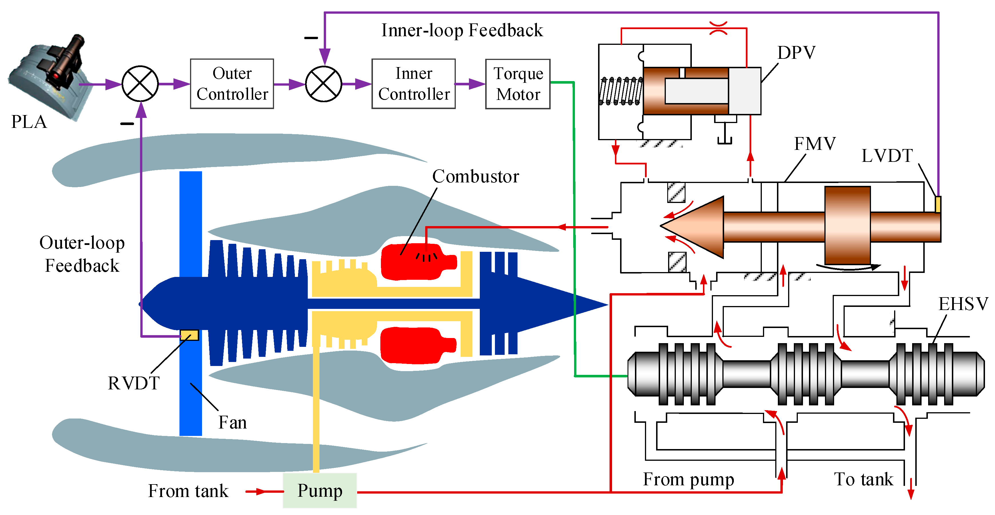
2. Cascade Electro-Hydraulic Control System of Turbofan Engine

2.1. Turbofan Engine Control System

Cascade control is an effective way to enhance the control performance of dynamic processes [26]. A cascade control system typically consists of two main control loops: the outer loop and the inner loop. By leveraging the strengths of dual-loop architecture, these systems achieve superior disturbance rejection, enhanced control accuracy, and increased stability.

Figure 1 illustrates a typical electro-hydraulic cascade control system of a turbofan engine, which comprises two primary control loops: the outer loop for fan speed control and the inner loop for fuel-metering control.

The outer loop involves a controller that regulates the fan speed based on the desired fan-speed setpoint given by the power lever angle (PLA) and the rotary variable differential transformer (RVDT). This controller adjusts the torque motor reference input of the inner-loop electro-hydraulic servo valve (EHSV), which in turn modulates the fuel flow to control the fan speed. The inner loop focuses on the precise metering of fuel delivered to the engine. The inner controller receives feedback from the linear variable differential transformer (LVDT) mounted on the fuel-metering valve (FMV) and adjusts the measured fuel flow with the aid of a difference pressure valve (DPV).

2.2. Fault Analysis of Turbofan Engine Control System

As can be seen from Figure 1, the inner-loop actuator is the EHSV-controlled FMV, the outer-loop actuator is the DPV, and LVDT and RVDT are the feedback sensors within the inner- and outer-loop, respectively. These core components are crucial to the safe and reliable operation of the entire cascade control system.

The fuel-metering unit (FMU) includes the FMV and the EHSV, and the torque motor can be regarded as part of the EHSV. Due to the harsh operational environment, the FMU is susceptible to various faults. For instance, the valve spool can wear out over time due to continuous operation and high pressures with symptoms of increased internal leakage and degraded fuel flow control. The torque motor within the EHSV can fail due to short circuits, insulation breakdown, or external damage, which results in inaccurate fuel metering or even loss of control signals.

The function of the PDV is to ensure that the pressure differential before and after the fuel-metering valve is maintained at a certain constant value so that the fuel flow rate can be controlled simply by controlling the displacement of the metering valve. Although differential valve spring fatigue or seal leakage is a multiplicative fault to the dynamics of the valve itself, the effects of common DPV faults and disturbances can be viewed as a gain fault with respect to the engine fuel output.

LVDT and RVDT are utilized to monitor the FMV openings and the fan speed; when they operate for extended periods under high temperatures and strong vibration conditions, they may experience coil breakage, changes in resistance, or even alterations in structural parameters, which can subsequently affect the related performance parameters. For example, bias and drift of sensors caused by aging, temperature changes, or calibration errors lead to persistent offset in sensor readings, leading to incorrect control responses.

It is important to note that the considered faults in this study can be uniformly modeled as an “output gain fault”, as all faults are reflected in their outputs. Therefore, the considered faults do not refer to some specific faults but represent a class of output-affecting faults that include several common fault modes.

3. Fault Diagnosis Scheme

In the cascade electro-hydraulic control system, the residual generators for fault detection in its two loops can be designed independently and specifically, tailored to the unique requirements of each control loop.

3.1. Optimal Fault Detection Filter Design for the Outer Loop System

Consider the following dynamic control system that incorporates additive disturbances and faults:

$$\left\{\begin{array}{l}{\dot{x}}_1(t)=A_1{x}_1(t)+B_1{u}_1(t)+E_{d1}{d}_1(t)+E_{f1}{f}_1(t)\\ y_1(t)=C_1{x}_1(t)+D_1{u}_1(t)+F_{d1}{d}_1(t)+F_{f1}{f}_1(t)\end{array}\right.$$

(1)

where x₁ is the state vector of outer-loop control system; y₁ signifies outer-loop output vector; A₁, B₁, C₁, and D₁ are system matrices; u₁ is the control input; d₁(t) represents the unknown disturbance input vector of the system; f₁(t) denotes the fault vector of the system; and E_d1, E_f1, F_d1, and F_f1 are the corresponding disturbance and fault matrices with appropriate dimensions.

To generate fault residuals of the outer-loop control system, the following state observer is designed:

$$\left\{\begin{array}{l}{\dot{\widehat{x}}}_1(t)=A_1{\widehat{x}}_1(t)+B_1{u}_1(t)+L_{obs}\left[y_1(t)-{\widehat{y}}_1(t)\right]\\ {\widehat{y}}_1(t)=C_1\widehat{x}(t)+D_1{u}_1(t)\end{array}\right.$$

(2)

where ${\dot{\widehat{x}}}_1$ and ${\widehat{y}}_1$ are the estimated x₁ and y₁, respectively. L_obs is the observer gain matrix that stabilizes the eigenvalues of the matrix (A₁ − L_obsC₁) stable, ensuring that the designed observer can achieve an unbiased estimate of the system state.

Define the observation residuals e_obs1 as follows:

$$e_{obs1}(t)=x_1(t)-{\widehat{x}}_1(t)$$

(3)

The dynamic characteristics of the residual generator can be described as follows:

$$\left\{\begin{array}{l}\dot{\xi }(t)={\tilde{A}}_1\xi (t)+{\tilde{E}}_{d1}{\tilde{d}}_1(t)+{\tilde{E}}_{f1}{f}_1(t)\\ r_1(t)=W\left[{\tilde{C}}_1\xi (t)+{\tilde{F}}_{d1}{\tilde{d}}_1(t)+{\tilde{F}}_{f1}{f}_1(t)\right]\end{array}\right.$$

(4)

where W is a pre-filter to be designed, r₁ is the generated system residual;

$$\begin{gathered} \xi (t)=\left[\begin{array}{c}{x}_1(t)\\ e_{obs1}(t)\end{array}\right],{\tilde{d}}_1(t)=\left[\begin{array}{c}{u}_1(t)\\ d_1(t)\end{array}\right],{\tilde{A}}_1=\left[\begin{array}{cc}{A}_1& 0\\ 0& A_1-L_{obs}{C}_1\end{array}\right], \\ {\tilde{E}}_{d1}=\left[\begin{array}{cc}{B}_1& E_{d1}\\ 0& E_{d1}-L_{obs}{F}_{d1}\end{array}\right],{\tilde{E}}_{f1}=\left[\begin{array}{c}{E}_{f1}\\ E_{f1}-L_{obs}{F}_{f1}\end{array}\right],{\tilde{C}}_1=\left[\begin{array}{cc}0& C_1\end{array}\right], \\ {\tilde{F}}_{d1}=\left[\begin{array}{cc}0& F_{d1}\end{array}\right],{\tilde{F}}_{f1}=F_{f1}. \end{gathered}$$

According to Equation (1), the transfer functions from system disturbances ${\tilde{d}}_1$ and system faults f₁ to $r_1$, respectively, are as follows:

$$G_{r_1{\tilde{d}}_1}(s)=W\left[{\tilde{F}}_{d1}+{\tilde{C}}_1\left(sI-{\tilde{A}}_1+L_{obs}{\tilde{C}}_1\right)\left({\tilde{E}}_{d1}-L_{obs}{F}_{d1}\right)\right]$$

(5)

$$G_{r_1{f}_1}(s)=W\left[{\tilde{F}}_{f1}+{\tilde{C}}_1\left(sI-{\tilde{A}}_1+L_{obs}{\tilde{C}}_1\right)\left(E_{f1}-L_{obs}{F}_{f1}\right)\right]$$

(6)

To achieve the optimal balance between the robustness of system disturbances and the sensitivity to system faults, we can solve the following optimal design problem using the theorem presented in [27] to obtain the optimal solution:

$$\underset{L_{obs},W}{\max }J(L_{obs},W)={\displaystyle \frac{{\sigma }_i\left(G_{r_1{f}_1}(\mathrm{j}\omega )\right)}{{‖G_{r_1{\tilde{d}}_1}(\mathrm{j}\omega )‖}_{\infty }}},\omega \in \left[0,\left.\infty \right)\right.$$

(7)

where ${\sigma }_i(\ast )$ is the i-th non-zero singular value, j is imaginary unit, and ω is the angular frequency.

The matrices L_obs and W that satisfy the solution of the above optimization problem could make the observer robust to disturbances while being as sensitive to faults as possible.

To detect faults, the root mean square (RMS) of the residual signal can be utilized to evaluate the energy of the residual signal:

$${‖r_1(t)‖}_{\mathrm{RMS}}=\sqrt{{\displaystyle \frac{1}{T}}{\displaystyle {\int }_t^{t+T}{r}_1^{\mathrm{T}}(\tau )r_1(\tau )\mathrm{d}\tau }}$$

(8)

where ${‖·‖}_{\mathrm{RMS}}$ represents the average energy of the residual signal within the specified time interval (t, t + T), and it can be determined based on the maximum energy value observed in the system’s historical data under fault-free conditions.

$$J_{th1,RMS}=\underset{\text{fault-free}}{\sup }{‖r_1(t)‖}_{\mathrm{RMS}}$$

(9)

By monitoring the RMS value of the residual signal and comparing it against a predetermined threshold J_th1,RMS, the fault detection logic of the outer-loop control system is given by the following:

$$\left\{\begin{array}{l}{‖r_1(t)‖}_{\mathrm{RMS}}>J_{th1,RMS}\Rightarrow \mathrm{fault}\\ {‖r_1(t)‖}_{\mathrm{RMS}}\le J_{th1,RMS}\Rightarrow \text{fault-free}\end{array}\right.$$

(10)

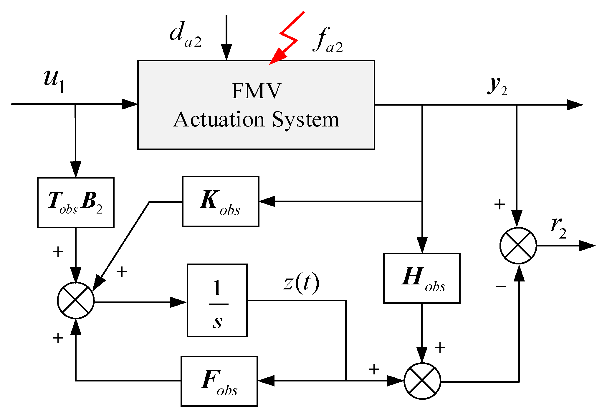
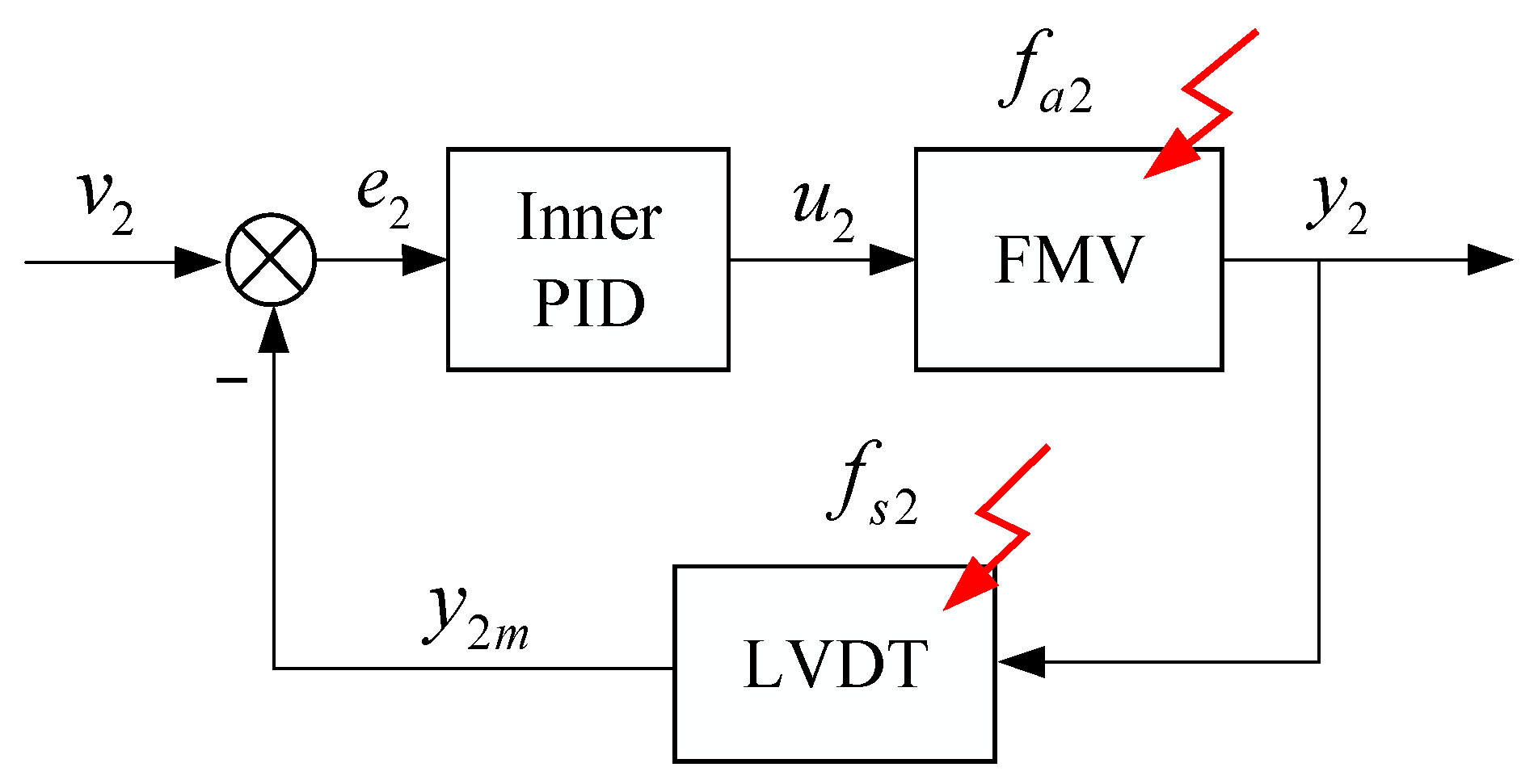
3.2. Robust Unknown Disturbance Decoupled Residual Generator for the Inner-Loop System

The inner-loop dynamic system can be described as follows:

$$\left\{\begin{array}{l}{\dot{x}}_2(t)=A_2{x}_2(t)+B_2{u}_2(t)+E_{d2}{d}_{a2}(t)\\ y_2=C_2{x}_2(t)+D_2{u}_2(t)\end{array}\right.$$

where x₂ is state vector of the inner-loop control system; y₂ is inner-loop output; A₂, B₂, C₂, and D₂ are system matrices; u₂ is control input; d_a2(t) represents the unknown external disturbance; and E_d1 is disturbance distribution matrix.

For the inner loop fuel control system dominated by multiplicative faults, an unknown disturbance decoupling observer is established as follows:

$$\left\{\begin{array}{l}\dot{z}(t)=F_{obs}z(t)+T_{obs}{B}_2{u}_2+K_{obs}{y}_2(t)\\ {\widehat{x}}_2(t)=z(t)+H_{obs}{y}_2(t)\end{array}\right.$$

(11)

where $z(t)$ is the state vector of the unknown disturbance decoupling observer; ${\widehat{x}}_2(t)$ is the estimated state vector of the inner loop; and F_obs, T_obs, K_obs, and H_obs are the observer matrices that need to be designed to achieve decoupling of additive perturbation and state estimation.

Figure 2 shows the structure of the unknown disturbance decoupling observer.

The estimated state error e_obs2 is as follows:

$$e_{obs2}(t)=x_2(t)-{\widehat{x}}_2(t)$$

(12)

The error control equation can be described as follows:

$$\begin{array}{ll}{\dot{e}}_{obs2}(t)\hfill & =(A_2-H_{obs}{C}_2{A}_2-K_{obs1}{C}_2)e_2(t)-[F_{obs}-(A_2-H_{obs}{C}_2{A}_2-K_{obs1}{C}_2)]z(t)\hfill \\ & -[K_{obs2}-(A_2-H_{obs}{C}_2{A}_2-K_{obs1}{C}_2)H_{obs}]y_2(t)\hfill \\ & -[T_{obs}-(I-H_{obs}{C}_2)]B_2{x}_{sv}(t)-(H_{obs}{C}_2-I)E_{d2}{d}_{a2}(t)\hfill \end{array}$$

(13)

where K_obs = K_obs1 + K_obs2.

When system input and output are decoupled, the state estimation error of the system can be simplified to the following:

$${\dot{e}}_{obs2}(t)=F_{obs}{e}_{obs2}(t)=\left(A_2-H_{obs}{C}_2{A}_2-K_{obs1}{C}_2\right)e_{obs2}(t)$$

(14)

If all eigenvalues of the matrix $F_{obs}$ are stable, it can be ensured that the estimation error gradually approaches zero and the estimated system states approach the true values.

According to the output of the observer and the actual output of the system, the residuals of the system can be obtained as follows:

$$r_2(t)=y_2(t)-C_2{\widehat{x}}_2(t)=(I-C_2{H}_{obs})y_2(t)-C_{2}z(t)$$

(15)

where I is an identity matrix with appropriate dimensions.

Similarly, the RMS index is utilized to evaluate the change in the residual signal, i.e.,

$${‖r_2(t)‖}_{\mathrm{RMS}}=\sqrt{{\displaystyle \frac{1}{T}}{\displaystyle {\int }_t^{t+T}{r}_2^{\mathrm{T}}(\tau )r_2(\tau )\mathrm{d}\tau }}$$

(16)

The maximum energy value of historical data recorded under fault-free conditions is used as the threshold of the residual signal:

$$J_{th2,RMS}=\underset{\text{fault-free}}{\sup }{‖r_2(t)‖}_{\mathrm{RMS}}$$

(17)

If the RMS value exceeds this threshold, a fault condition is declared. Therefore, the fault detection logic of the outer loop is as follows:

$$\left\{\begin{array}{l}{‖r_2(t)‖}_{\mathrm{RMS}}>J_{th2,RMS}\Rightarrow \mathrm{fault}\\ {‖r_2(t)‖}_{\mathrm{RMS}}\le J_{th2,RMS}\Rightarrow \text{fault-free}\end{array}\right.$$

(18)

3.3. Steady-State Propagation Characteristics of Faults in Cascade Control Systems

To analyze the propagation characteristics of actuator and sensor faults in the cascade control system, it is first necessary to derive the fault propagation characteristics of the single-loop control system shown in Figure 3.

To simplify the derivation process, multiplicative faults can be equivalently converted into additive faults [28], and the system dynamics of the inner loop can be described as follows:

$$\left\{\begin{array}{l}{\dot{x}}_2=A_2{x}_2+B_2{u}_2+E_{f2}{f}_{a2}\\ y_{2m}=C_2{x}_2+F_{f2}{f}_{s2}\end{array}\right.$$

(19)

where ${\tilde{E}}_{f2}$ is the actuator fault matrix, ${\tilde{f}}_{a2}$ is the actuator fault vector, ${\tilde{F}}_{f2}$ is the sensor fault matrix, and ${\tilde{f}}_{s2}$ is sensor fault vector.

The system matrices of the inner-loop electro-hydraulic FMV are as follows:

$$A_2=\left[\begin{array}{ccc}0& 1& 0\\ -{\displaystyle \frac{K_L}{m_t}}& -{\displaystyle \frac{B_p}{m_t}}& -{\displaystyle \frac{A_p}{m_t}}\\ 0& -{\displaystyle \frac{4{\beta }_e{A}_p}{V_t}}& -{\displaystyle \frac{4(K_{c2}+C_{ip}){\beta }_e}{V_t}}\end{array}\right],B_2=\left[\begin{array}{c}0\\ 0\\ {\displaystyle \frac{4{\beta }_e{K}_{q2}}{V_t}}\end{array}\right],C_2=\left[\begin{array}{ccc}{K}_{s2}& 0& 0\\ 0& 0& 0\\ 0& 0& 0\end{array}\right]$$

where, K_L is load stiffness of FMV, mt is mass of the FMV, A_p is the area of the FMV control chamber, B_p is damping coefficient of FMV, C_ip is the internal leakage coefficient, β_e is elastic modulus of the fuel, K_c2 is the pressure gain coefficient of EHSV, K_q2 flow gain coefficient of EHSV, V_t is volume of the FMV control chamber, and K_s2 is the LVDT gain.

The closed-loop transfer matrix from system input v₂ to output y_2m is as follows:

$${\dot{x}}_2=(A_2-B_2{C}_2{K}_2)x_2+B_2{K}_2{v}_2-B_2{\tilde{F}}_{f2}{\tilde{f}}_{s2}{K}_2+{\tilde{E}}_{f2}{\tilde{f}}_{a2}$$

(20)

where K₂ is inner-loop controller.

Then, the transfer function from system input v₂ to output y₂ is as follows:

$$G_{v_2,y_2}(s)=C_2{\left[sI-(A_2-B_2{C}_2{K}_2)\right]}^{-1}{B}_2{K}_2={\displaystyle \frac{-K_{s2}{K}_2\left[V_t{m}_t{s}^2+\left(4{\beta }_e{K}_{c2}{m}_t+V_t{B}_p\right)s+4{\beta }_e{A}_p^2\right]}{V_t{m}_t{s}^3+\left(4{\beta }_e{K}_{c2}{m}_t+V_t{B}_p\right)s^2+4{\beta }_e{A}_p^{2}s+4{\beta }_e{A}_p{K}_{s2}{K}_2{K}_{q2}}}$$

(21)

From Equation (21), it can be observed that feedback sensor gain K_s2 and controller K₂ have direct impacts on the system output under the closed-loop control situation.

Similarly, the transfer functions of the actuator faults to the specific signals in the loop $G_{u_2,f_{a2}}$, $G_{y_2,f_{a2}}$, $G_{y_{2m},f_{a2}}$, $G_{u_2,f_{s2}}$, $G_{y_2,f_{s2}}$, and $G_{y_{2m},f_{s2}}$ can be obtained.

The steady-state outputs of the derived system transfer functions can be calculated, respectively, using the final value theorem, and results are as follows:

$$\underset{s\to 0}{\lim }\left[s{F}_{a2}(s)G_{u_2,f_{a2}}(s)\right]=0,\underset{s\to 0}{\lim }\left[s{F}_{a2}(s)G_{y_2,f_{a2}}\right]=0,\underset{s\to 0}{\lim }\left[s{F}_{a2}(s)G_{y_{2m},f_{a2}}\right]=0,$$

$$\underset{s\to 0}{\lim }\left[s{F}_{s2}(s)G_{u_2,f_{s2}}\right]=0,\underset{s\to 0}{\lim }\left[s{F}_{s2}(s)G_{y_2,f_{s2}}\right]=-{\displaystyle \frac{F_{f2}}{K_{s2}}},\underset{s\to 0}{\lim }\left[s{F}_{s2}(s)G_{y_{2m},f_{s2}}\right]=0,$$

It can be seen from the above calculation results that, for a single-loop closed-loop control system, feedback sensor faults will affect the steady-state control accuracy of the closed-loop control system, and the control error is directly related to the faulty sensor gain. In contrast, actuator faults usually do not affect the actual steady-state output of the system. Furthermore, neither actuator faults nor sensor faults affect the steady-state values of the measured output y_2m and the control input u₂ within the loop.

The fault propagation characteristics of a single closed-loop system are summarized in

Table 1. Steady-state propagation characteristics of inner-loop typical faults of a turbofan engine.

Fault/Disturbance	Control Input	Actual Output	Measured Output
FMV disturbance	N	N	N
FMV Leakage	N	N	N
LVDT gain bias	N	Y	N

Note: symbol ‘N’ indicates that when a fault occurs, the steady-state residual signal quickly approaches zero after a short adjustment period, while the symbol ‘Y’ signifies that the steady-state residual signal converges to a non-zero value.

.

As evident from Table 1, additive disturbances in the system do not affect the final steady-state control characteristics of the system. This underscores the robustness of the closed-loop control system, which is capable of mitigating the effects of process disturbances in the system, except in cases of feedback sensor faults or other disturbances.

Nonetheless, when considering the presence of the external control loop as depicted in Figure 4, the conclusion changes. In this scenario, the steady-state error of the inner loop system’s actual output is further corrected by the outer controller, thereby altering the steady-state outputs of multiple signals within the loop.

The analytical derivation method can be employed to obtain the transfer functions between different signals in the cascade control system. Additionally, the steady-state propagation characteristics of faults within the cascade fuel control system are presented in

Table 2. Steady-state propagation characteristics of faults in a turbofan cascade control system.

Faults/Disturbance	u1	y1	y1m	v2	u2	y2	y2m
FMV leakage	N	N	N	Y	Y	N	N
LVDT gain bias	N	N	N	Y	N	N	Y
DPV fault	N	N	N	Y	N	Y	Y
RVDT gain bias	Y	Y	N	Y	N	Y	Y

Note: Symbols ‘N’ and ‘Y’ have the same meaning as in Table 1.

.

According to the previous analysis, when the feedback sensor in the inner loop experiences a gain failure, it results in a deviation in the control input command of the fuel servo mechanism. This, in turn, leads to changes in the actual outputs of the fuel-metering valve, fuel flow, and engine rotor speed. However, the outer-loop controller corrects the deviations by adjusting the command of the inner-loop actuator, effectively eliminating the engine speed deviation and maintaining the measured rotation speed at the reference value.

3.4. Fault Isolation Scheme Based on Steady-State Fault Propagation Characteristics

To isolate the fault, define the minimum dimension residual vector r_sys(t) of the cascade control system:

$$\begin{array}{ll}{r}_{sys}(t)\hfill & =\left[\begin{array}{ccccc}\left|\Delta u_1(t)\right|,& \left|\Delta v_2(t)\right|,& \left|\Delta u_2(t)\right|,& \left|\Delta y_2(t)\right|,& \left|\Delta y_{2m}(t)\right|\end{array}\right]\\ & =\left[\begin{array}{ccccc}\left|u_1(t)-u_{10}\right|,& \left|v_2(t)-v_{20}\right|,& \left|u_2(t)-u_{20}\right|,& \left|y_2(t)-y_{20}\right|,& \left|y_{2m}(t)-y_{2m0}\right|\end{array}\right]\hfill \end{array}$$

(22)

where u₁₀ represents the nominal value of fuel flow, and v₂₀ is the nominal output of the outer-loop controller, which also serves as the nominal command value for the inner loop. Additionally, u₂₀ denotes the nominal output of the inner-loop controller, y₂₀ represents the nominal output of the inner-loop servo actuator, and y_2m0 is the nominal measurement output of the inner-loop feedback sensor.

These nominal status values can all be derived from the system’s fault-free historical operating data, which have been collected under different working conditions. Based on real-time monitoring data or offline data, the signal residual vector of the fuel-speed cascade control system can be calculated.

Assuming that the system can experience four distinct faults: inner-loop actuator failure, inner-loop feedback sensor failure, outer-loop actuator failure and, outer-loop feedback sensor failure, with no more than one fault occurring simultaneously, then the fault influence distribution matrix M is obtained by analyzing the steady-state propagation characteristics of actuator and sensor faults within the cascade control system:

$$M={\left[\begin{array}{ccccc}0& 1& 1& 0& 0\\ 0& 1& 0& 0& 1\\ 0& 1& 0& 1& 1\\ 1& 1& 0& 1& 1\end{array}\right]}_{4\times 5}$$

To prevent the occurrence of ill-conditioned matrices, which can arise due to significant differences in the magnitudes of various residuals, and to enhance the accuracy of fault isolation, it is necessary to normalize each residual vector using the following formula:

$${\overline{r}}_{sys}^q(t)={\displaystyle \frac{r_{sys}^q(t)-r_{sys}^q(t){|}_{\min }}{r_{sys}^q(t){|}_{\max }-r_{sys}^q(t){|}_{\min }}}\left(q=1,2,3,4,5\right)$$

where q represents the q-th column in the residual vector r_sys(t), and the maximum and minimum values of the residual vector can be obtained from the fault-free historical operation data of the system in the past period.

Assume that the p-th row vector of fault influence distribution matrix M^p$(p=1,2,3,4)$ represents four typical fault modes: f_a2, f_s2, f_a1, and f_s1, then calculate the vector angles between the normalized residual vector ${\overline{r}}_{sys}$ and each row vector of fault influence distribution matrix M. The value of p that minimizes the vector angle value is the result of fault isolation, i.e.:

$$\arg \underset{p}{\max }\left\{\cos 〈M^p\cdot {\overline{r}}_{sys}^q〉\right\},(p=1,2,3,4)$$

(23)

4. Experiments

To validate the effectiveness of the proposed fault isolation scheme, experiments were conducted on an electro-hydraulic servo system test bench. This test bench is capable of simulating the cascade control system of a turbofan engine. Figure 5 shows the composition and principle of experimental setup. It includes pump source, electro-hydraulic servo actuator, virtual engine simulation system, and real-time measurement and control system. The considered faults can be simulated by changing the signal gains in the real-time virtual engine simulation system. Figure 6 presents on-site testing image, where the cylinder can be regarded as the FMV.

The midpoint of the FMV’s maximum stroke was selected as the operating point, corresponding to a fuel flow rate of 1.0 Kg/s. At this fuel flow rate, the engine speed is 10,000 r/min. The engine model can be simplified to a first-order system with a adjustment time of approximately 4 s.

$$G_{Eng}(s)={\displaystyle \frac{10000}{0.7s+1}}$$

It is important to note that the accuracy of the proposed fault diagnosis method does not depend on the accuracy of the engine model, because it is based on steady-state characteristics, so it is reasonable to choose a first-order inertia link to simulate the fan speed of a turbofan engine.

In the experiment, the system pressure was set to 21 MPa, and the sampling time was 0.001 s. Both of the two-loop controllers employed are simple proportional controllers. The servo valve-controlled cylinder simulates the FMV with a total stroke of 30 mm. Within the host computer software, deviation faults were artificially injected into the outputs of the actuators and sensors, respectively. Subsequently, all output signals in the cascade control system, namely u₁, y₁, y_1m, v₂, u₂, y₂, and y_2m, were collected.

Figure 7 illustrates the differential effects of four typical faults on the inner-loop signals within the cascade control system. As seen in Figure 7a,b, when deviation faults are introduced at 1.0 s, the reference input v₂ and control input u₂ gradually stabilize after approximately four seconds of adjustment. However, a noticeable steady-state error persists, especially in the case of RVDT gain deviation faults.

Comparing Figure 7c,d, a significant deviation is observed between the actual and measured outputs of the metering valve when the LVDT is faulty, which is unacceptable for practical engine control applications. Conversely, when a deviation fault occurs in the FMV, the actual and measured output signals of the metering valve gradually converge to a stable value after three seconds of dynamic adjustment, with minimal steady-state error compared to the fault-free system. However, DPV and RVDT faults significantly affect the actual and measured outputs of the metering valve, resulting in substantial steady-state errors.

As shown in Table 2, when a deviation fault occurs in the FMV, the steady-state residuals of the signals v₂, u₂, y₂, and y_2m ultimately approach zero after a brief adjustment period, as demonstrated in Figure 7. However, an interesting phenomenon arises during the dynamic adjustment: the initial change in the system’s actual and measured output signal residuals aligns with the fault direction, while the control input residual changes in the opposite direction. This is due to the closed-loop controller’s corrective action; upon detecting a deviation in the measured output, the control input adjusts in the opposite direction to mitigate the fault’s impact. Conversely, when a deviation fault occurs in the LVDT sensor, the initial change in the measured output aligns with the fault, but the control input and actual output residuals change in the opposite direction, indicating a corrective response by the system.

Figure 8 shows that for the outer-loop control system, among the four typical fault modes, the RVDT fault has the most significant impact on the outer-loop signals. The effects of the other three faults are mitigated by the corrective actions of the closed-loop controller. This finding aligns with the theoretical results discussed earlier and underpins the subsequent fault isolation scheme based on steady-state propagation characteristics. It is important to note that due to the first-order engine model and the difference between the two cascade controllers, some signals exhibit significant noise while others appear filtered. For example, the signal noise from the inner-loop feedback sensor is greatly reduced after passing through the engine model.

According to the experimental data, the steady-state residual values of each signal under four different fault conditions and fault-free conditions were calculated. The results are summarized in

Table 3. Steady-state residuals under different fault conditions.

Fault Location	u1	y1	y1m	v2	u2	y2	y2m
FMV	0.33458	1.45745	1.45745	−1.45745	−0.00049	0.00418	0.00418
LVDT	−0.16846	−7.08437	−7.08437	7.08437	0.00232	−0.00211	0.49730
DPV	−0.02578	−1.73491	−1.73491	1.73492	0.00065	−0.83297	−0.83297
RVDT	−37.486500	−941.745	−36.4096	36.40957	0.01218	−0.46858	−0.46858

.

Based on the experimental data, we can obtain the normalized residual matrix as follows:

$${\overline{r}}_{sys}=\left[\begin{array}{ccccc}0.2230& 1.0000& 0.9975& 0.1254& 0.1254\\ 0.0075& 0.3259& 0.3192& 0.0042& 1.0000\\ 0.0007& 0.0477& 0.0532& 1.0000& 1.0000\\ 1.0000& 1.0000& 1.0000& 0.5625& 0.5625\end{array}\right]$$

The fault isolation results can be determined by computing the vector angles between each fault’s normalized residual vector and each row vector of the fault influence distribution matrix M. The results are shown in

Table 4. The fault isolation results of the proposed method in this study.

Vector Angle	M1	M2	M3	M4	Isolation Results
$\mathrm{ac}\cos 〈M^1\cdot {\overline{r}}_{sys}^1〉$	11.40°	31.72°	38.72°	39.91°	p = 1
$\mathrm{ac}\cos 〈M^2\cdot {\overline{r}}_{sys}^2〉$	65.48°	31.46°	45.68°	52.52°	p = 2
$\mathrm{ac}\cos 〈M^3\cdot {\overline{r}}_{sys}^3〉$	87.11°	58.45°	33.39°	43.67°	p = 3
$\mathrm{ac}\cos 〈M^4\cdot {\overline{r}}_{sys}^4〉$	42.10°	54.57°	49.93°	34.94°	p = 4

.

Table 4 shows that the minimum angles between the four residual vectors and each row vector of the fault influence distribution matrix M are 11.40°, 31.46°, 33.39°, and 34.94°, corresponding to the FMV, LVDT, DPV, and RVDT faults, respectively. In practical applications, targeted maintenance can be performed based on these isolation results, particularly using the minimum and sub-minimum angle values, to enhance the reliability of diagnostic outcomes and improve maintenance efficiency.

5. Discussion and Conclusions

This study deals with the fault diagnosis of the cascade electro-hydraulic control system of a turbofan engine. We propose a novel fault isolation scheme based on the steady-state propagation characteristics within the control loops. Conclusions are drawn as follows:

In a single closed-loop control system, the feedback controller can result in the steady-state effects of actuator disturbances and faults being transferred, attenuated, or even completely mitigated within the control loops, except for the feedback sensor fault. In a cascade control system, the inner-loop sensor fault effects can be compensated via the outer-loop sensor and controller. Similarly, the impact of the outer-loop actuator faults can be mitigated by adjusting the reference command of the inner loop. Only the health status of the outer-loop sensor directly influences the final controlled variable of the entire system. This influence cannot be mitigated by the closed-loop correction effect inherent to the cascade control system. Considering the steady-state propagation effects of these faults, the proposed method for constructing a minimum dimensional residual vector and a fault influence distribution matrix to characterize the health state of the cascade control system simplifies fault isolation to a straightforward mathematical problem of calculating vector angles. The experimental results demonstrate that this method effectively locates faults within the cascade control system, which provides a solid foundation for subsequent repair and maintenance activities.

The novel fault isolation method proposed in this paper is not only applicable to single closed-loop control systems, but also to cascade or even multi-loop feedback control systems. The essence of this method lies in acquiring the steady-state propagation characteristics of different faults within the cascade control system, whether through analytical methods or simulated experiments, and thereby determining the fault influence distribution matrix of the system. As more fault modes are considered, an increased number of characteristic signals within the loop are required, leading to a higher-dimensional fault influence distribution matrix. Consequently, this matrix is not unique, but there exists a matrix with minimal dimension. The smaller the matrix dimension, the less computing resources are required for calculation, which is essential for both online real-time and offline fault diagnosis. Additionally, by leveraging the linear combination of the row vectors of the fault influence distribution matrix, the behavior of signals within the loop under simultaneous multiple faults can be discerned. Therefore, this method shows considerable promise in multi-fault diagnosis. With the method we proposed, it would be possible to detect a control error produced by the control. Therefore, the proposed method can be used for fault-tolerant control. Our future work will focus on multi-fault isolation designs, performance monitoring, and demand-driven optimization of sensor redundancy layouts of cascade control systems.

References

1. Ba, K.X.; Chen, C.H.; Ma, G.L.; Song, Y.H.; Wang, Y.; Yu, B.; Kong, X.D. A compensation strategy of end-effector pose precision based on the virtual constraints for serial robots with RDOFs. Fundam. Res. 2024. [Google Scholar] [CrossRef]
2. Zhang, Y.; Wang, S.P.; Shi, J.; Wang, X. Evaluation of thermal effects on temperature-sensitive operating force of flow servo valve for fuel metering unit. Chin. J. Aeronaut. 2020, 33, 1812–1823. [Google Scholar] [CrossRef]
3. Kim, D.; Park, H.J.; Kim, S.S.; Kim, D.H.; Kim, S.B.; Lee, J.; Choi, J.Y. Position control of dual redundant asymmetric tandem electro-hydrostatic actuator for aircraft based on backstepping technique. J. Aerosp. Syst. Eng. 2021, 15, 1–10. [Google Scholar]
4. Zhou, T.; Zhang, L.; Han, T.; Droguett, E.L.; Mosleh, A.; Chan, F.T.S. An uncertainty-informed framework for trustworthy fault diagnosis in safety-critical applications. Reliab. Eng. Syst. Saf. 2023, 229, 108865. [Google Scholar] [CrossRef]
5. Azarbani, A.; Fakharian, A.; Menhaj, M.B. On the design of an unknown input observer to fault detection, isolation, and estimation for uncertain multi-delay nonlinear systems. J. Process Control. 2023, 128, 103018. [Google Scholar] [CrossRef]
6. Jyotish, N.K.; Singh, L.K.; Kumar, C.; Singh, P. Reliability and performance measurement of safety-critical systems based on petri nets: A case study of nuclear power plant. IEEE Trans. Reliab. 2023, 72, 1523–1539. [Google Scholar] [CrossRef]
7. Pourtakdoust, S.H.; Mehrjardi, M.F.; Hajkarim, M.H.; Gourabi, F.N. Advanced fault detection and diagnosis in spacecraft attitude control systems: Current state and challenges. Proc. Inst. Mech. Eng. Part G J. Aerosp. Eng. 2023, 237, 2679–2699. [Google Scholar] [CrossRef]
8. Attouri, K.; Dhibi, K.; Mansouri, M.; Hajji, M.; Bouzrara, K.; Nounou, H. Enhanced fault diagnosis of wind energy conversion systems using ensemble learning based on sine cosine algorithm. J. Eng. Appl. Sci. 2023, 70, 1–16. [Google Scholar] [CrossRef]
9. Wang, Y.L.; Pan, Z.F.; Yuan, X.F.; Yang, C.H.; Gui, W.H. A novel deep learning-based fault diagnosis approach for chemical process with extended deep belief network. ISA Trans. 2020, 96, 457–467. [Google Scholar] [CrossRef]
10. Hasan, A.; Tahavori, M.; Midtiby, H.S. Model-based fault diagnosis algorithms for robotic systems. IEEE Access 2023, 11, 2250–2258. [Google Scholar] [CrossRef]
11. Abbaspour, A.; Aboutalebi, P.; Yen, K.K.; Sargolzaei, A. Neural adaptive observer-based sensor and actuator fault detection in nonlinear systems: Application in UAV. ISA Trans. 2017, 67, 317–329. [Google Scholar] [CrossRef]
12. Poon, J.; Jain, P.; Konstantakopoulos, I.C.; Spanos, C.; Panda, S.K.; Sanders, S.R. Model-based fault detection and identification for switching power converters. IEEE Trans. Power Electron. 2016, 32, 1419–1430. [Google Scholar] [CrossRef]
13. Jihani, N.; Kabbaj, M.N.; Benbrahim, M. Sensor fault detection and isolation for smart irrigation wireless sensor network based on parity space. Int. J. Electr. Comput. Eng. 2023, 13, 1463. [Google Scholar] [CrossRef]
14. Du, Y.; Budman, H.; Duever, T.A. Integration of fault diagnosis and control based on a trade-off between fault detectability and closed loop performance. J. Process Control. 2016, 38, 42–53. [Google Scholar] [CrossRef]
15. Safaeipour, H.; Forouzanfar, M.; Casavola, A. A survey and classification of incipient fault diagnosis approaches. J. Process Control. 2021, 97, 1–16. [Google Scholar] [CrossRef]
16. Sun, B.W.; Wang, J.Q.; He, Z.M.; Qin, Y.R.; Wang, D.Y.; Zhou, H.Y. Fault detection for closed-loop control systems based on parity space transformation. IEEE Access 2019, 7, 75153–75165. [Google Scholar] [CrossRef]
17. Kong, X.D.; Cai, B.P.; Liu, Y.H.; Zhu, H.M.; Yang, C.; Gao, C.T.; Liu, Y.Q.; Liu, Z.K.; Ji, R.J. Fault diagnosis methodology of redundant closed-loop feedback control systems: Subsea blowout preventer system as a case study. IEEE Trans. Syst. Man Cybern. Syst. 2022, 53, 1618–1629. [Google Scholar] [CrossRef]
18. Liu, Y.; Wang, Z.D.; He, X.; Zhou, D.H. A class of observer-based fault diagnosis schemes under closed-loop control: Performance evaluation and improvement. IET Control. Theory Appl. 2017, 11, 135–141. [Google Scholar] [CrossRef]
19. Sun, B.W.; Wang, J.Q.; He, Z.M.; Zhou, H.Y.; Gu, F.S. Fault identification for a closed-loop control system based on an improved deep neural network. Sensors 2019, 19, 2131. [Google Scholar] [CrossRef]
20. Cheng, Y.; Wang, R.X.; Xu, M.Q. A combined model-based and intelligent method for small fault detection and isolation of actuators. IEEE Trans. Ind. Electron. 2015, 63, 2403–2413. [Google Scholar] [CrossRef]
21. Grehan, J.; Ignatyev, D.; Zolotas, A. Fault detection in aircraft flight control actuators using support vector machines. Machines 2023, 11, 211. [Google Scholar] [CrossRef]
22. Zhang, Z.T.; Zhang, X.F.; Yan, T.H.; Gao, S.; Yu, Z. Data-driven fault detection of AUV rudder system: A mixture model approach. Machines 2023, 11, 551. [Google Scholar] [CrossRef]
23. Jia, F.L.; Cao, F.F.; Guo, Y.Q.; He, X. Active fault diagnosis for a class of closed-loop systems via parameter estimation. J. Frankl. Inst. 2022, 359, 3979–3999. [Google Scholar] [CrossRef]
24. Niemann, H.; Poulsen, N.K. Fault Detection in Closed-Loop Systems Using a Double Residual Generator. In Proceedings of the 2022 11th IFAC Symposium on Fault Detection, Supervision and Safety for Technical Processes, Pafos, Cyprus, 8–10 June 2022. [Google Scholar]
25. Zhang, Y.; Wang, S.P.; Shi, J.; Yang, X.Y.; Zhang, J.R.; Wang, X. SAR performance-based fault diagnosis for electro-hydraulic control system: A novel FDI framework for closed-loop system. Chin. J. Aeronaut. 2022, 35, 381–392. [Google Scholar] [CrossRef]
26. Wang, Y.; Zhao, J.; Ding, H.; Zhang, H. Nonlinear cascade control of an electro-hydraulic actuator with large payload variation. Asian J. Control. 2023, 25, 101–113. [Google Scholar] [CrossRef]
27. Ding, S.X. Advanced Methods for Fault Diagnosis and Fault-Tolerant Control, 1st ed.; Springer: Berlin/Heidelberg, Germany, 2021; pp. 91–95. [Google Scholar]
28. Ding, S.X. Model-Based Fault Diagnosis Techniques: Design Schemes, Algorithms, and Tools; Springer: Berlin/Heidelberg, Germany, 2013; pp. 28–29. [Google Scholar]
Figure 1. Cascaded electro-hydraulic control system of a turbofan engine.
Machines 12 00600 g001
Figure 2. Structure of robust unknown disturbance decoupled residual generator.
Machines 12 00600 g002
Figure 3. Inner-loop actuator and feedback sensors faults.
Machines 12 00600 g003
Figure 4. Outer-loop actuator and feedback sensors faults.
Machines 12 00600 g004
Figure 5. Schematic diagram of the electro-hydraulic test bench. 1—Stop valve; 2—Hydraulic pump; 3—Relief valve; 4—Check valve; 5—Accumulator; 6—EHSV; 7—Hydraulic cylinder; 8—Displacement sensor; 9—DPV model; 10—Engine model; 11—Rotation speed sensor; 12—Outer controller; 13—Inner controller; 14—Amplifier.
Machines 12 00600 g005
Figure 6. Test bench of the electro-hydraulic control system.
Machines 12 00600 g006
Figure 7. Inner-loop propagation characteristics of different fault conditions. (a) Inner-loop reference input. (b) Inner-loop control input. (c) Inner-loop actual output. (d) Inner-loop measured output.
Machines 12 00600 g007
Figure 8. Outer-loop propagation characteristics of different fault conditions. (a) Reference input of outer-loop engine. (b) Actual output of outer-loop engine. (c) Measured output of outer-loop engine.
Machines 12 00600 g008