Abstract
The large lateral displacement of tail ropes increases the risk of their wear and fracture, posing hidden dangers to the safety of the hoisting system. However, no suitable method is available to recognize the lateral swing of tail ropes online. A target-free visual measurement method, which includes the dual-branch SiamSeg, was proposed in this study. Considering the slender characteristics of tail ropes, the receptive field of the feature extraction network was enhanced via the Receptive Field Module (RFM), thereby strengthening the discriminability and integrity of tail rope features. The consistency loss constraints were added to the segmentation loss function to maximize the time sequence information of the video and further improve the accuracy of pixel-level displacement. Compared with other methods, the proposed approach achieved better segmentation effects. Comparison results synchronously measured by sensors revealed the effectiveness of this method and its potential for practical underground applications.
1. Introduction
Mine hoisting transportation is a crucial link in the process of coal production. In the complex and harsh mine environment, the reliability of the mine hoisting system not only directly affects the production efficiency of enterprises but also closely relates to the safety of staff. With the mining of deep coal, the mine hoist is becoming increasingly large-scale and efficient, accompanied by a rise in equipment operation and maintenance costs. Numerous scholars have widely focused on improving effective system monitoring via various sensors. The friction hoisting system, which is mainly responsible for the transportation of coal, equipment, and personnel on the ground and underground, has been extensively utilized in coal mining and transportation because of its advantages of large single hoisting capacity, low derrick construction cost, and short construction period. As an important part of the friction hoisting system, the tail rope plays a balancing role while connecting lifting and lowering containers. The hoist is a piece of periodic equipment. Therefore, frequent acceleration and deceleration and disturbance excitation trigger the lateral displacement of the tail ropes during the operation of the hoisting system. If the lateral swing amplitude is large, then risks such as collision between tail ropes and the shaft wall will be induced, which will lead to the intense wear of tail ropes and seriously affect the safety operation of the system if they last for a long time. The swing amplitude of tail ropes will be enlarged as the hoisting depth increases, and the risk of colliding with the rope-splitting beam, shaft, and other underground facilities will be considerably aggravated, even causing fractures of wires and strands and further triggering major accidents. Such accidents have been reported at home and abroad. In 2004, the tail rope collided with the guide beam in the main shaft of Baodian Coal Mine, Shandong Province, China, generating sparks. For the sake of safety, the mine was immediately subjected to a production halt and overhaul to avoid further aggravating the accident. Multiple tail rope accidents also occurred once at the new shaft hoist in Junde Mine, Heilongjiang, China, during which broken ropes damaged all kinds of equipment in the shaft and even endangered the lives of people in the cage. In 2011, the tail rope in the main shaft of Beiminghe Iron Mine, Hebei Province, China, broke and fell into the shaft, and the entire mine was shut down for 96 h despite no casualties. In 2021, the tail rope broke in the main shaft of Nandong Mine in Zambia, causing substantial economic losses. Therefore, high importance should be attached to the lateral swing of the tail rope to protect the hoisting system from potential safety hazards. In addition, the lateral swing of tail ropes is one piece of vital information indicating their operating health status, from which the operating status of tail ropes can be determined. The monitoring of such information can provide an experimental basis and data support for the follow-up research on the inhibition of the tail rope swing and the safety enhancement of the hoisting system. Hence, monitoring the lateral swing of tail ropes is an indispensable link in the health monitoring of the process system, and acquiring the lateral swing data of tail ropes of shaft hoists is of considerable importance for ensuring the safe operation of the friction hoisting system.
Tail ropes operate underground for a long time, and the hoisting system is scarcely shut down. Therefore, manual observation of their swing status in real time is difficult, thus urgently needing an intelligent online swing monitoring method. At present, the existing swing measurement methods can be divided into two major types: contact and noncontact measurements [1]. Contact measurement methods have been widely applied to research in fields other than the aforementioned fields [2,3,4]. For the lateral vibration measurement of wire ropes, Kou Baofu et al. [5] fixed an Integrated Circuits Piezoelectric (ICP) deceleration sensor on the wire rope and performed wireless acquisition of the lateral vibration of the hoisting rope. However, this method has certain limitations. First, arranging common contact displacement sensors on a flexible body in operation is difficult. Second, the measurement object in this study is the tail rope, which is freely suspended during the operation of the hoisting system, and the contact measurement will lead to certain changes in the properties, such as stiffness, mass, and structure of the measurement object, thus affecting its operating status and failing to reflect its dynamic performance directly. Therefore, such contact measurement methods as displacement sensors cannot be adopted. Extensive attention has then been paid to noncontact measurement techniques for the swing monitoring of tail ropes, including laser ranging [6,7], ultrasonic measurement [8], magnetic measurement [9], and visual measurement [10]. Given the particularity of the underground environment, the tail rope is located at the bottom of the hoisting container, and the environment in the wellbore is harsh. Moreover, some laser and ultrasonic detection equipment is expensive, the installation procedures are complicated, and the operation is difficult. The measurement results are also easily affected by the environment, increasing the difficulty in addressing the measurement requirements. By contrast, if a visual measurement method is adopted, then taking the recorded target video as the monitoring information through the fixed camera, followed by a series of processing and analysis steps, is only necessary to obtain swing information. Compared with more localized contact displacement sensors, the visual method can consider each pixel point of the tail rope in the image a sensor, which not only realizes large-scale swing measurement of the tail rope but also facilitates fixed-point monitoring of lateral swing. Hence, the practicality of engineering applications can be enhanced by developing a method that completes target-free real-time monitoring of multipoint dynamic displacement only by relying on ordinary low-cost cameras.
In addition, the visual measurement method, which integrates the advantages of noncontact, easy installation and cost-effectiveness, has been rapidly developed in recent years. At present, this method has been widely used in various fields [11], such as component measurement [12,13], agricultural breeding [14], and cultural heritage protection [15]. In the engineering field, vision-based displacement measurement has become a highly promising technique. Khuc et al. implemented vision-based displacement measurement using UAVs and determined the swing displacement of a tower structure [16]. Xu et al. measured the structural displacement of a large-span highway bridge by combining a Siamese tracker and the template matching technique [17]. Lee et al. introduced an estimation method for rope displacement from lateral views [18]. Considering the vision-based measurement method, artificial markers must generally be attached to the measured object to effectively assist in the recognition and tracking of monitoring points (e.g., installing LED or the target panel as the tracking targets) [19,20,21]. Given the high color contrast of such artificial markers, segmenting these markers from the image background for follow-up tracking and measurement is easy. However, such methods with markers demonstrate poor applicability in practical engineering applications, and realizing comprehensive measurement by attaching marked points at each part of the tail rope is not feasible.
Therefore, some scholars have begun to study the target-free visual measurement technique. Bhowmick [22] proposed a method to track the time-dependent changes in the continuous edge of the tracking target to obtain the displacement response of the cantilever beam. However, this method is limited by the substantially lower texture of the background compared with that of the target edge, increasing its unsuitability for the complex environment where the tail rope is located. Xu et al. [23] identified the displacement of bridge cables through edge detection and motion estimation. Won et al. [24] measured the displacement of the cantilever beam by combining Deepmatching and Deepflow measurements. Such methods obtain the displacement by matching feature points based on the target edge or feature point detection. However, each point of the tail rope space displays the same color or gray features, complicating the selection of accurate feature reference points in the measurement of lateral swing. Yu et al. [25] optimized the EDLines detector by setting new screening strategies to effectively identify the displacement response of the ropes of cable-stayed bridges. Different from the curved bottom formed by the natural suspension of the tail rope, the rope of cable-stayed bridges is tensioned, and the slender and straight rope can be regarded as a line segment. This type of detector can specifically detect the straight line or line segment features of the ropes of cable-stayed bridges. Caetano [26] analyzed the change in pixel intensity from the video of bridge ropes using optical flow estimation and further detected the vibration of the ropes. However, this method is not only sensitive to illumination variation but also susceptible to the target shade, resulting in the inaccuracy of calculations.
Based on the above discussion, a vision-based online measurement system for the swing displacement of the tail rope, which could provide reliable displacement information and improve the health monitoring of the hoisting system, was designed in this study. The main contributions of this study are described as follows: (1) An experimental platform for the lateral swing of the tail rope was set up to provide simulation data for the visual measurement model. Next, a dual-branch network, SiamSeg, which is used for the lateral swing measurement of the tail rope, was proposed. When extracting the features of the tail rope, the receptive field of the model was enhanced using the RFM model to improve the quality of feature representation. (2) Given the small proportion of the tail rope in the video frame, two loss functions were adopted, among which the auxiliary loss function could make full use of the time sequence information in the video and enhance the accuracy of the algorithm. (3) The lateral swing characteristics of the tail rope at different monitoring points under various operating conditions were summarized. The region with the maximum swing of the tail rope was identified, which was convenient for providing effective monitoring points for visual monitoring and saving on health monitoring costs.
The remainder of this paper is organized as follows: Section 2 comprehensively introduces the measurement process for the lateral swing of the tail rope and the proposed method. Section 3 analyzes and discusses the experimental results of the proposed method. Section 4 draws the research conclusions.
2. Method
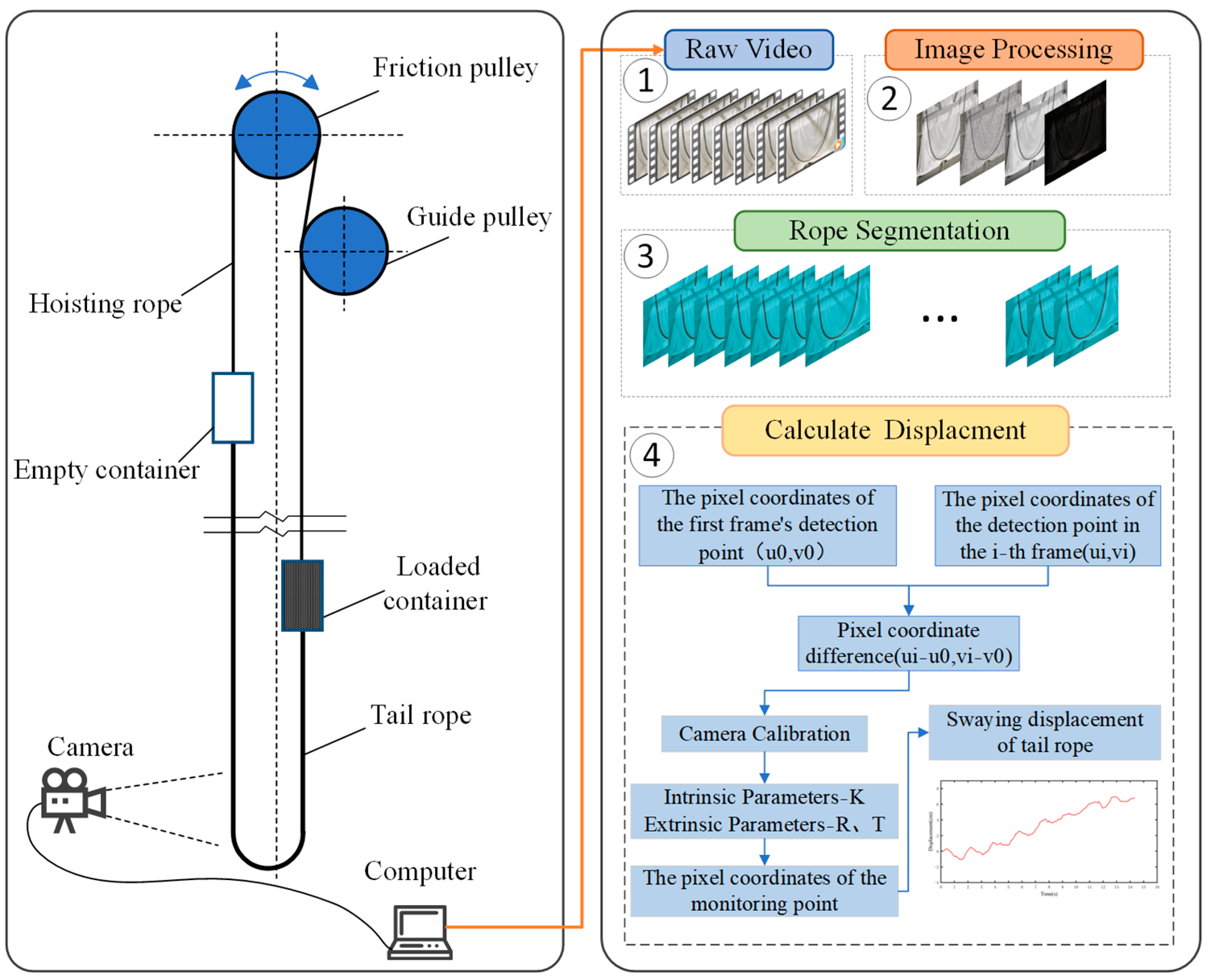
Figure 1 shows the working flowchart for measuring the lateral swing displacement of the hoist tail rope from the obtained video of the tail rope. The system comprises a tail rope, a camera, a computer, and an internal measurement algorithm. First, the real-time captured video was preprocessed. Then, the position of the tail rope in the video frame was determined, and the tail rope video captured by the camera was segmented using the trained model to obtain new video data only containing the tail rope. Finally, the lateral swing displacement of the tail rope in the real world was calculated through a coordinate transformation.

Figure 1.
Visual measurement schematic.
In order to solve the problem that there are no obvious features in the tail rope video captured by the camera, a new model was proposed to determine the position of the tail rope in the video frame and calculate its lateral swing displacement. Given an input video sequence, this study aimed to segment the tail rope and obtain the pixel-wise displacement of the tail rope. The details will be explained in the following sections.
2.1. Rope Segmentation
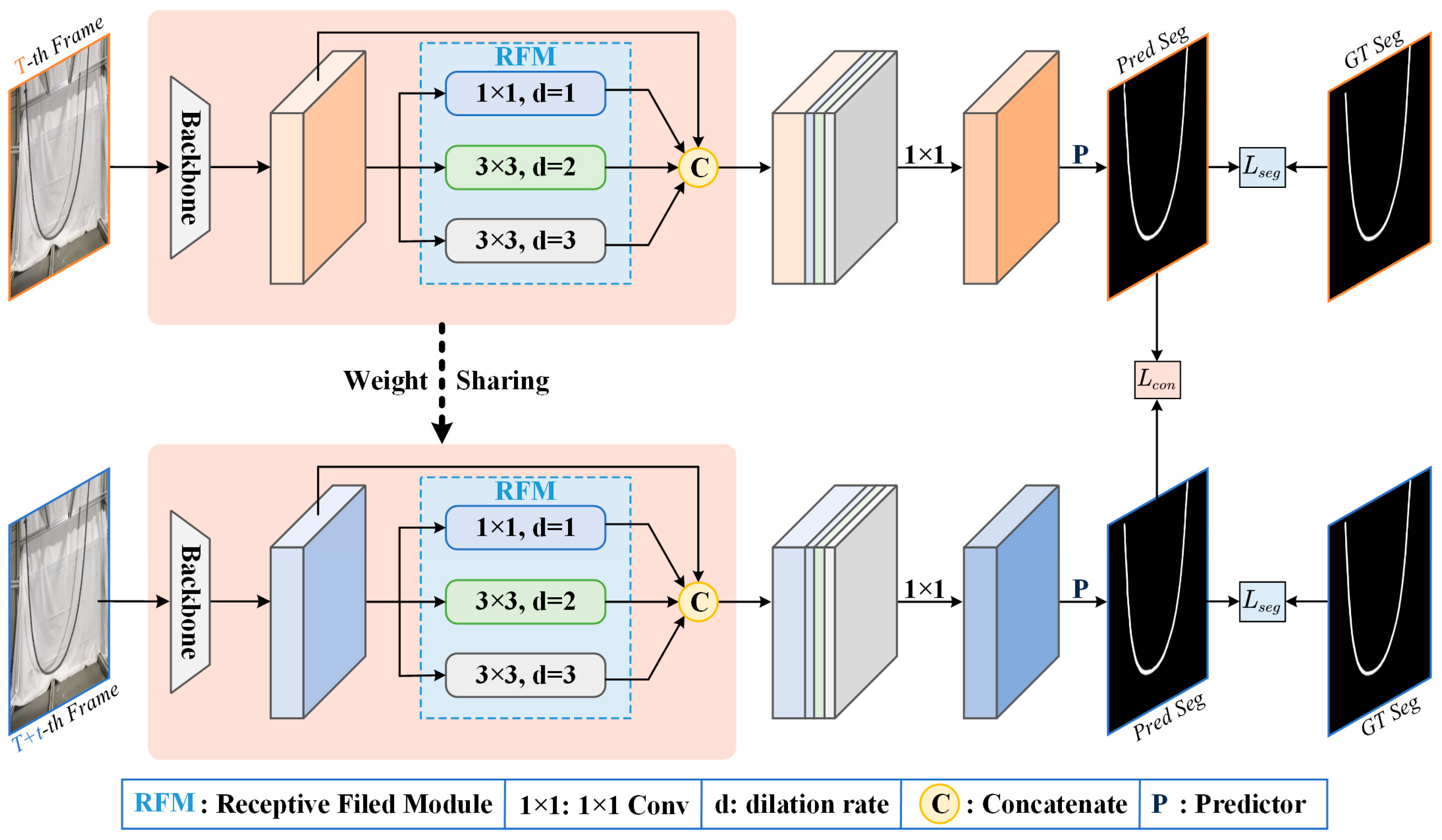
The pivotal step in acquiring the displacement of the tail rope is identifying the rope entity from the background. Naturally, one can draw inspiration from substantial successes of semantic segmentation [27,28,29,30,31,32] and construct a fully convolutional network for tail rope segmentation. In this way, the input videos would be modeled as a sequence of independent frames and processed by the conventional segmentation paradigm, which, unfortunately, would result in a loss of the intrinsic correlations in the temporal dimensions. Hence, we devised a Siamese Segmentation network namely SiamSeg which is demonstrated in Figure 2. It can be seen that our SiamSeg embodies a dual-path pipeline, which is enlightened by the tremendous success in Siamese-based tracking approaches [33,34,35,36].
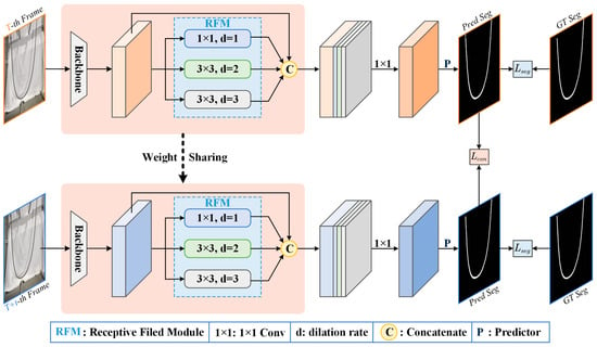
Figure 2.
Overall pipeline of the proposed SiamSeg. The input images are fed into the weight-shared backbone to obtain compact representations. A Receptive Field Module (RFM) is then designed based on dilation convolutions of various dilation rates to expand the receptive field, thereby enabling the holistic segmentation of tail rope. Afterward, a simple predictor is introduced to acquire the binary segmentation mask, and the entire procedure is optimized by the proposed segmentation loss . Moreover, a consistency loss is devised to mine the temporal correlations and guarantee the consistency between the corresponding predictions of two input images.
2.1.1. Feature Extraction
Dual architecture was employed for tail rope segmentation, in which the weights of the backbone part and the proposed Receptive Field Module (RFM) were shared between two parallel branches. Specifically, the powerful residual network [37] was leveraged to serve as the backbone, and the last two subsampling layers in ResNet-50 were dropped to preserve the rope details as much as possible. We were given two input images and corresponding to the T-th and T + t-th frames, respectively, and the spatial size of was , in which and indicate the height and width of the input image, respectively. The corresponding representations from the backbone network were and with the shape . Afterward, an based on dilation convolutions of various dilation rates was installed to expand the receptive field, thereby enabling the holistic segmentation of tail ropes, which can be formulated as follows:
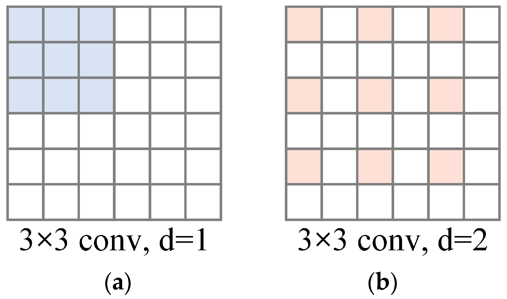
where denotes the Receptive Field Module, while and denote the output of features from RFM. The consideration of introducing RFM is mainly attributed to the elongated structure of the rope, which often poses a challenge where only local regions are correctly segmented. Therefore, an RFM based on the dilation convolution, which is also known as atrous convolution, was constructed [29], thereby capturing long-range dependencies. As shown in Figure 3, the dilation convolution degrades to conventional convolution when the dilation rate is 1 (refer to (a)), while setting the dilation rate at 2 introduces gaps or spaces between the kernel elements, which is referred to as the dilation rate. This condition enlarges the receptive field without increasing the number of parameters.
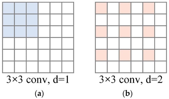
Figure 3.
The dilation convolutions with a kernel size of 3 and a dilation rate of 1 (a) and 2 (b). Notably, the colored blocks represent the sampling locations for convolution.
The output channels of RFM were set as 32 to further reduce the computational overhead. The dilated features were concatenated with the input representations to preserve the structural layouts as follows:
where denotes the concatenation operation. and are the sizes of . Afterward, a convolution with output channels of 256 was utilized to integrate the channel-wise information.
2.1.2. Segmentation Prediction
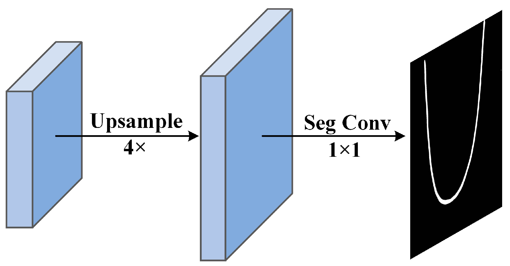
A segmentation predictor was then introduced after obtaining the compact representation of input images to procure the binary masks. Figure 4 illustrates the designed predictor. First, the input features were upsampled with the ratio of 4, and a convolution was then leveraged to obtain the prediction mask. The entire procedure can be described as follows:
where and indicate the segmentation predictor and upsampling, respectively. and represent the predicted binary masks.

Figure 4.
The designed predictor.
2.1.3. Loss Function
Next, the objective functions tailored for the dual-branch SiamSeg were highlighted. The tail rope only occupies a small portion of the image. Therefore, the conventional segmentation loss fails to provide satisfactory results because it cannot handle the imbalance issue. To this end, the following segmentation loss was designed to enable the optimization of the segmentation branch:
where denotes the ground truth binary map, and represents the overall pixels. Meanwhile, indicates the current location. The term refers to the numerical stability. The devised effectively addresses sample imbalance by emphasizing the intersection of positive predictions, ensuring a highly balanced consideration of minority classes in imbalanced scenarios. Moreover, the inherent correlations along the temporal dimension in sequential data can be leveraged to facilitate the recognition of tail ropes. Specifically, the displacement of the ropes shows no discernible variations in a series of images spaced at intervals. A loss function was further devised based on this consensus to guarantee the consistency between the predictions correspond to T-th frame and T + t-th frame, which can be illustrated as follows:
where and represent the predicted foreground regions in the binary segmentation maps. and denote the intersection and union operations on two respective regions, respectively, while the term indicates the temporal interval between two input video frames.
2.2. Pixel-Wise Displacement
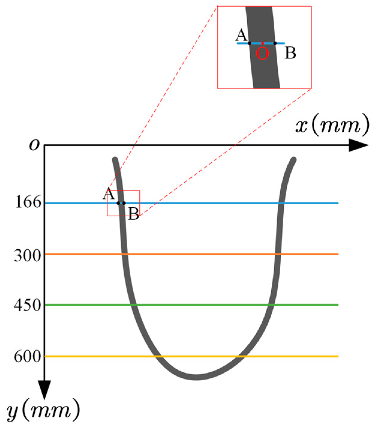
As shown in Figure 5, in the pixel coordinate system, taking the time interval as an example, the point on the centerline of the rope was denoted as , and the coordinates of the corresponding edge points on both sides were and . The coordinates of point were denoted as , and the coordinates of point were denoted as . During rope movement, at time , the coordinates of points and in the image were and , respectively, while the coordinates of point were denoted as . At time , the coordinates of points and in the image were and , respectively, and the coordinates of point were denoted as . Therefore, the displacement of the tail rope at this monitoring point within the time interval can be obtained as follows:

Figure 5.
Calculation of pixelwise displacement of tail ropes. Different colored lines represent different monitoring locations, corresponding to different pixel positions.
3. Experiment and Analysis
3.1. Data Acquisition
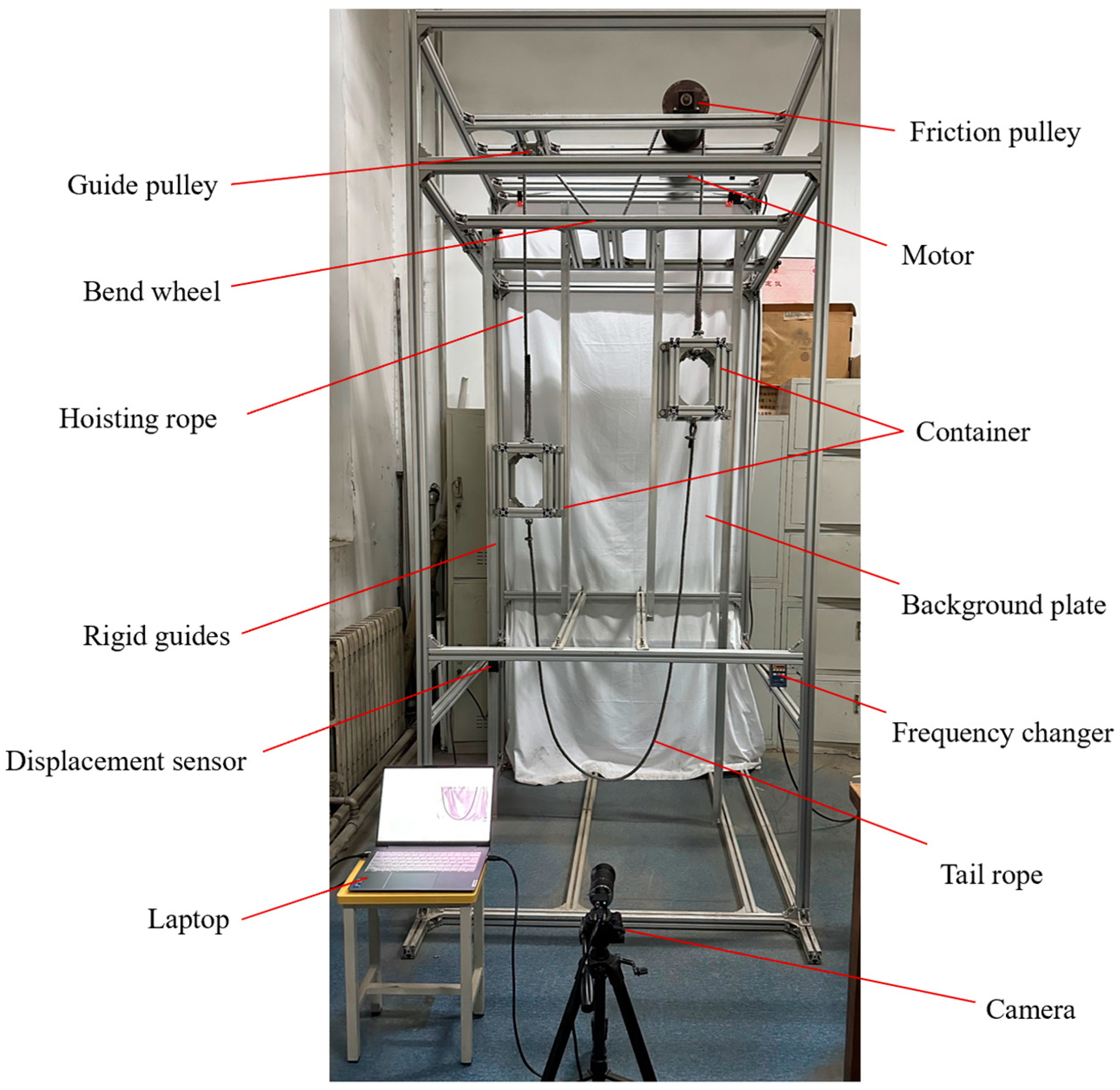
Obtaining the real video of the tail rope during operation is difficult due to the particularity and complexity of the underground environment. An experimental platform was designed and built in accordance with the principle of hoisting to verify the effectiveness of this method. In the traditional friction hoisting system, the tail rope is freely suspended, and its head end and the tail end move with the container. When the system is running, the friction pulley drives the movement of the hoisting rope to realize the reciprocating movement of the hoisting container. When the hoisting container moves on the rigid guide, the tail rope is freely suspended and is naturally hung down by gravity. The experimental platform for the lateral swing of the hoist rope was established through the appropriate simplification of irrelevant variables. This platform mainly comprised the experimental support, driving motor, frequency converter, friction pulley, guide pulley, hoisting rope, container, tail rope, rigid guide, counterweight equipment, camera, tripod, displacement sensor, and light source. Figure 6 shows the overall experimental device.
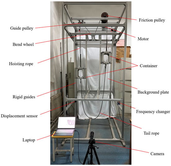
Figure 6.
Experimental setup.
The video of the tail rope swing is shot by the camera, and the video information is transmitted to the computer. The swing displacement of the tail rope during operation is obtained after calculation and analysis by the image processing software of the computer, and the real-time measurement of the fixed-point and multipoint dynamic displacement of the tail rope is realized. The laser-ranging module sensor S1-400 (TTL) was selected in this study to verify the accuracy of the experimental results. The measurement error of this sensor is less than 3% with a FOV = 24°. The sensor communicates with the computer through the TTL serial port and outputs the swing displacement in real time. The sensor is arranged on the left side of the experimental platform, which can collect the real-time swing displacement of the tail rope at the monitoring position during the movement. Compared with the measurement results proposed in this study, the obtained data of the sensor are used to verify the effectiveness of this method. In the experiment, the resolution of the video recorded by the camera is 1920 × 1080, and the frame rate of the video is 30 fps. A total of 48 videos were recorded in the experiment, revealing a total duration of 373 s, of which 24 videos were used for training, 10 videos were for verification, and the remaining 14 videos were used for testing.
3.2. Camera Calibration
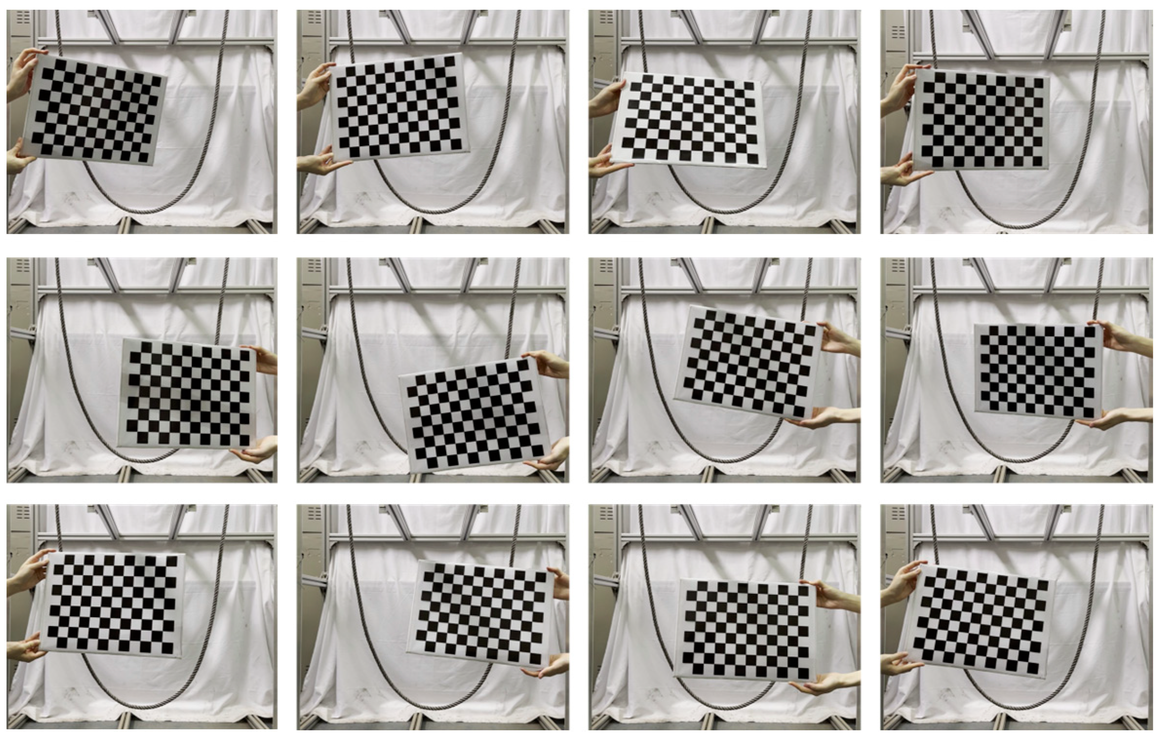
Establishing the relationship between the camera and real-world measurements is necessary to build a bridge between them. Camera calibration can convert image information into world information. The internal parameter matrix, external parameter matrix, and distortion parameters of the camera can be determined through calibration. The plane calibration method proposed by Zhang Z Y [38] is one of the most widely used and practical calibration methods. This camera calibration method uses a square checkerboard with known parameters. As shown in Figure 7, the mutual positions and sizes of the black cubes on the calibration board are known. Assuming that the origin of the world coordinate system is the top left corner point on the chessboard, the world coordinate system will also change during chessboard rotation. The checkerboard images with different positions and angles are collected, and the rotation and translation matrices of each image are expressed as and , respectively, where . In each picture, corner points are selected and calibrated. The world coordinate of the corner point on each picture is a fixed value, where . The focal length of the camera is fixed in the process of image acquisition. Therefore, the internal parameter matrix of the camera is a constant matrix. According to the pinhole imaging model, the following can be obtained:
where denotes the coordinates projected by the -th corner point of the -th calibration image on the image plane; is a scale factor; and , and represent the internal reference, rotation, and translation matrices, respectively, of the -th calibration image, which are collectively referred to as the parameters of the camera.
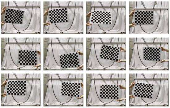
Figure 7.
Partial calibration images.
With the known actual pixel coordinate of corner points, the parameters of the camera can be solved by the optimized objective equation :
According to the calibration principle, the calibration method proposed by Zhang needs multiple calibration images, and more than 10 calibration images are generally used in practical applications to ensure the calibration accuracy. In this study, a chessboard calibration board with a single cell size of was adopted, including 12 and 9 cells in the horizontal and vertical directions, respectively. By adjusting the position and angle of the calibration board, several pictures were taken, and partial calibration images are shown in Figure 7 below.
Figure 8 shows the relative positions of the camera and the calibration board. The maximum calibration error of the camera is 0.16, and the average error is controlled at 0.13, which is small, meeting the relevant requirements.
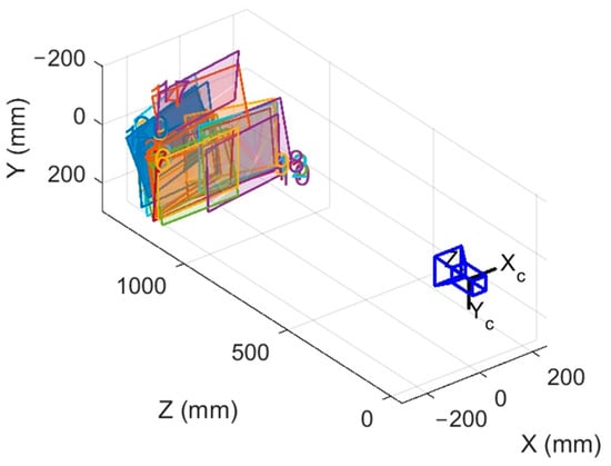
Figure 8.
Relative position between the camera and the calibration board.
3.3. Image Processing
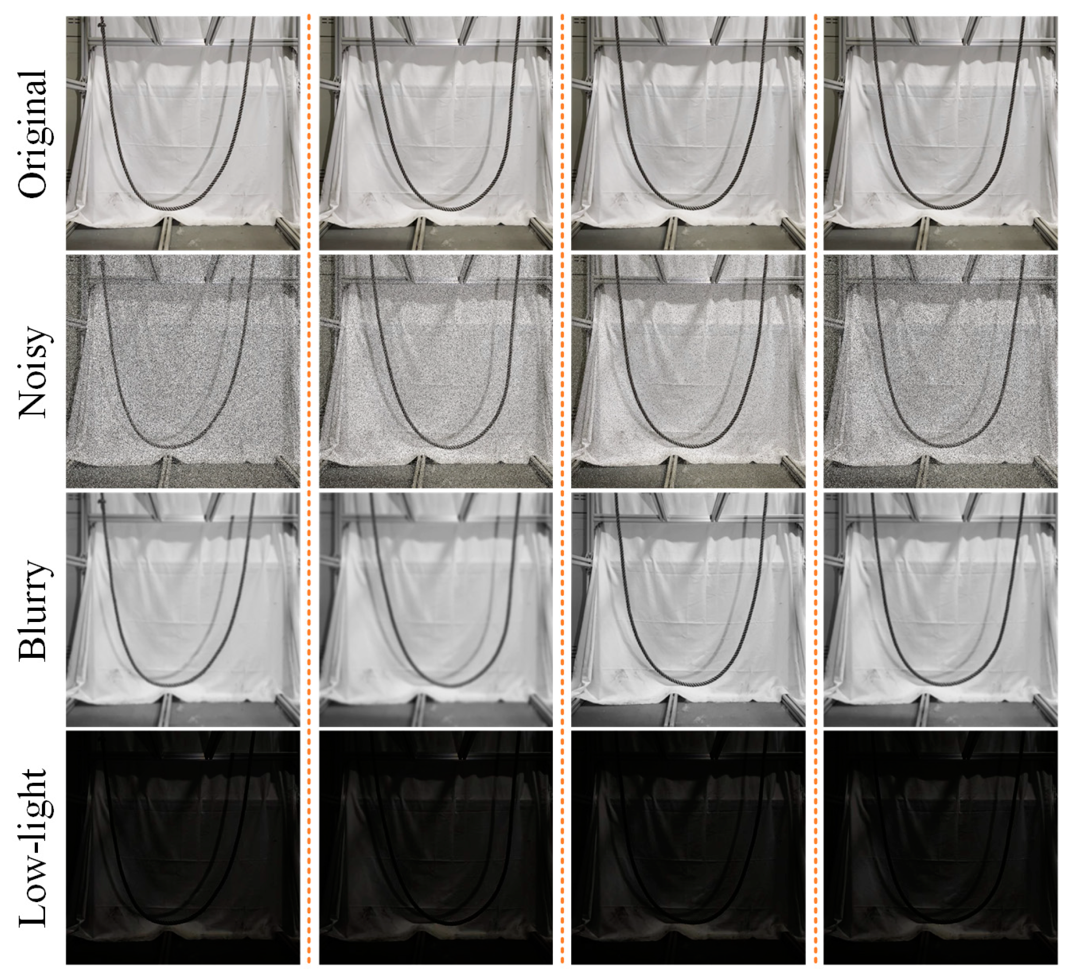
The images are captured from the simulation platform, which inevitably introduces data redundancy to the table due to the single scenario. Worse still, this condition induces overfitting and substantially hinders segmentation performance. To this end, the input data are first augmented to enhance diversity. Specifically, noise is added or blurred in a training image. Moreover, a low-light strategy is installed to the input images to adapt to the underground environment effectively. Some example images processed by these augmentation schemes are intuitively visualized in Figure 9.
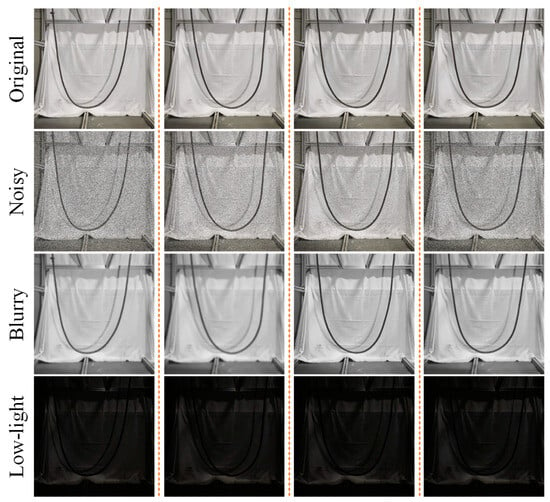
Figure 9.
Images processed by the augmentation strategies, in which Noisy indicates the images added with noises, while Blurry represents the images processed by Gaussian blur. Low-light denotes the images after low-light enhancement.
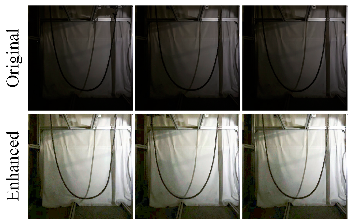
Furthermore, the contrast settings are varied to obtain various data that closely simulate real-world environments as much as possible. As shown in Figure 10, these images will be enhanced during training and inference. Using the MSRCP (Multi-Scale Retinex with Color Preservation) algorithm, which combines the multi-scale Retinex algorithm and color preservation techniques, enhances the details and contrast of low-light images while maintaining the natural colors of the images.

Figure 10.
Images captured under low-light conditions (Original) and the corresponding enhanced images (Enhanced).
The aforementioned processing considerably improves the diversity and variability of the input data for the subsequent segmentation model and, most importantly, contributes to its robustness in terms of the potential application scenarios.
3.4. Model Evaluation and Experimental Results
This section describes the results of the proposed SiamSeg on the constructed tail rope dataset. Moreover, some ablation studies regarding optimal setups in the proposed approach are provided.
3.4.1. Evaluation Metrics
The mean Intersection over Union (mIoU) and F1 score are leveraged to evaluate the effectiveness of the proposed method on the tail rope segmentation task. is defined as follows:
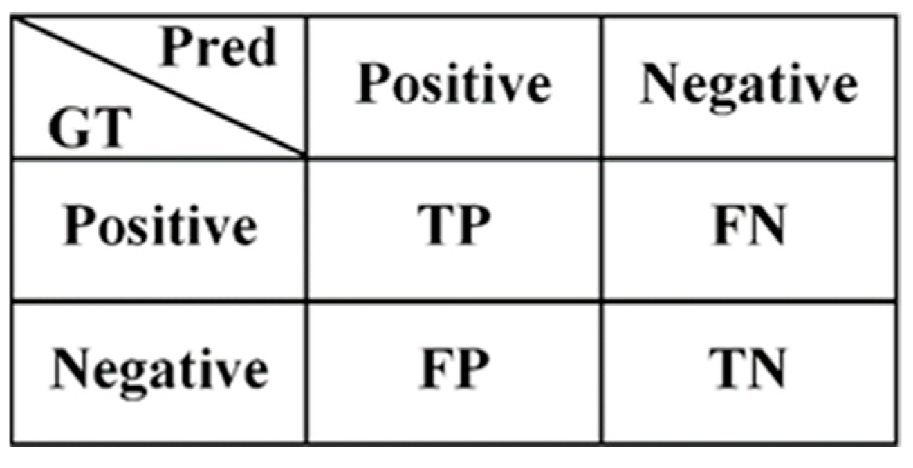
where denotes the number of foreground categories, while , , and represent True Positive, False Positive, and False Negative, respectively. Figure 11 presents additional details.
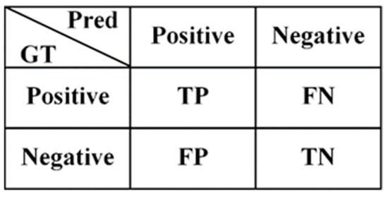
Figure 11.
Definition of TP, FP, and FN, where GT denotes the ground truth pixel annotation, while Pred indicates the predicted segmentation map.
The score, also known as the F1 measure, is a metric commonly used to evaluate the performance of classification models, including binary semantic segmentation tasks. It is the harmonic mean of precision and recall and is calculated using the following formula:
where and can be respectively formulated as follows:
3.4.2. Experimental Results
SiamSeg and previous segmentation approaches were evaluated on the test set, and the results are shown in Table 1. The table reveals that the classical segmentation approaches, including GrabCut and Otsu [39], perform catastrophically on the tail rope segmentation task. GrabCut and Otsu are speculated to rely on handcrafted features and may struggle to capture complex patterns and nuanced details present in images, especially in scenarios with intricate structures such as ropes. Moreover, rope segmentation often involves dealing with variations in lighting, viewpoint, and occlusions, which pose considerable challenges to these traditional algorithms with fixed feature representations. Meanwhile, Deeplab [29], EncNet [30], and LETNet [31] show clear predominance to the classical approaches. To be specific, DeepLab leads the other solutions by a large margin due to the exploitation of contextual cues. EncNet uses the Context Encoding Module to aggregate class-specific context information, enhancing the model’s ability to make more accurate segmentation decisions. LETNet effectively combines U-shaped CNNs with transformers, leveraging the advantages of CNNs in local feature extraction and transformers in capturing global information. Unsurprisingly, SiamSeg achieves the best performance, demonstrating the effectiveness of the proposed segmentation framework for tail ropes. Furthermore, the shared backbone integrated with the designed RFM enables the powerful and discriminative representation of rope regions. Moreover, the Siamese structure, along with the consistency loss, efficiently leverages the temporal correlations inherent in the input data.

Table 1.
Performance comparison between the proposed SiamSeg and other representative segmentation methods on the test set.
As previously reported, SiamSeg collects two frames with an interval of as input, and this interval also contributes to the consistency loss . Considering , various setups are then investigated to determine the optimal setting. Table 2 shows the results.
Table 2.
Effect of various setups of t on the segmentation performance. The best result is in bold.
When is substantially small, the consistency loss has minimal effects due to the absence of discernible displacement between the two input images. Moreover, an excessively large choice of fails to yield a satisfactory performance due to the possible existence of large deformations. Thus, enforcing the alignment of the predictions of two sibling branches is inappropriate and suboptimal in this scenario. Hence, is set at 9 based on the experiments.
3.4.3. Segmentation Result Visualization
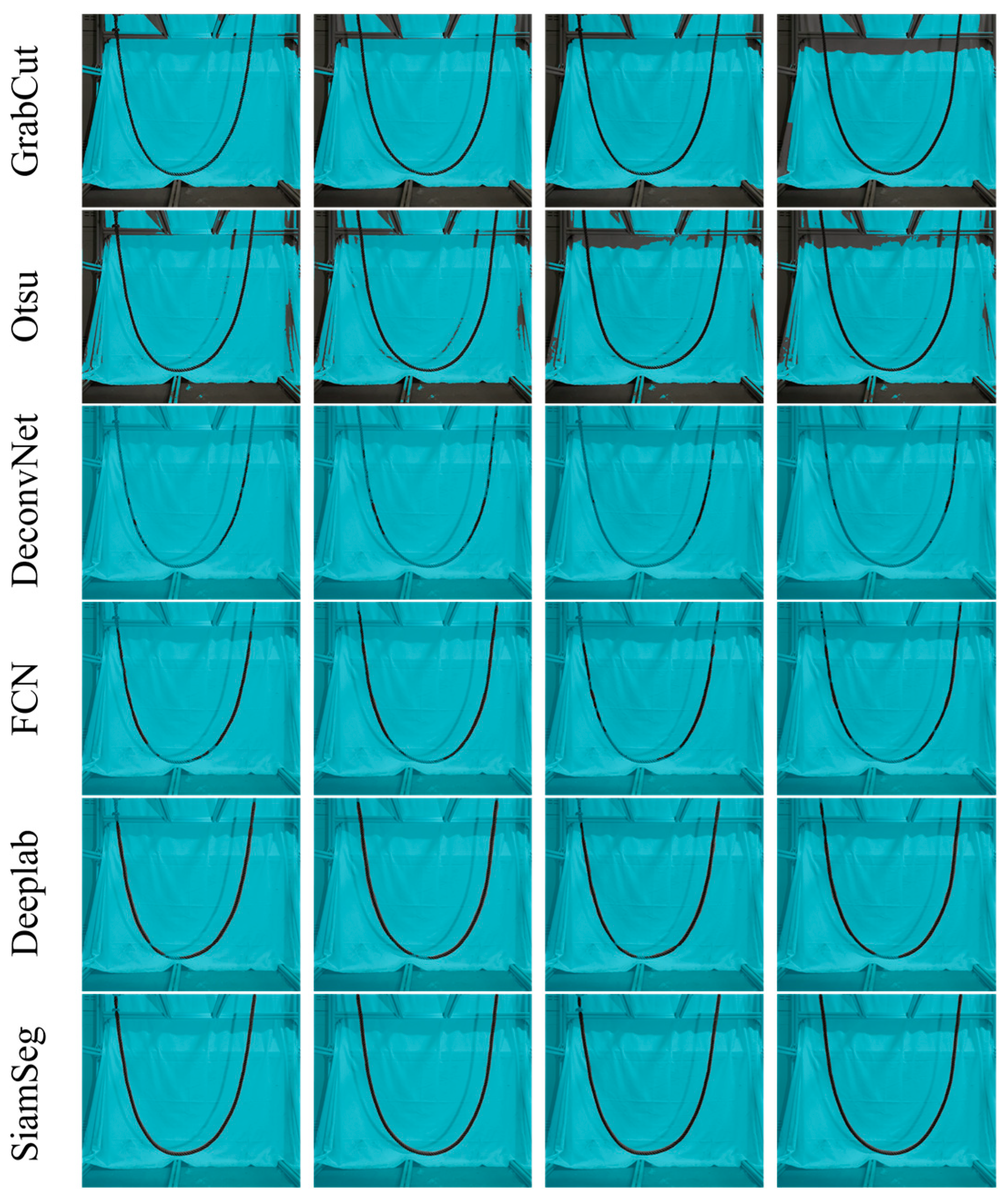
Figure 12 also visualizes the segmentation results of each method on the test set, thereby intuitively exhibiting the effectiveness of the proposed approach in handling the elongated tail ropes.
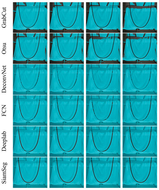
Figure 12.
Segmentation visualization of each method on the test set.
3.4.4. Results Analysis
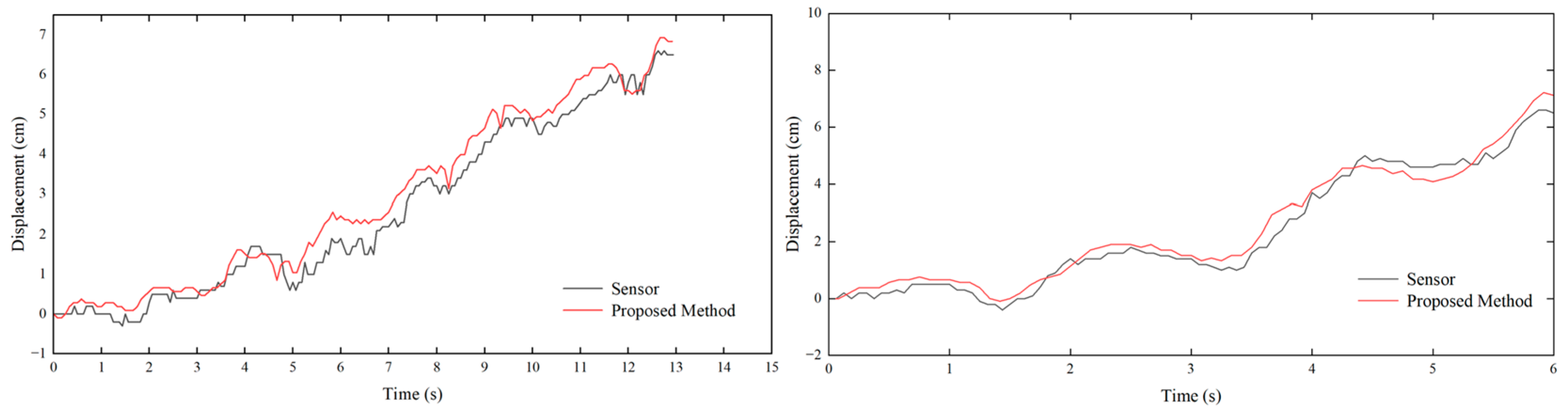
The tail rope in operation was monitored simultaneously by the camera and sensor to verify the accuracy and feasibility of the visual measurement method proposed in this study. Using the method described in Section 2, the swing displacement of the tail rope could be extracted from the camera-captured video and compared with the data measured by the sensor. Figure 13 displays the randomly selected two groups of data.
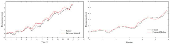
Figure 13.
Comparison between the measurement results obtained from the proposed method and those from the sensor.
When evaluating the measurement results, the visual measurement result is denoted as , the sensor-measured result is , and the absolute error is computed as follows:
The absolute error of the first group of experimental results was calculated as 0.33 cm, and the relative error of measurement was approximately 2.6%. In the second group, the two figures were 0.27 cm and approximately 2.5%, respectively. The swing displacement result measured by the proposed visual method fell into the allowable range of errors.
Two parameters, namely hoisting load and operating speed, were mainly adjusted to simulate the swing of the tail rope as much as possible in the laboratory. Specifically, three different hoisting loads (0, 5, and 10 kg) were experimentally set. The operating speed was adjusted mainly by changing the rotating speed of the motor to 14, 28, 42, and 56 r/min. Table 3 lists the parameter settings.
Table 3.
Experimental parameter settings.
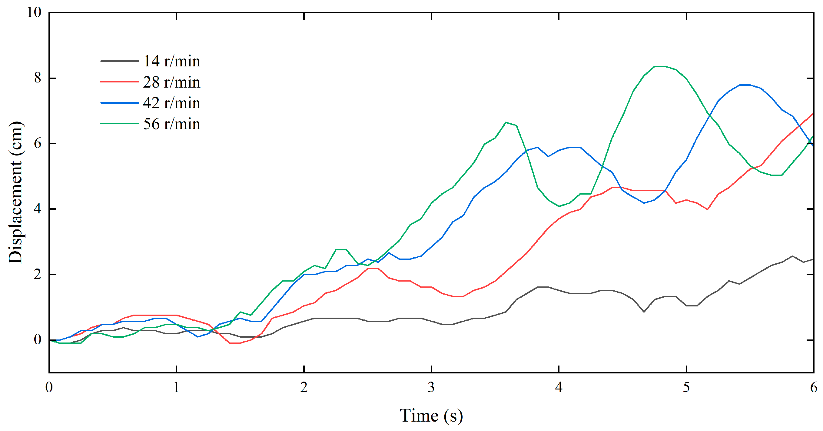
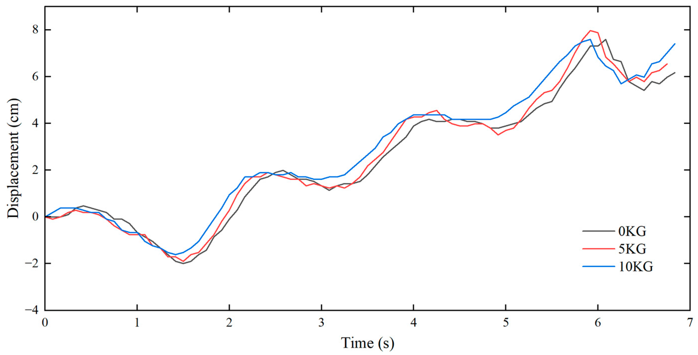
As shown in Figure 14, the displacements of the tail rope at the same monitoring point and load condition but at different operating speeds could be acquired through the above experiment. The figure revealed that as the operating speed was accelerated, the peak and valley values of the swing amplitude at the same monitoring position grew and appeared earlier. Figure 15 displays the displacement comparison of the tail rope at the same monitoring point and operating speed but under different load conditions. Notably, at the same operating speed, the swing displacements at the same monitoring point and different load conditions were largely consistent.
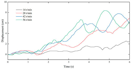
Figure 14.
Comparison of displacements under different operating speeds (example with 0 kg Load).
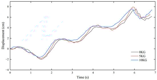
Figure 15.
Comparison of displacements under different loading conditions (example with 28 r/min).
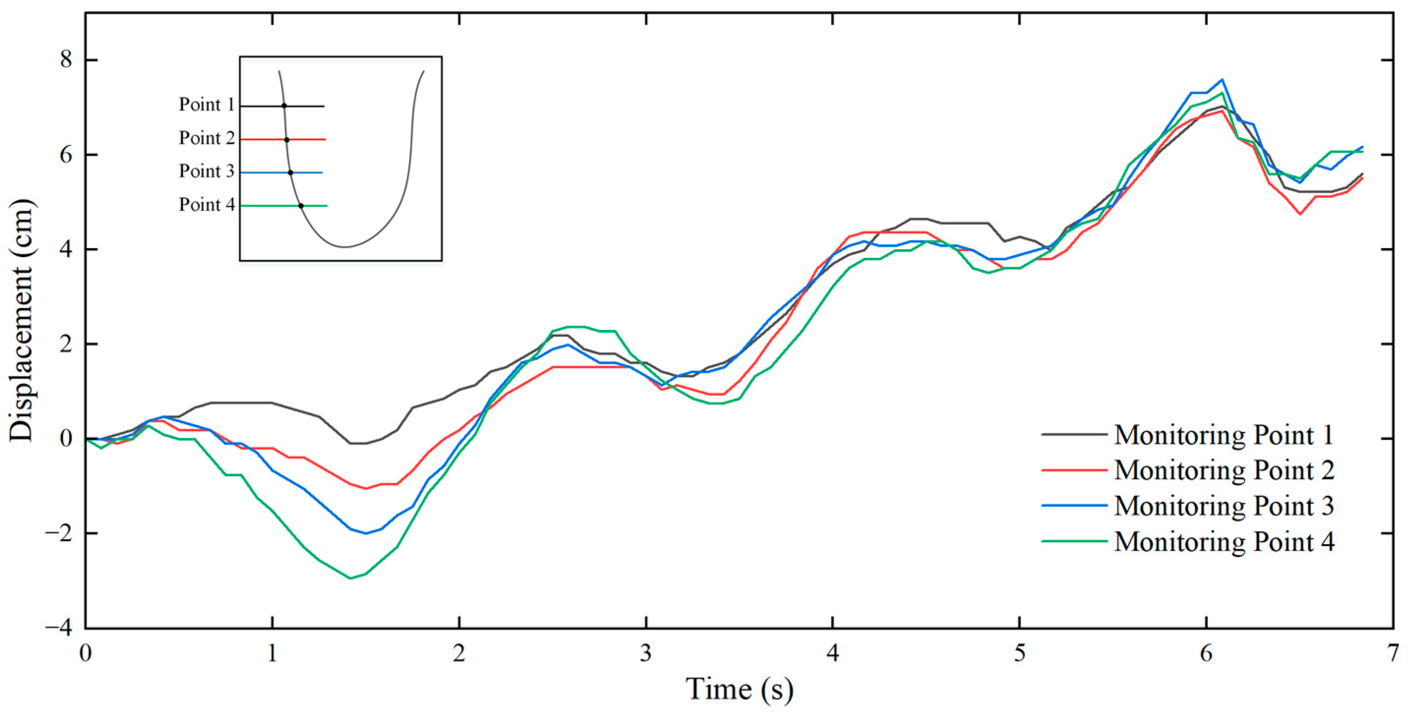
Under the same load and operating speed, four different monitoring points of the tail rope were selected, at which the lateral swing displacements were measured, as shown in Figure 16. Point 4 was closer to the tail ring, and the peak and valley values of swing displacement were the maximum and appeared early. The swing amplitude at other monitoring points decreased successively as the distance from the bottom of the tail rope increased. The underground tail rope was excessively long as a one-dimensional continuous moving body. Thus, the selection of its monitoring area is also crucial for the monitoring result. The above experimental results indicate that the swing amplitude at the tail ring is relatively large. Hence, this position can serve as the best area for visual monitoring, which is convenient for subsequent health monitoring and provides an additional guarantee for the safe operation of the hoisting system.
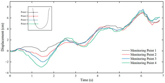
Figure 16.
Comparison of displacements at different monitoring points.
4. Conclusions
In this study, a vision-based target-free online monitoring method for the lateral swing of tail ropes was designed to address the monitoring problem in the lateral swing of flexible axial moving objects such as tail ropes, combined with deep learning. This method captures the video of tail rope operation and inputs the video data into the designed network model, realizing pixel-level displacement recognition. Finally, the lateral swing displacement of the tail rope in the real world is acquired through the transformation of pixel and world coordinates. The main conclusions are drawn as follows:
(1) In this study, a measurement model for the lateral swing displacement of the tail rope was designed. A dual-branch SiamSeg was adopted, to which an RFM module was added. Thus, the receptive field was enhanced without adding model parameters, and the feature extraction capability of the model was strengthened. The main and auxiliary loss functions with a time sequence consistency constraint were designed based on the time sequence of video data to effectively identify the tail rope accounting for a substantially small proportion in the video frame. An experimental platform was established for model training to simulate the swing of the tail rope. In this study, the mIoU and F1 score were chosen as the evaluation indicators, which were shown to be 95.7% and 90.2%, respectively, based on the dataset, both being higher than those obtained by the other comparative methods. The visualization results revealed that this model overcomes the susceptibility of the shadow and achieves a better segmentation effect than other methods.
(2) The results obtained by the proposed method were compared with sensor-measured results, and the absolute error ranged from 2 mm to 3 mm, indicating that this method can meet the engineering demand for the lateral swing measurement of tail ropes. The tail rope swing under different underground conditions was simulated via the experimental platform, and some swing laws of the tail rope were summarized using the proposed method. The length of the tail rope in the deep well is substantially greater than that on the experimental platform. Thus, the monitoring result will be affected by the selection of the monitoring area. Therefore, the optimal monitoring area can be set at the tail rope loop according to the analysis of the experimental results.
Overall, the proposed method in this study can provide reliable data on tail rope swing displacement, supplying a basis for further monitoring the health status of the hoisting system and ensuring its safe operation. This method provides a new solution to underground monitoring of the motion state of wire ropes in the hoisting system. However, some other challenges are still encountered in the follow-up research, such as the impact of underground vibration and water mist on the video frame. On the premise of ensuring precision, a lightweight network model should be established to adapt to the terminal resource limitations.
Author Contributions
Software, validation, investigation, and writing—original draft preparation: X.Z. Conceptualization and funding acquisition: G.M. Methodology and writing—review and editing: A.W. All authors have read and agreed to the published version of the manuscript.
Funding
This research was supported by the National Natural Science Foundation of China, grant number U1361127.
Data Availability Statement
Data can be made available upon reasonable request.
Conflicts of Interest
The authors declare no conflicts of interest.
References
- Wang, Y.; Wang, C.; Feng, Y.; Dai, B.; Wu, G. Application and Analyzation of the Vision-Based Structure Model Displacement Measuring Method in Cassette Structure Shaking Table Experiment. Adv. Civ. Eng. 2020, 2020, 8869935. [Google Scholar]
- Manikandan, K.G.; Pannirselvam, K.; Kenned, J.J.; Kumar, C.S. Investigations on suitability of MEMS based accelerometer for vibration measurements. Mater. Today Proc. 2021, 45, 6183–6192. [Google Scholar] [CrossRef]
- Liu, F.; Gao, S.; Chang, S. Displacement estimation from measured acceleration for fixed offshore structures. Appl. Ocean. Res. 2021, 113, 102741. [Google Scholar] [CrossRef]
- Zhu, H.; Gao, K.; Xia, Y.; Gao, F.; Weng, S.; Sun, Y.; Hu, Q. Multi-rate data fusion for dynamic displacement measurement of beam-like supertall structures using acceleration and strain sensors. Struct. Health Monit. 2020, 19, 520–536. [Google Scholar] [CrossRef]
- Kou, B.F.; Liu, Q.Z.; Liu, C.Y.; Liang, Q. Characteristic research on the transverse vibrations of wire rope during the operation of mine flexible hoisting system. J. China Coal Soc. 2015, 40, 1194–1198. [Google Scholar]
- Park, H.S.; Kim, J.M.; Choi, S.W.; Kim, Y. A wireless laser displacement sensor node for structural health monitoring. Sensors 2013, 13, 13204–13216. [Google Scholar] [CrossRef]
- Nassif, H.H.; Gindy, M.; Davis, J. Comparison of laser Doppler vibrometer with contact sensors for monitoring bridge deflection and vibration. Ndt E Int. 2005, 38, 213–218. [Google Scholar] [CrossRef]
- Kamal, A.M.; Hemel, S.H.; Ahmad, M.U. Comparison of linear displacement measurements between a mems accelerometer and Hc-Sr04 low-cost ultrasonic sensor. In Proceedings of the 2019 1st International Conference on Advances in Science, Engineering and Robotics Technology (ICASERT), Dhaka, Bangladesh, 3–5 May 2019. [Google Scholar]
- Xia, W.H.; Ling, M.S. Non-contact displacement measurement based on magnetoresistive sensor. Foreign Electron. Meas. Technol. 2010, 28, 28–30. [Google Scholar]
- Lee, C.H.; Hong, S.; Kim, H.W.; Kim, S.S. A comparative study on effective dynamic modeling methods for flexible pipe. J. Mech. Sci. Technol. 2015, 29, 2721–2727. [Google Scholar] [CrossRef]
- Feng, D.; Feng, M.Q. Computer vision for SHM of civil infrastructure: From dynamic response measurement to damage detection–A review. Eng. Struct. 2018, 156, 105–117. [Google Scholar] [CrossRef]
- Tan, Q.; Kou, Y.; Miao, J.; Liu, S.; Chai, B. A model of diameter measurement based on the machine vision. Symmetry 2021, 13, 187. [Google Scholar] [CrossRef]
- Li, B. Research on geometric dimension measurement system of shaft parts based on machine vision. EURASIP J. Image Vide. 2018, 2018, 101. [Google Scholar] [CrossRef]
- Marrable, D.; Tippaya, S.; Barker, K.; Harvey, E.; Bierwagen, S.L.; Wyatt, M.; Bainbridge, S.; Stowar, M. Generalised deep learning model for semi-automated length measurement of fish in stereo-BRUVS. Front. Mar. Sci. 2023, 10, 1171625. [Google Scholar] [CrossRef]
- Kutlu, I.; Soyluk, A. A comparative approach to using photogrammetry in the structural analysis of historical buildings. Ain Shams Eng. J. 2024, 15, 102298. [Google Scholar] [CrossRef]
- Khuc, T.; Nguyen, T.A.; Dao, H.; Catbas, F.N. Swaying displacement measurement for structural monitoring using computer vision and an unmanned aerial vehicle. Measurement 2020, 159, 107769. [Google Scholar] [CrossRef]
- Xu, Y.; Zhang, J.; Brownjohn, J. An accurate and distraction-free vision-based structural displacement measurement method integrating Siamese network based tracker and correlation-based template matching. Measurement 2021, 179, 109506. [Google Scholar] [CrossRef]
- Lee, G.; Kim, S.; Ahn, S.; Kim, H.K.; Yoon, H. Vision-based cable displacement measurement using side view video. Sensors 2022, 22, 962. [Google Scholar] [CrossRef]
- Fukuda, Y.; Feng, M.Q.; Shinozuka, M. Cost-effective vision-based system for monitoring dynamic response of civil engineering structures. Struct. Control Health Monit. 2010, 17, 918–936. [Google Scholar] [CrossRef]
- Wahbeh, A.M.; Caffrey, J.P.; Masri, S.F. A vision-based approach for the direct measurement of displacements in vibrating systems. Smart Mater. Struct. 2003, 12, 785–794. [Google Scholar] [CrossRef]
- Chen, C.C.; Wu, W.H.; Tseng, H.Z.; Chen, C.H.; Lai, G. Application of digital photogrammetry techniques in identifying the mode shape ratios of stay cables with multiple camcorders. Measurement 2015, 75, 134–146. [Google Scholar] [CrossRef]
- Bhowmick, S.; Nagarajaiah, S.; Lai, Z. Measurement of full-field displacement time history of a vibrating continuous edge from video. Mech. Syst. Signal Process. 2020, 144, 106847. [Google Scholar] [CrossRef]
- Xu, Y.; Brownjohn, J.; Kong, D. A non-contact vision-based system for multipoint displacement monitoring in a cable-stayed footbridge. Struct. Control Health Monit. 2018, 25, e2155. [Google Scholar] [CrossRef]
- Won, J.; Park, J.W.; Park, K.; Yoon, H.; Moon, D.S. Non-target structural displacement measurement using reference frame-based deepflow. Sensors 2019, 19, 2992. [Google Scholar] [CrossRef]
- Yu, S.; Zhang, J.; Su, Z.; Jiang, P. Fast and robust vision-based cable force monitoring method free from environmental disturbances. Mech. Syst. Signal Process. 2023, 201, 110617. [Google Scholar] [CrossRef]
- Caetano, E.; Silva, S.; Bateira, J. Application of a vision system to the monitoring of cable structures. In Proceedings of the Seventh International Symposium on Cable Dynamics, Vienna, Austria, 10–13 December 2007. [Google Scholar]
- Long, J.; Shelhamer, E.; Darrell, T. Fully convolutional networks for semantic segmentation. In Proceedings of the IEEE Conference on Computer Vision and Pattern Recognition, Boston, MA, USA, 7–12 June 2015. [Google Scholar]
- Noh, H.; Hong, S.; Han, B. Learning deconvolution network for semantic segmentation. In Proceedings of the IEEE International Conference on Computer Vision, Santiago, Chile, 7–13 December 2015. [Google Scholar]
- Chen, L.C.; Papandreou, G.; Kokkinos, I.; Murphy, K.; Yuille, A.L. Deeplab: Semantic image segmentation with deep convolutional nets, atrous convolution, and fully connected crfs. IEEE Trans. Pattern Anal. Mach. Intell. 2017, 40, 834–848. [Google Scholar] [CrossRef]
- Zhang, H.; Dana, K.; Shi, J.; Zhang, Z.; Wang, X.; Tyagi, A.; Agrawal, A. Context encoding for semantic segmentation. In Proceedings of the IEEE Conference on Computer Vision and Pattern Recognition, Salt Lake City, UT, USA, 18–22 June 2018. [Google Scholar]
- Xu, G.; Li, J.; Gao, G.; Lu, H.; Yang, J.; Yue, D. Lightweight real-time semantic segmentation network with efficient transformer and CNN. IEEE Trans. Intell. Transp. Syst. 2023, 24, 15897–15906. [Google Scholar] [CrossRef]
- Guo, B.; Wang, Y.; Zhen, S.; Yu, R.; Su, Z. SPEED: Semantic prior and extremely efficient dilated convolution network for real-time metal surface defects detection. IEEE Trans. Ind. Inform. 2023, 19, 11380–11390. [Google Scholar] [CrossRef]
- Bertinetto, L.; Valmadre, J.; Henriques, J.F.; Vedaldi, A.; Torr, P.H. Fully-convolutional siamese networks for object tracking. In Proceedings of the Computer Vision–ECCV 2016 Workshops, Proceedings of the European Conference on Computer Vision, Amsterdam, The Netherlands, 8–16 October 2016; Hua, G., Jégou, H., Eds.; Springer: Berlin/Heidelberg, Germany, 2016; pp. 850–865. [Google Scholar]
- Yu, Y.; Xiong, Y.; Huang, W.; Scott, M.R. Deformable siamese attention networks for visual object tracking. In Proceedings of the IEEE/CVF Conference on Computer Vision and Pattern Recognition, Seattle, WA, USA, 13–19 June 2020. [Google Scholar]
- Li, B.; Wu, W.; Wang, Q.; Zhang, F.; Xing, J.; Yan, J. Siamrpn++: Evolution of siamese visual tracking with very deep networks. In Proceedings of the IEEE/CVF Conference on Computer Vision and Pattern Recognition, Long Beach, CA, USA, 15–20 June 2019. [Google Scholar]
- Hu, W.; Wang, Q.; Zhang, L.; Bertinetto, L.; Torr, P.H. Siammask: A framework for fast online object tracking and segmentation. IEEE Trans. Pattern Anal. Mach. Intell. 2023, 45, 3072–3089. [Google Scholar]
- He, K.; Zhang, X.; Ren, S.; Sun, J. Deep residual learning for image recognition. In Proceedings of the IEEE Conference on Computer Vision and Pattern Recognition, Las Vegas, NV, USA, 27–30 June 2016. [Google Scholar]
- Zhang, Z. A flexible new technique for camera calibration. IEEE Trans. Pattern Anal. Mach. Intell. 2000, 22, 1330–1334. [Google Scholar] [CrossRef]
- Otsu, N. A threshold selection method from gray-level histograms. Automatica 1975, 11, 23–27. [Google Scholar] [CrossRef]

Disclaimer/Publisher’s Note: The statements, opinions and data contained in all publications are solely those of the individual author(s) and contributor(s) and not of MDPI and/or the editor(s). MDPI and/or the editor(s) disclaim responsibility for any injury to people or property resulting from any ideas, methods, instructions or products referred to in the content. |
© 2024 by the authors. Licensee MDPI, Basel, Switzerland. This article is an open access article distributed under the terms and conditions of the Creative Commons Attribution (CC BY) license (https://creativecommons.org/licenses/by/4.0/).