Abstract
This paper presents an enhanced Faster R-CNN model for detecting surface defects in resistance welding spots, improving both efficiency and accuracy for body-in-white quality monitoring. Key innovations include using high-confidence anchor boxes from the RPN network to locate welding spots, using the SmoothL1 loss function, and applying Fast R-CNN to classify detected defects. Additionally, a new pruning model is introduced, reducing unnecessary layers and parameters in the neural network, leading to faster processing times without sacrificing accuracy. Tests show that the model achieves over 90% accuracy and recall, processing each image in about 15 ms, meeting industrial requirements for welding spot inspection.
1. Introduction
Welding spot quality is a very crucial factor that affects the hardware reliability of auto-body manufacturing. In the body-in-white (BIW) production phase, the resistance spot welding (RSW) method is widely used. A lot of traditional image processing techniques were adopted in a previous work [1]. However, these methods cannot work well with the influence of environmental factors such as vibration, dust, and lightness, which all usually appear during the inspection [2]. Therefore, the manual visual inspection method is still widely used for surface defect inspection in many workshops nowadays.
At present, the quality inspection of BIW welds mainly includes two types of methods: non-visual and visual inspection [3]. These methods can be divided into non-destructive testing technology and destructive testing technology. Non-visual methods mainly include ultrasonic testing, X-ray inspection, dynamic resistance monitoring, tensile testing, and electromagnetic testing [4].
Ultrasonic non-destructive testing (NDT) [5]: Mirmahdi et al. [6] provided a comprehensive review of ultrasonic testing for resistance spot welding, highlighting its effectiveness in determining the integrity of welding spots. Similarly, some researchers [7,8] explored the use of ultrasonic methods to assess weld quality, demonstrating its accuracy in identifying internal inconsistencies.
X-ray imaging technique: Juengert et al. [9] employed X-ray technology to inspect automotive spot welds, showcasing its ability to reveal internal defects that may compromise weld strength. Similarly, Maeda et al. [10] investigated X-ray inspection of aluminum alloy welds, confirming its capability in the non-invasive evaluation of weld quality.
Dynamic resistance monitoring: Butsykin et al. [11] explored the application of dynamic resistance in real-time quality evaluation of resistance spot welds, suggesting that fluctuations in resistance provide key indicators of weld formation. Wang [12] developed this approach, demonstrating its effectiveness in detecting weld faults through real-time monitoring of resistance signals.
Tensile testing: Safari. [13] investigated the tensile-shear performance of spot welds, providing insights into the relationship between mechanical properties and weld quality. Radakovic et al. [14] examined failure modes in tensile testing, offering a detailed analysis of the impact of weld conditions on shear strength and failure behavior.
Electromagnetic testing is also a non-contact method that evaluates the electromagnetic properties of welds to detect imperfections. Tsukada et al. [15] utilized magnetic flux leakage testing to detect imperfections in automotive parts, affirming its role in efficient weld detection.
Vision-based inspection, combined with the tapping method, is a simple yet widely used approach for surface quality checks. Dahmene [16] integrated visual inspection with acoustic emission to enhance defect detection in spot welding, illustrating the method’s potential when combined with other techniques. Similarly, Sak et al. [17] applied acoustic testing to assess weld integrity, revealing a correlation between sound emissions and weld defects.
Computer vision systems leverage high-resolution imaging and advanced image processing algorithms to inspect the external characteristics of welds, such as size, shape, and surface defects. Ye et al. [18] applied a system for the quality inspection of RSW, showcasing the potential of automated optical systems for large-scale manufacturing. Yang et al. [19] developed an automated visual inspection system that combines image processing with artificial intelligence to enhance spot weld assessment.
Due to the powerful perception, recognition, and classification capabilities of deep learning, target detection based on deep learning is now a hot research field, which can be divided into one-stage and two-stage approaches. Typical target detection algorithms are shown in Table 1.

Table 1.
Typical target detection algorithms in deep learning.
Recent studies have proposed using Vision Transformers (ViTs) to detect surface irregularities, benefiting from their ability to model both local and global features without the need for convolutions, which is particularly effective for detecting complex surface patterns in materials. YOLO is a real-time object detection model known for its speed and accuracy. In surface defect detection, YOLO’s single-shot approach is particularly advantageous because it processes the entire image at once, making it highly efficient for real-time industrial applications. Dai et al. [4] proposed an improved YOLOv3 method with the use of MobileNetV3. Cao et al. [29] used a YOLOv4 detector for pose estimation in the robot detection field. Li et al. [30] proposed an SSD-based model to detect surface defects in ceramic materials, showing that the multi-scale feature extraction capability of SSD is beneficial for identifying both small and large-scale defects in real-time production environments.
R-CNN models generate region proposals that likely contain defects, which are then classified and localized. Although slower than YOLO and SSD, R-CNNs are highly accurate and are often used in applications where detection precision is paramount. Wang et al. [31] applied Mask R-CNN to detect rail surface defects, demonstrating that despite the slower inference time, the model’s high precision is advantageous for identifying critical defects that require exact localization.
Faster R-CNN extends R-CNN by integrating a Region Proposal Network (RPN) that significantly accelerates the process of generating region proposals. This model has been widely utilized in detecting surface cracks, scratches, and other anomalies in BIW. Luo et al. [32] developed an FPC surface defect method based on the Faster R-CNN object detection model, achieving high precision and recall while maintaining a reasonable inference speed, making it ideal for quality control in high-precision manufacturing. Oh. et al. [33] proposed an improved Fast RCNN model for weld inspection.
In this paper, an improved deep learning detection model for RSW is proposed to detect welding spots’ location and quality. In order to increase the speed of model calculations, the Faster R-CNN algorithm uses a shared feature extraction layer structure, which greatly reduces the number of parameters and simplifies calculations. The Faster R-CNN detection algorithm based on the VGG-16 [34] model has achieved over 90% accuracy (mAP) on our data sets, respectively, and the detection speed is 15 fps, which is a milestone in target detection. The algorithm is currently widely used in various target detection scenarios.
2. Proposed Approaches
2.1. Welding Spot Localization and Classification Using Faster R-CNN
The Faster R-CNN [27] detection algorithm is a two-stage, high-efficiency target detection algorithm proposed by Ren and He in 2015, which has the advantages of fast speed and high accuracy. This algorithm first proposed the concept of region proposal network (RPN), using a neural network to extract candidate detection regions, and based on candidate regions, using the target detection principle of Fast R-CNN algorithm for target classification and target positioning.
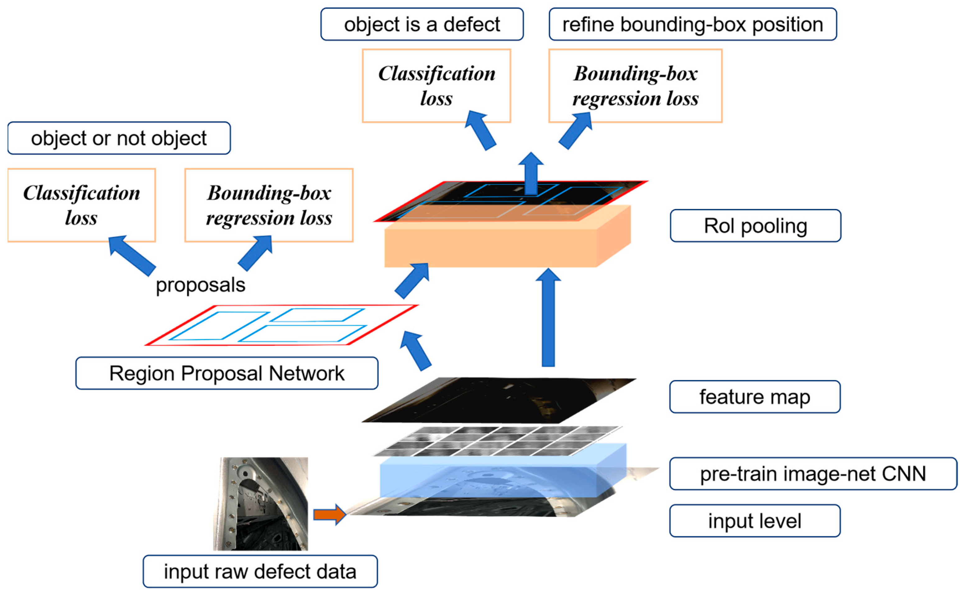
The Faster R-CNN detection algorithm can be divided into three main parts: convolution feature sharing, RPN candidate region decision-making, target regression, and classification calculation. Its overall structure is shown in Figure 1.
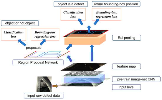
Figure 1.
Overall structure of the Faster R-CNN detection algorithm.
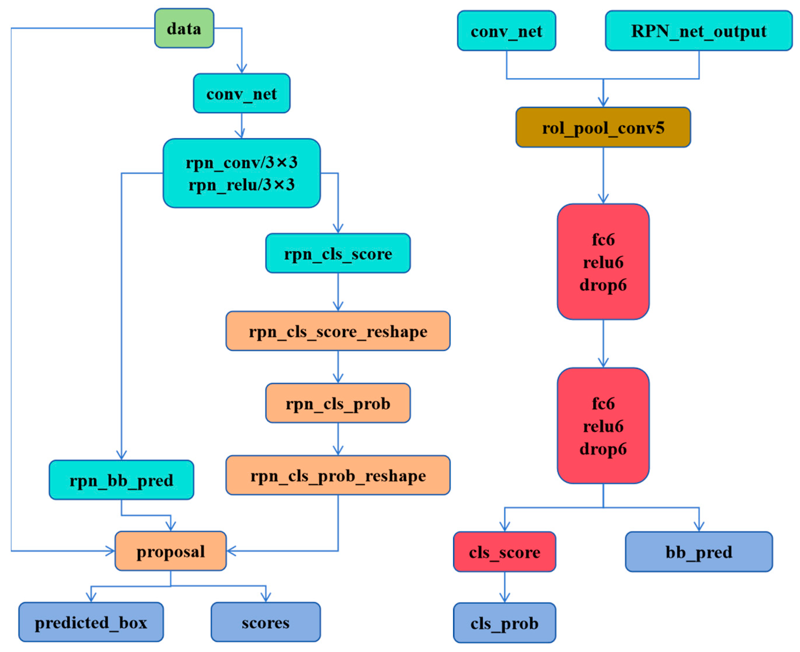
The network is further split into two sub-networks, each responsible for detecting defects and confirming defects, respectively. The RPN network is responsible for detecting whether there are defects, and the Fast RCNN network confirms the detailed information of the defects. The test network structure of the two sub-models is shown in Figure 2.
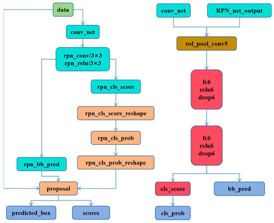
Figure 2.
Improved training network structure diagram. The RPN_forward structure (left), the Fast R-CNN structure (right).
The feature extraction layer architecture of the Faster R-CNN algorithm is similar to other convolutional neural networks. It is a combination of a series of convolutional layers, pooling layers, and ReLU activation layers. In the algorithm, the author performs feature extraction operations based on the two structures of VGG-16 and ZF, respectively. The comparison between the two is shown in Table 2.
Table 2.
Comparison of feature extraction layer structure based on VGG-16 and ZF.
From the comparison of the above table, we can see that VGG-16 has more layers and a deeper network, so it is conducive to extracting more subtle features. However, the huge number of parameters affect the calculation speed. Compared with ZF, the detection speed is greatly improved, and at the same time, it can guarantee a higher accuracy rate (62.1%). Therefore, the feature extraction layer based on the ZF structure is used in this article to satisfy real-time requirements for welding spot defect detection.
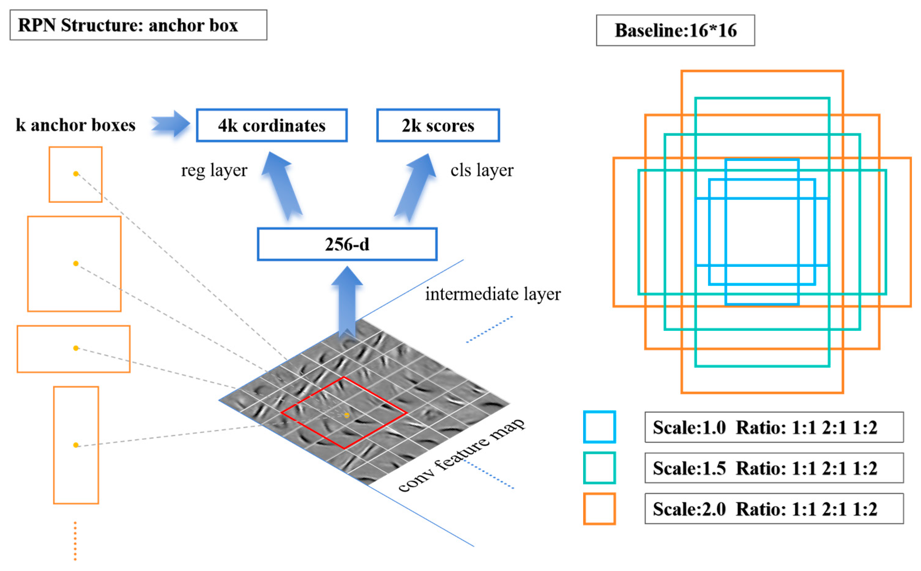
The feature map, generated after extraction by the convolutional network, is input to the RPN network to generate a series of rectangular region candidate frames and scores. Different from the manual sliding window target area selection method based on the SS algorithm, RPN uses a neural network to further extract the feature map features and generate anchor boxes of different scales (the number is k) at each point of the feature map. These anchor boxes are mapped to the original image, where coordinate regression calculation and target judgment are carried out through the neural network. At each feature point, RPN predicts 2k scores (probability of being/not the target) and 4k values (target coordinates). The detailed RPN structure is shown in Figure 3.
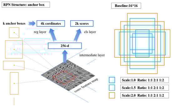
Figure 3.
RPN structure (left); anchor box setting diagram (right).
2.2. Optimizations on Anchor Box, RPN Box Selection, and Training Loss
In order to adapt to different detection sizes, the anchor can change the size according to the actual detection situation and adjust the ratio of width to height and zoom ratio. The size of the receptive field of the feature map is the basic size of the anchor setting. In the ZF model, after multi-convolutional layer down-sampling, the receptive field of the feature map is 16 × 16. Therefore, the anchors can be adjusted by stretching or zooming based on this 16 × 16 measurement. The size of the defect image detected in this article is 640 × 480. After the feature extraction of the convolutional layer, the feature map size is 50 × 37, then a total of 50 × 37 × k anchor boxes are generated, and k is the number of anchor box types. The anchor box setting diagram is shown in Figure 3.
During the training process, each anchor box may be close to the ground truth box (the target marked in the training sample). We need to judge whether the anchor has a target based on the relationship between the anchor box and the adjacent ground truth box, so we adopt the method of calculating the intersection-over-union ratio IoU, as shown in Equation (1). The IoU measures the closeness between the anchor box and the ground truth box by the ratio of the overlapping area to the total area.
The anchor is marked according to the value of IoU to determine whether the anchor participates in training. The marking method is expressed in Equation (2).
It can be seen from the above that an anchor box corresponding to the same ground-truth box is considered a positive sample if the IoU is the maximum value or the value is greater than 0.7 and a negative sample if the value is less than 0.3; the rest are excluded from the training after preliminary marking and screening. This greatly reduces the number of anchor box training and only trains the samples that have an impact on the result. Random sampling is performed in batches in the marked anchor box samples during the training process and each batch of data ensures that the data from the positive sample and the data from the negative sample are 1:1.
In the RPN model, the confidence of the b-box prediction the probabilities of being an object or belonging to the background, which is predicted by a two-class Softmax layer. During the forward pass of the network, we can select top N predictions with a higher score (probability) for being an object for the downstream defect category identification and box refinement. In the Region Proposal Network (RPN) used in Faster R-CNN, anchor box confidence scores are calculated to indicate the likelihood that a given anchor contains an object.
For each prediction box, we need to perform category output and coordinate regression output. The category output can use the Softmax function to calculate the probability of belonging to the positive sample and the negative sample, respectively. The coordinate regression output uses the feed-forward operation to obtain the coordinates of the prediction box and calculate the offset between the prediction box and the anchor box and the offset between the ground-truth box and the anchor box to minimize the difference between the two offsets. The offset between the two coordinates can be expressed as Equation (3):
: the center coordinates, width, and height of the anchor box;
: the center coordinates, width, and height of the ground truth box.
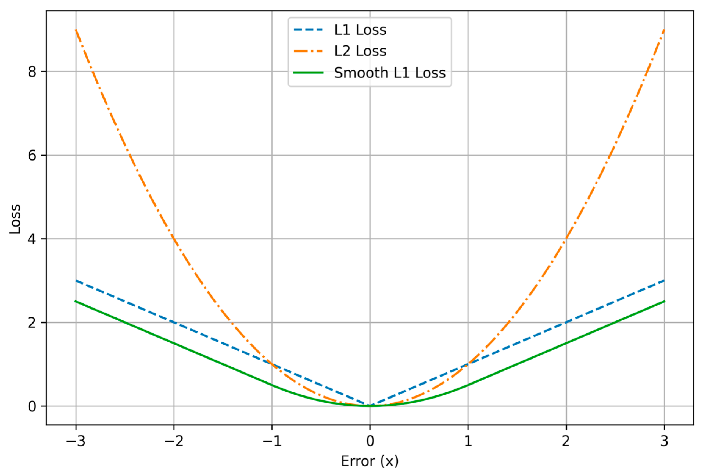
During training, a joint optimization method of multi-task solving is adopted, with the loss function comprising classification loss and regression loss. In this article, the positive and negative samples of the anchor box are marked as a multi-class problem, using the Softmax output unit and a loss function based on a negative algorithm. For the coordinate prediction of the anchor box, which is a regression problem, the improved SmoothL1 loss function is used to calculate the distance between the predicted coordinates and the true value. The loss function is expressed in Equation (4):
Fast R-CNN target detection calculation includes two stages. First, the selected candidate frame is matched with the feature map extracted by the convolutional layer. Next, the feature map is pooled with a fixed size so that the feature map dimensions are consistent when entering the fully connected layer. At the end of the network, the Softmax output unit is also used to determine the specific types of defects and the Smooth loss function is used to correct the position of the defect to output more accurate position coordinates.
The optimization of the bounding box prediction is a regression problem, which can be formulated as follows: Given an input image , where H, W, and C are the height, width, and number of channels of the image, a neural network is used to predict a set of continuous coordinates . The network function can be represented as follows:
where denotes the parameters (weights and biases) of the neural network. For a dataset with samples, the goal is to minimize the prediction error between the true coordinates . The typical loss function for this regression task can be loss, loss, and the Smooth loss function used in this paper.
where is the true coordinate vector, is the predicted coordinate vector, and is the total number of samples. The objective is to find the parameters that minimize the loss function:
As shown in Equations (5)–(7) and Figure 4, we can find that loss has a constant gradient to the prediction error. When the error approaches 0, the constant gradients could make the network optimization hard to converge to the ground truth. In contrast, ’s gradient is proportional to the prediction error. When the prediction error becomes smaller, the gradient approaches 0, which offers the network stability to converge to the ground truth. However, when the error is too large, especially at the beginning of the training, the large gradients could also cause instabilities. Smooth loss reaches a trade-off between and . It has a constant gradient when the error is large and a small gradient when the error is small. It has shown better robustness in many other bounding box regression problems [35].
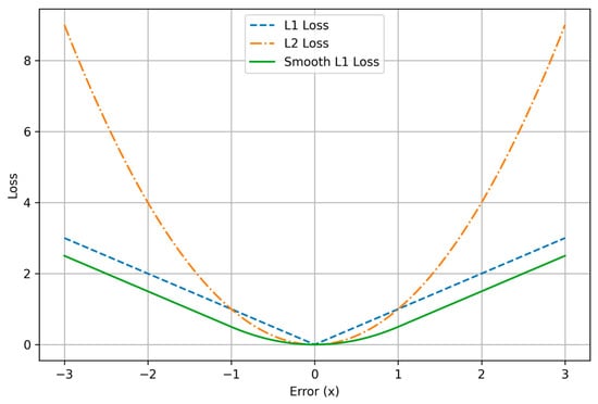
Figure 4.
Comparison of , , and Smooth losses.
This article focuses on the common defects in actual production. According to statistics of existing defect samples, it is found that the largest defect is about pixels, and the smallest defect is about pixels. Therefore, the initial setting is 12 kinds of anchor boxes . The ratio of width to height is [0.5,1,2] to cover the shape and size of the actual defect as much as possible. At this time, k = 12. When setting the convolution kernel dimension of RPN classification and regression output, it is also modified to cls: 2k = 24, reg: 4k = 48.
2.3. Neural Network Pruning
Neural network parameters are numerous and require a lot of computing resources and memory, which makes it very difficult to deploy neural networks in the embedded devices industry. Therefore, we propose to prune the original Faster R-CNN architecture using structure pruning, aiming to search for an architecture that can achieve the best tradeoff between performance and efficiency. We iteratively remove the parameters of the model. For each t, we then conduct layer-wise pruning by removing a complete layer if the pruned model can achieve better performance after fine-tuning. We summarize this procedure as an algorithm in Algorithm 1.
| Algorithm 1 Structured Pruning of Faster RCNN model |
| 1: Input: Pretrained CNN model M, pruning thresholds {1/8, 1/4, 1/2}, layers {L1, L2, …, Ln} Excluding first and last layers 2: Output: Pruning configuration and Pruned model M’ 3: Initialize pruned model M’ ← M 4: for each threshold do 5: Remove portion of parameters in M’ 6: Fine-tune M’ on training data 7: Evaluate performance of M’ 8: for each layer do 9: Temporarily remove layer Li from M’ 10: Fine-tune M’ on training data 11: Evaluate performance of M’ 12: if Performance improves then 13: Permanently remove layer Li from M’ 14: else 15: Restore layer Li in M’ 16: end if 17: end for 18: Save the pruning configuration and the pruned model of the best performance 19: end for 20: Take the best model from as M’ 21: Return Pruned model M’ |
3. Experiments and Discussions
3.1. Dataset and Evaluation Metric
3.1.1. Dataset Preparation
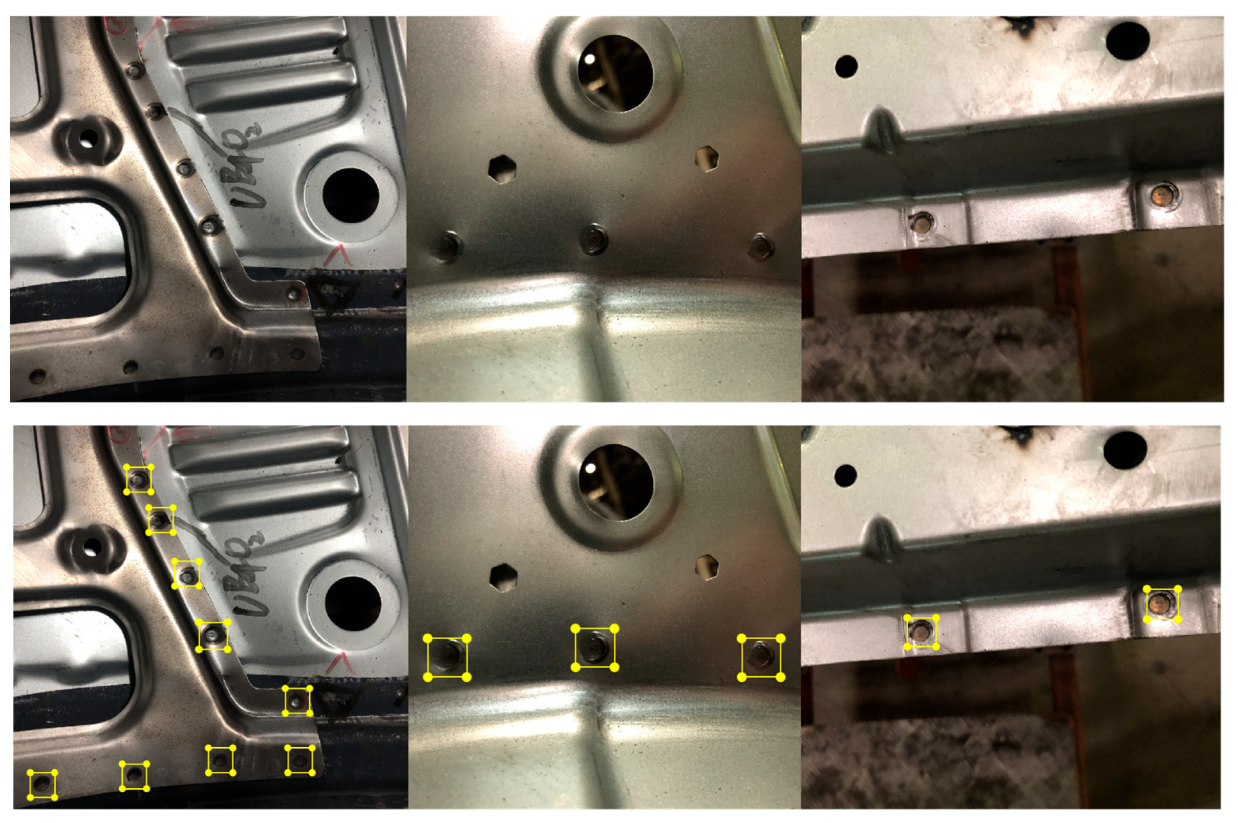
For the algorithm validation, the object detection model requires a well-labeled dataset. As no pre-existing dataset for auto body spot welds is available, 1000 images of spot welds at various positions were collected from an automotive assembly line. The RSW quality vision inspection experimental platform is depicted in Figure 5. By varying the position of the robot arm, numerous welding images were captured using an RGB camera, Intel RealSense d435 (Shanghai, China). Each image in the dataset has a resolution of 4032 × 3024 pixels, with some spot welds representing only one-thousandth of the total image, making them small targets. The spot welds were annotated to form a body welding spot detection dataset consisting of 800 images for training and 200 for testing.
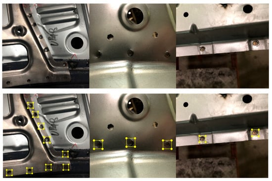
Figure 5.
Image samples of body-in-white welding spots and labels.
The imbalance of the data means the imbalanced ratio between the normal spot and the abnormal spot. In practice, the frequency of the abnormal data is below 0.1%, i.e., every 1000 welding contains no more than one abnormal spot on average. The dataset used in this article is collected from the industrial partner in the real-world production line, containing approximately 10% abnormal spots. To alleviate the data imbalance problem, we apply data augmentation techniques to increase the data quantity and diversity.
An expert engineer annotated the spot welds and classified their quality as “normal” or “abnormal”, which served as the ground truth. The defective welding spots were further categorized by defect type, such as overlaps, edge welds, cold welds, etc. Samples of BIW welding spots and labels are displayed in Figure 5.
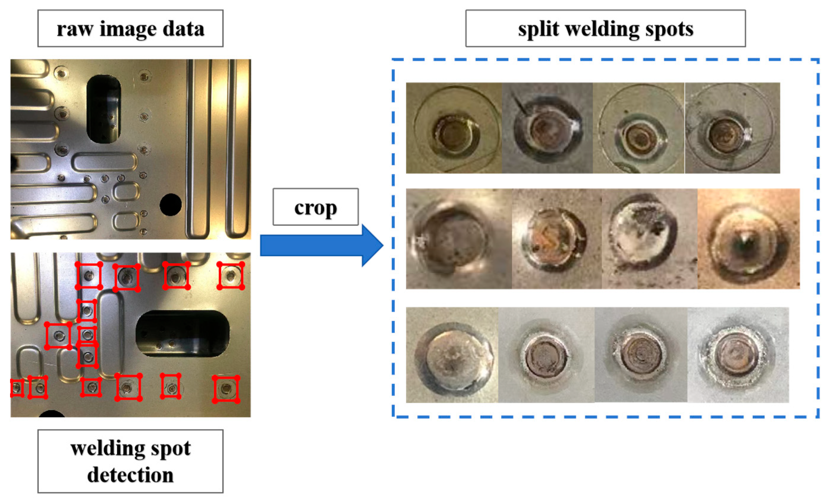
Figure 6 further illustrates the process of welding spot image acquisition and localization. The left side shows an image of a welding plate with multiple welding spots highlighted by red boxes, indicating that the system has successfully located and identified the welding areas on the plate. These highlighted regions are then cropped and displayed within the dashed frame on the right. Each welding spot exhibits different quality characteristics, potentially including both normal and defective spots. This process involves segmenting the welding spot images and categorizing them, ultimately facilitating quality inspection.
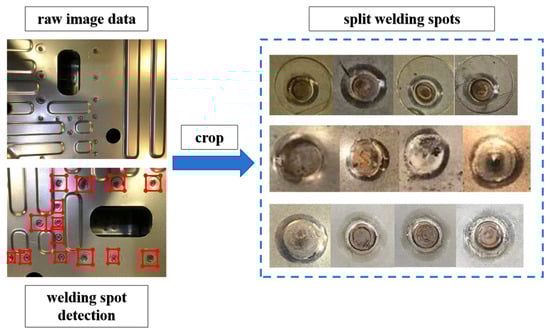
Figure 6.
The procedure diagram of the welding spot quality inspection process.
The experiments were performed on a system equipped with an NVIDIA 2080ti GPU (NVIDIA, Shanghai, China), using the PyTorch v2.5 deep learning framework for implementation. The input images used for training were resized to 256 × 256 pixels resolution. A total of 1035 images were employed for model training processing and data augmentation. By using the Adam optimization method [36], we set 500 epochs in the training stage, with a learning rate of 0.02 and a batch size of eight. We compare our proposed model with some typical surface detection models, such as SSD and CNN-Lenet5 [37].
3.1.2. Evaluation Metrics
In this work, mAP (mean Average Precision) is used to evaluate the overall accuracy of object detection by considering both precision and recall across all classes. Recall measures the model’s ability to detect all true positive instances, highlighting its sensitivity. The F1-score represents the harmonic mean of precision and recall, providing a balanced evaluation of detection performance. FPS (Frames Per Second) assesses the inference speed of the model, indicating its real-time processing capability. Together, these metrics comprehensively evaluate the effectiveness and efficiency of the proposed approach.
3.2. Experimental Results and Discussions
3.2.1. Comparison Between the Proposed Model and Typical Model
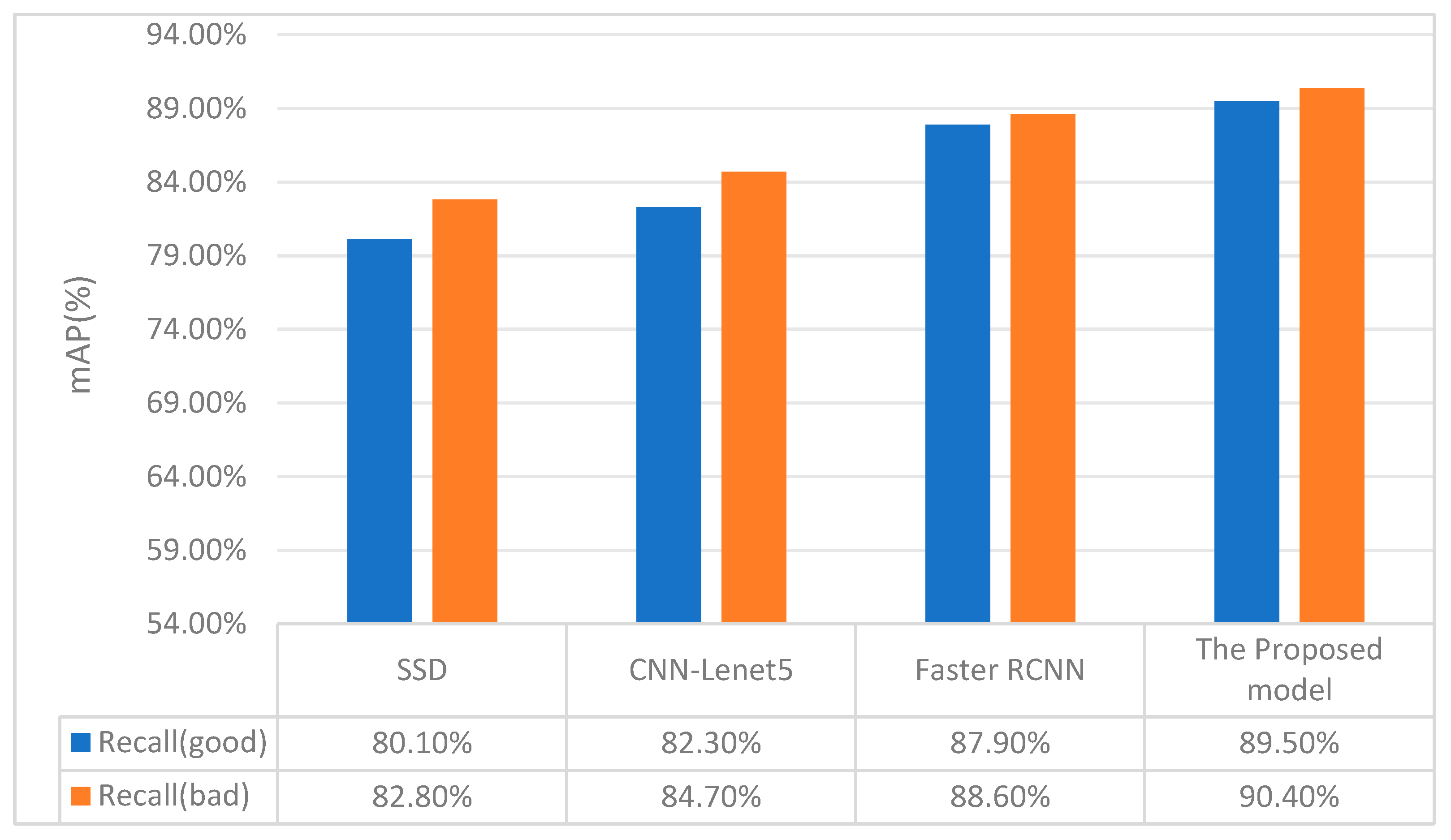
A comparison between SSD, CNN-Lenet5, classical Faster RCNN, and the proposed model is conducted by visualizing images in Table 3 and Figure 7. Table 4 shows the mean Average Precision (mAP) and the speed of each model. Figure 7 shows the recall rate of normal and abnormal samples relatively. Compared to the other models, the proposed approach significantly improves accuracy, even with a slight increase in time.
Table 3.
Comparison between the proposed model and typical models.
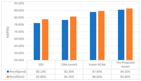
Figure 7.
The comparison of recall rates of different models.
Table 4.
Model pruning optimization experiment.
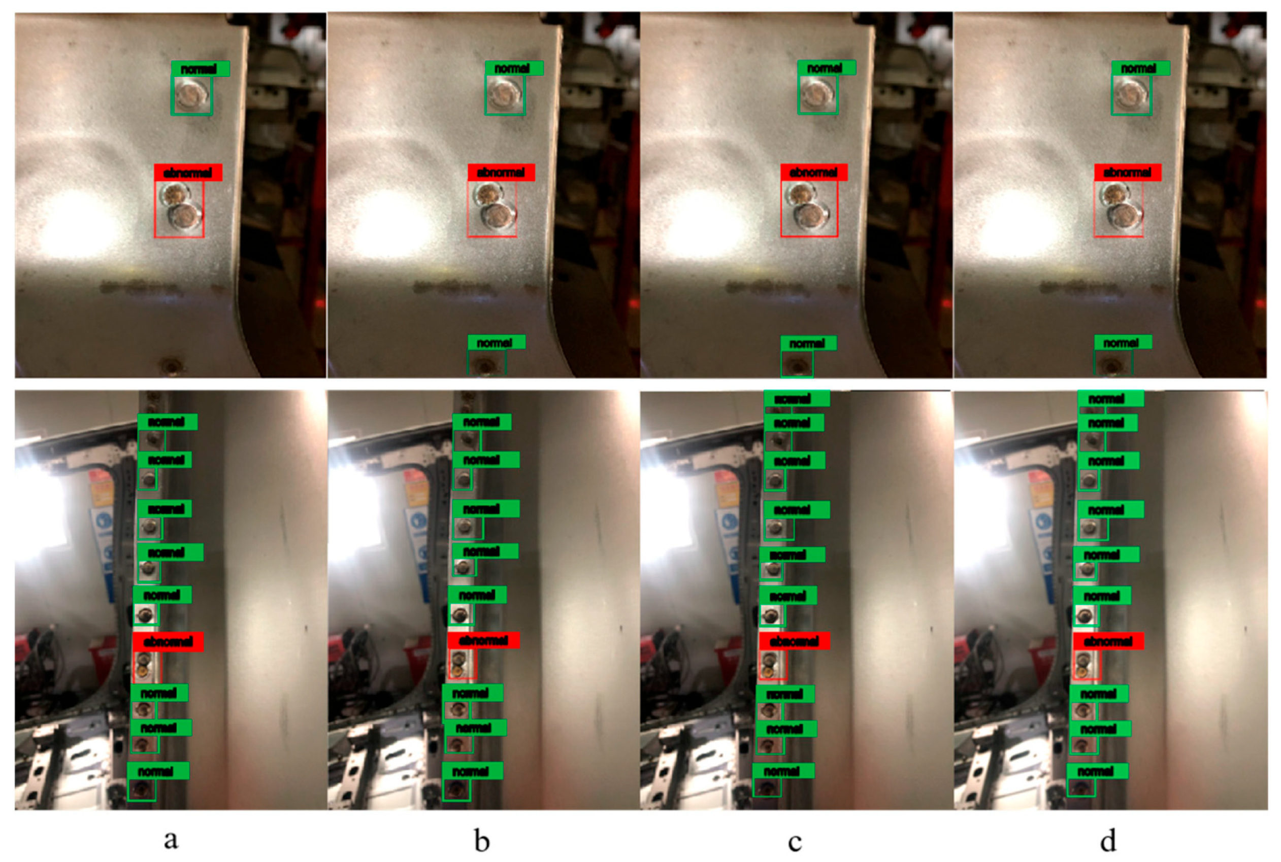
Figure 8 shows the results of several samples to show the performance of different models: SSD model (a), CNN-Lenet5 (b), Faster RCNN (c), and the proposed model (d). The green boxes denote the good welding spots, while the red ones indicate the bad samples. It can be found that the proposed model can recognize the good and bad welding spots well. To further validate the model’s prediction and generalization ability, some objects in the training set were artificially unlabeled. Results demonstrate that it successfully identified the previously missed spot welds, as demonstrated in Figure 8, confirming the good performance of the proposed model.
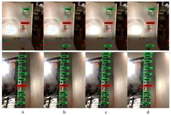
Figure 8.
The results of several samples to show the performance of different models. SSD model (a), CNN-Lenet5 (b), Faster RCNN (c), and the proposed model (d).
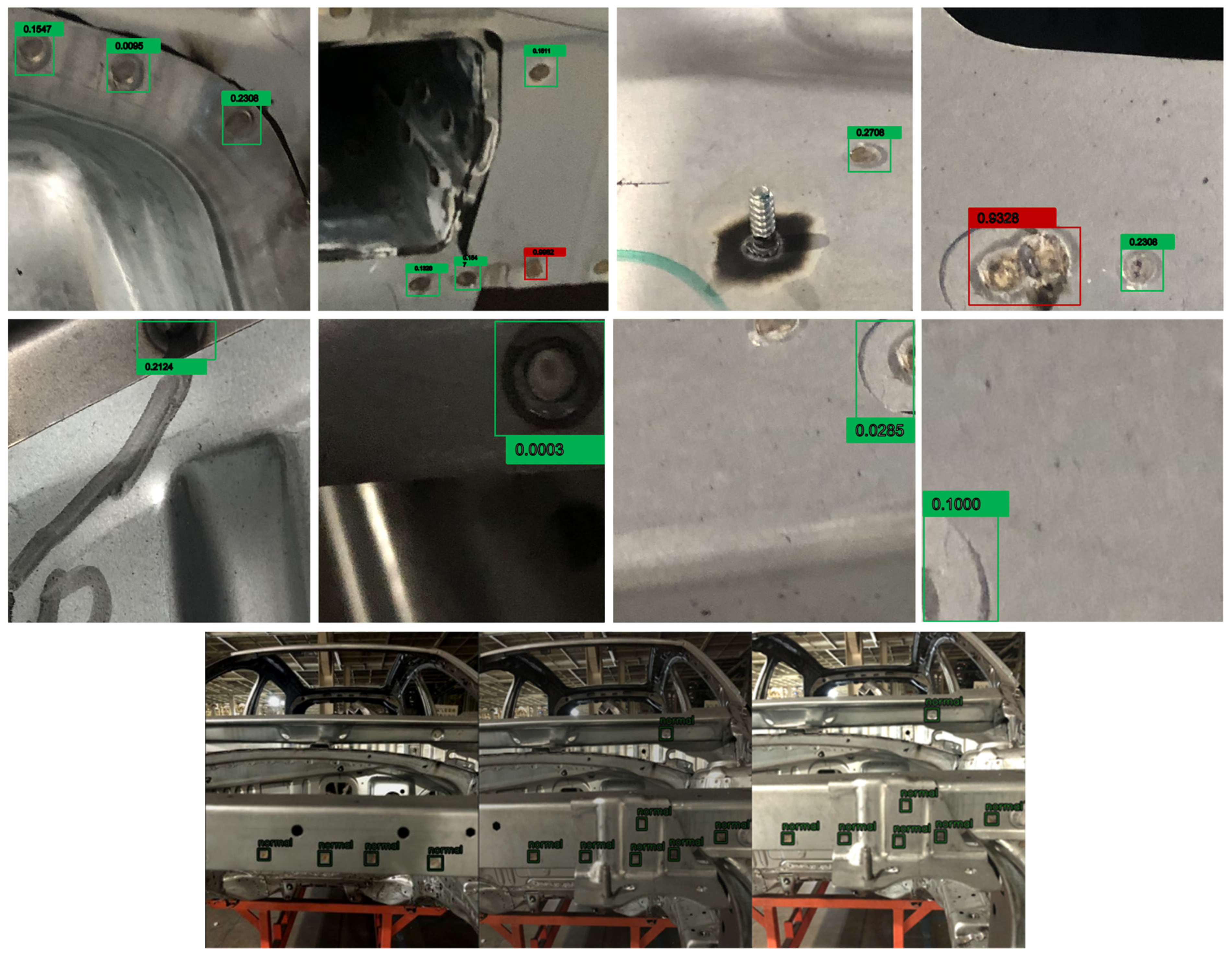
Figure 9 shows some additional examples of detected defects in the testing data. To verify the detection performance and generalization capability of the proposed model, we conducted tests using both cropped images and original images. Additional examples demonstrate that the proposed model achieves a high level of detection accuracy in real production environments and exhibits strong generalization capability. The defect positive and negative sample labels are normalized between (0, 1). A result closer to 0 indicates a higher probability of a normal weld, whereas a value closer to 1 suggests a defective weld.
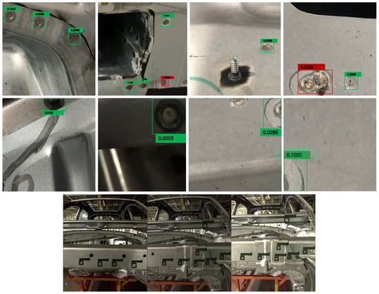
Figure 9.
Additional examples of detected defects on the testing data.
3.2.2. Study of Neural Network Pruning
In this section, we propose a pruning algorithm in order to reduce the redundant parameters of the model, improve the detection speed, and facilitate the deployment of the neural network model in the actual production detection system. In this paper, combined with the visualization results of the output of each layer, pruning experiments on different scales of the model are carried out, and the structure and parameters of the model are optimized. The experiment content is shown in Table 4.
Analysis of pruning optimization experiment results:
It can be seen from experiments 1–4 that with the decrease in network parameters, the training time and testing time both decrease significantly. From the test results, the reduction in parameters will cause the fluctuation of test mAP (mean Average Precision). According to the analysis, there are two reasons for this phenomenon: one is that modifying the entire network prevents migration learning based on the pre-trained model, resulting in insufficient model training; the other is that modifying the model to a large extent damages the model’s detection capability. However, in general, the modified models of different scales all have better detection performance, which shows that the algorithm has a certain degree of stability and robustness.
It can be seen from experiments 1, 6, and 7 that the fully connected layer occupies most of the parameters of the entire network, and the pruning of the fully connected layer has an obvious effect on reducing the number of parameters of the entire model. After pruning the fully connected layer, the model checking performance has improved significantly (mAP: 91.2%). Experiment 7 is carried out on the basis of Experiment 5 and Experiment 6, and the fourth convolutional layer and the fully connected layer are pruned at the same time.
The experimental results show that the model parameters are reduced by about 50%, the amount of calculation is reduced, and the training of the model is greatly reduced. Detection time and model detection performance have been further improved (mAP: 92.5%). The reason for the improved performance after analysis is that because the training data set used by the model in this article is small and the data distribution is simple, it is easy to train with a more complex model. The phenomenon of over-fitting is caused by the targeted reduction in network parameters, which reduces the non-linearity of the network, reduces the occurrence of over-fitting to a certain extent, and improves the detection performance of the model.
4. Conclusions
- (1)
- scientific contribution
This paper aims to predict the welding spot defects during the production of body-in-white by constructing an inspection system using an improved, faster R-CNN model. This deep learning network model shows good performance on surface quality inspection for small object detection. This paper makes the following scientific contributions to the field of resistance welding spot defect detection:
Enhanced Localization Mechanism: The study improves the Faster R-CNN model by refining the selection of anchor boxes in the RPN network, utilizing high-confidence anchor boxes to localize welding spots more accurately. This innovation significantly enhances the accuracy and efficiency of defect detection systems for small object detection.
Lightweight Pruning Model Design: A novel pruning approach is proposed to optimize the backbone network by removing redundant convolutional and connection layers, as well as reducing unnecessary parameters in hidden layers. This design reduces the computational cost, speeds up the processing time, and maintains high detection accuracy.
Real-Time Detection Optimization: The proposed model achieves a testing speed of 15 ms per image, with detection accuracy and recall rates exceeding 90%. This optimization fulfills industrial requirements for both efficiency and precision in real-time welding spot quality inspection.
Practical Applicability for Body-in-White Production: By addressing the specific challenges of welding spot defect detection in body-in-white manufacturing, the research provides an efficient and accurate inspection system that meets industrial standards, making it highly applicable for real-world deployment.
These contributions demonstrate a significant step toward integrating deep learning-based inspection methods into industrial production lines, advancing the state-of-the-art quality control for resistance welding.
- (2)
- Novelty
This approach improves the Faster R-CNN model by refining the anchor box selection in the RPN network. The method selects anchor boxes with higher confidence levels for weld spot localization, thereby improving both the accuracy and efficiency of the detection system.
A novel pruning model is introduced, removing redundant convolutional and connection layers within the backbone network and reducing some parameters in each hidden layer. This design significantly decreases the model’s parameter count and improves detection speed while maintaining detection accuracy.
The proposed model achieves a testing speed of 15 ms per image, with detection accuracy and recall rates both exceeding 90%, meeting the high efficiency and precision requirements of welding spot defect detection.
- (3)
- Limitation
Due to the actual environment of the production line, we are unable to collect sufficient data samples. The number of samples in the dataset is insufficient and unbalanced when the model is trained, which may cause over-fitting, leading to missed detection and recognition errors in the real test.
The predicted welding spot defects in question here are particularly surface welding spot defects and not welding spot defects in general. Therefore, The detection performance is also limited due to the fact that the volume spot welding defects can apparently go undetected here.
- (4)
- Future work
The abundance of data plays a vital role in the performance of deep learning algorithms. In future work, it is necessary to improve the data management system, increase the number of samples, and improve the quality of samples. We hope to make some progress in the aspect of novel data augmentation.
Faster R-CNN, while accurate, is still slower than models such as YOLO or SSD when used in real-time production environments. Future developments could focus on optimizing the Region Proposal Network (RPN) or incorporating lightweight architectures such as MobileNet or EfficientNet into the Faster R-CNN pipeline to reduce inference time while maintaining accuracy.
Surface defects in weld spots often vary in size, from small cracks to large spatters. Faster R-CNN already handles multi-scale detection to some degree, but enhancing this capability, potentially through multi-scale feature extraction techniques such as Feature Pyramid Networks (FPN), could lead to even better detection of tiny or barely visible defects.
Future research should also focus on integrating multiple validation techniques, including metallographic analysis, destructive testing, ultrasonic inspection, X-ray imaging, and statistical comparison, to establish a comprehensive and systematic evaluation framework for weld defect detection. By combining the strengths of each method, such as the precision of metallography, the performance insights from destructive testing, and the scalability of non-destructive methods such as ultrasonic and X-ray inspections, researchers can improve the reliability and applicability of visual inspection models. Furthermore, statistical analysis can help refine defect classification thresholds and enhance the accuracy of predictive models, paving the way for more robust and automated welding quality control systems.
Author Contributions
Conceptualization, W.L. and J.H.; methodology, W.L.; data collection, W.L., J.Q. and J.H.; writing—original draft preparation, W.L.; writing—review and editing, J.Q.; supervision, W.L.; validation, W.L.; funding acquisition, J.H. All authors have read and agreed to the published version of the manuscript.
Funding
This research is supported by the National Natural Science Foundation of China (U23B20102, 52035007), Ministry of Education “Human Factors and Ergonomics” University Industry Collaborative Education Project (No. 202209LH16).
Data Availability Statement
For the private RSW in BIW datasets, requests for access can be directed to weijie.liu@sjtu.edu.cn.
Acknowledgments
We would like to thank Hongpeng Cao for his insightful discussion and feedback on technical details.
Conflicts of Interest
The authors declare that they have no known competing financial interests or personal relationships that could have appeared to influence the work reported in this paper. The authors declare no conflicts of interest. The funders had no role in the design of the study; in the collection, analyses, or interpretation of data; in the writing of the manuscript; or in the decision to publish the results.
References
- Zhou, K.; Yao, P. Overview of recent advances of process analysis and quality control in resistance spot welding. Mech. Syst. Signal Process. 2019, 124, 170–198. [Google Scholar] [CrossRef]
- Wang, J.; Zhang, Z.; Bai, Z.; Zhang, S.; Qin, R.; Huang, J.; Wen, G. On-line defect recognition of MIG lap welding for stainless steel sheet based on weld image and CMT voltage: Feature fusion and attention weights visualization. J. Manuf. Process. 2023, 108, 430–444. [Google Scholar] [CrossRef]
- Hong, Y.; He, X.; Xu, J.; Yuan, R.; Lin, K.; Chang, B.; Du, D. AF-FTTSnet: An end-to-end two-stream convolutional neural network for online quality monitoring of robotic welding. J. Manuf. Syst. 2024, 74, 422–434. [Google Scholar] [CrossRef]
- Dai, W.; Li, D.; Tang, D.; Jiang, Q.; Wang, D.; Wang, H.; Peng, Y. Deep learning assisted vision inspection of resistance spot welds. J. Manuf. Process. 2021, 62, 262–274. [Google Scholar] [CrossRef]
- Honarvar, F.; Varvani-Farahani, A. A review of ultrasonic testing applications in additive manufacturing: Defect evaluation, material characterization, and process control. Ultrasonics 2020, 108, 106227. [Google Scholar] [CrossRef] [PubMed]
- Mirmahdi, E.; Afshari, D.; Ivanaki, M.K. A Review of Ultrasonic Testing Applications in Spot Welding: Defect Evaluation in Experimental and Simulation Results. Trans. Indian Inst. Met. 2023, 76, 1381–1392. Available online: https://link.springer.com/article/10.1007/s12666-022-02738-8 (accessed on 17 October 2024). [CrossRef]
- Yang, L.; Chuai, R.; Cai, G.; Xue, D.; Li, J.; Liu, K.; Liu, C. Ultrasonic Non-Destructive Testing and Evaluation of Stainless-Steel Resistance Spot Welding Based on Spiral C-Scan Technique. Sensors 2024, 24, 4771. Available online: https://www.mdpi.com/1424-8220/24/15/4771 (accessed on 17 October 2024). [CrossRef]
- Posilovic, L. Generative Adversarial Networks for Ultrasound Image Synthesis and Analysis in Nondestructive Evaluation. Ph.D. Thesis, University of Zagreb, Zagreb, Croatia, 2022. [Google Scholar]
- Juengert, A.; Werz, M.; Gr. Maev, R.; Brauns, M.; Labud, P. Nondestructive Testing of Welds. In Handbook of Nondestructive Evaluation 4.0; Springer: Berlin/Heidelberg, Germany, 2022; Available online: https://link.springer.com/referenceworkentry/10.1007/978-3-030-73206-6_2 (accessed on 17 October 2024).
- Maeda, K.; Suzuki, R.; Suga, T.; Kawahito, Y. Investigating Delayed Cracking Behaviour in Laser Welds of High Strength Steel Sheets Using an X-ray Transmission In-Situ Observation System. Sci. Technol. Weld. Join. 2020, 25, 377–382. Available online: https://www.tandfonline.com/doi/abs/10.1080/13621718.2020.1714873 (accessed on 17 October 2024). [CrossRef]
- Butsykin, S.; Gordynets, A.; Kiselev, A.; Slobodyan, M. Evaluation of the Reliability of Resistance Spot Welding Control via on-Line Monitoring of Dynamic Resistance. J. Intell. Manuf. 2023, 34, 3109–3129. Available online: https://link.springer.com/article/10.1007/s10845-022-01987-0 (accessed on 17 October 2024). [CrossRef]
- Wang, L.; Hou, Y.; Zhang, H.; Zhao, J.; Xi, T.; Qi, X.; Li, Y. A New Measurement Method for the Dynamic Resistance Signal During the Resistance Spot Welding Process. Meas. Sci. Technol. 2016, 27, 095009. Available online: https://iopscience.iop.org/article/10.1088/0957-0233/27/9/095009/meta (accessed on 17 October 2024). [CrossRef]
- Safari, M.; Mostaan, H.; Yadegari Kh, H.; Asgari, D. Effects of Process Parameters on Tensile-Shear Strength and Failure Mode of Resistance Spot Welds of AISI 201 Stainless Steel. Int. J. Adv. Manuf. Technol. 2017, 89, 1853–1863. Available online: https://link.springer.com/article/10.1007/s00170-016-9222-z (accessed on 17 October 2024). [CrossRef]
- Radakovic, D.J.; Tumuluru, M. Predicting Resistance Spot Weld Failure Modes in Shear Tension Tests of Advanced High-Strength Automotive Steels. Available online: https://citeseerx.ist.psu.edu/document?repid=rep1&type=pdf&doi=dc0e4de080d7199c22fc171b82c61cea04f0d5da (accessed on 17 October 2024).
- Tsukada, K.; Miyake, K.; Harada, D.; Sakai, K.; Kiwa, T. Magnetic Nondestructive Test for Resistance Spot Welds Using Magnetic Flux Penetration and Eddy Current Methods. J. Nondestruct. Eval. 2013, 32, 286–293. Available online: https://link.springer.com/article/10.1007/s10921-013-0181-0 (accessed on 17 October 2024). [CrossRef]
- Dahmene, F.; Yaacoubi, S.; Mountassir, M.E.; Bouzenad, A.E.; Rabaey, P.; Masmoudi, M.; Nennig, P.; Dupuy, T.; Benlatreche, Y.; Taram, A. On the Nondestructive Testing and Monitoring of Cracks in Resistance Spot Welds: Recent Gained Experience. Weld. World 2022, 66, 629–641. Available online: https://link.springer.com/article/10.1007/s40194-022-01249-w (accessed on 17 October 2024). [CrossRef]
- Sak, H.; Senior, A.; Rao, K.; Beaufays, F. Fast and Accurate Recurrent Neural Network Acoustic Models for Speech Recognition. 2015. Available online: https://www.isca-archive.org/interspeech_2015/sak15_interspeech.pdf (accessed on 17 October 2024).
- Ye, S.; Guo, Z.; Zheng, P.; Wang, L.; Lin, C. A Vision Inspection System for the Defects of Resistance Spot Welding Based on Neural Network. In Computer Vision Systems; Springer: Berlin/Heidelberg, Germany, 2017; Available online: https://link.springer.com/chapter/10.1007/978-3-319-68345-4_14 (accessed on 17 October 2024).
- Yang, Y.; Zheng, P.; He, H.; Zheng, T.; Wang, L.; He, S. An Evaluation Method of Acceptable and Failed Spot Welding Products Based on Image Classification with Transfer Learning Technique. In Proceedings of the Proceedings of the 2nd International Conference on Computer Science and Application Engineering, Hohhot, China, 22–24 October 2018; Association for Computing Machinery: New York, NY, USA, 2018; pp. 1–6. [Google Scholar]
- Jaderberg, M.; Simonyan, K.; Zisserman, A.; Kavukcuoglu, K. Spatial Transformer Networks. In Proceedings of the Advances in Neural Information Processing Systems, Montreal, QC, Canada, 7–12 December 2015; Curran Associates, Inc.: North Adams, MA, USA, 2015; Volume 28. Available online: https://proceedings.neurips.cc/paper_files/paper/2015/hash/33ceb07bf4eeb3da587e268d663aba1a-Abstract.html (accessed on 4 February 2016).
- Redmon, J.; Divvala, S.; Girshick, R.; Farhadi, A. You Only Look Once: Unified, Real-Time Object Detection. arXiv 2016, arXiv:1506.02640. [Google Scholar] [CrossRef]
- [1512.02325] SSD: Single Shot MultiBox Detector. Available online: https://arxiv.org/abs/1512.02325 (accessed on 17 October 2024).
- Lin, T.-Y.; Goyal, P.; Girshick, R.; He, K.; Dollár, P. Focal Loss for Dense Object Detection. arXiv 2018, arXiv:1708.02002. [Google Scholar] [CrossRef]
- Girshick, R.; Donahue, J.; Darrell, T.; Malik, J. Rich feature hierarchies for accurate object detection and semantic segmentation. arXiv 2014, arXiv:1311.2524. [Google Scholar] [CrossRef]
- He, K.; Zhang, X.; Ren, S.; Sun, J. Spatial Pyramid Pooling in Deep Convolutional Networks for Visual Recognition. In Computer Vision—ECCV 2014, Proceedings of the 13th European Conference, Zurich, Switzerland, 6–12 September 2014, Proceedings, Part III 13; Lecture Notes in Computer Science; Springer: Berlin/Heidelberg, Germany, 2014; Volume 8691, pp. 346–361. [Google Scholar]
- Girshick, R. Fast R-CNN. In Proceedings of the 2015 IEEE International Conference on Computer Vision (ICCV), Santiago, Chile, 7–13 December 2015; pp. 1440–1448. [Google Scholar]
- Ren, S.; He, K.; Girshick, R.; Sun, J. Faster R-CNN: Towards Real-Time Object Detection with Region Proposal Networks. arXiv 2016, arXiv:1506.01497. [Google Scholar] [CrossRef]
- Lin, T.-Y.; Dollár, P.; Girshick, R.; He, K.; Hariharan, B.; Belongie, S. Feature Pyramid Networks for Object Detection. In Proceedings of the 2017 IEEE Conference on Computer Vision and Pattern Recognition (CVPR), Honolulu, HI, USA, 21–26 July 2017; pp. 936–944. [Google Scholar]
- Cao, H.; Dirnberger, L.; Bernardini, D.; Piazza, C.; Caccamo, M. 6IMPOSE: Bridging the Reality Gap in 6D Pose Estimation for Robotic Grasping. arXiv 2023, arXiv:2208.14288. [Google Scholar] [CrossRef] [PubMed]
- Li, Y.; Huang, H.; Xie, Q.; Yao, L.; Chen, Q. Research on a Surface Defect Detection Algorithm Based on MobileNet-SSD. Appl. Sci. 2018, 8, 1678. Available online: https://www.researchgate.net/publication/327705107_Research_on_a_Surface_Defect_Detection_Algorithm_Based_on_MobileNet-SSD (accessed on 17 October 2024). [CrossRef]
- Wang, H.; Li, M.; Wan, Z. Rail surface defect detection based on improved Mask R-CNN. Comput. Electr. Eng. 2022, 102, 108269. [Google Scholar] [CrossRef]
- Luo, W.; Luo, J.; Yang, Z. FPC surface defect detection based on improved Faster R-CNN with decoupled RPN. In Proceedings of the 2020 Chinese Automation Congress (CAC), Shanghai, China, 6–8 November 2020; pp. 7035–7039. [Google Scholar]
- Oh, S.; Jung, M.; Lim, C.; Shin, S. Automatic Detection of Welding Defects Using Faster R-CNN. Appl. Sci. 2020, 10, 8629. [Google Scholar] [CrossRef]
- Simonyan, K.; Zisserman, A. Very Deep Convolutional Networks for Large-Scale Image Recognition. arXiv 2015, arXiv:1409.1556. [Google Scholar] [CrossRef]
- Gkioxari, G.; Girshick, R.; Malik, J. Contextual Action Recognition with R*CNN. arXiv 2016, arXiv:1505.01197. [Google Scholar] [CrossRef]
- Kingma, D.P.; Ba, J. Adam: A Method for Stochastic Optimization. arXiv 2017, arXiv:1412.6980. [Google Scholar] [CrossRef]
- Lecun, Y.; Bottou, L.; Bengio, Y.; Haffner, P. Gradient-based learning applied to document recognition. Proc. IEEE 1998, 86, 2278–2324. [Google Scholar] [CrossRef]
- He, K.; Zhang, X.; Ren, S.; Sun, J. Spatial Pyramid Pooling in Deep Convolutional Networks for Visual Recognition. IEEE Trans. Pattern Anal. Mach. Intell. 2015, 37, 1904–1916. Available online: https://ieeexplore.ieee.org/document/7005506 (accessed on 29 October 2024). [CrossRef]
- Li, C.; Li, L.; Jiang, H.; Weng, K.; Geng, Y.; Li, L.; Ke, Z.; Li, Q.; Cheng, M.; Nie, W.; et al. YOLOv6: A Single-Stage Object Detection Framework for Industrial Applications. arXiv 2022, arXiv:2209.02976. [Google Scholar] [CrossRef]
- Zhu, L.; Wang, X.; Ke, Z.; Zhang, W.; Lau, R. BiFormer: Vision Transformer with Bi-Level Routing Attention. arXiv 2023, arXiv:2303.08810. [Google Scholar] [CrossRef]
Disclaimer/Publisher’s Note: The statements, opinions and data contained in all publications are solely those of the individual author(s) and contributor(s) and not of MDPI and/or the editor(s). MDPI and/or the editor(s) disclaim responsibility for any injury to people or property resulting from any ideas, methods, instructions or products referred to in the content. |
© 2025 by the authors. Licensee MDPI, Basel, Switzerland. This article is an open access article distributed under the terms and conditions of the Creative Commons Attribution (CC BY) license (https://creativecommons.org/licenses/by/4.0/).