
Multi-Objective Optimization of Gear Design of E-Axles to Improve Noise Emission and Load Distribution


Abstract
:1. Introduction
- First step: macro-geometry optimization, based on an objective function that combines the contact ratio—closely related to sound pressure—with dissipated power and the center distance between shafts. To reduce the computational cost and explore a larger number of solutions, transmission error and, consequently, sound pressure are not computed at this stage. Only gear parameters are considered without shafts and their deflection.
- Second step: micro-geometry optimization, performed using sound pressure as the cost function, incorporating tooth contact analysis and transmission error calculation. Stress distribution is considered a constraint in the optimization process. Shafts, joints, and electric motors are considered with their structural behavior.
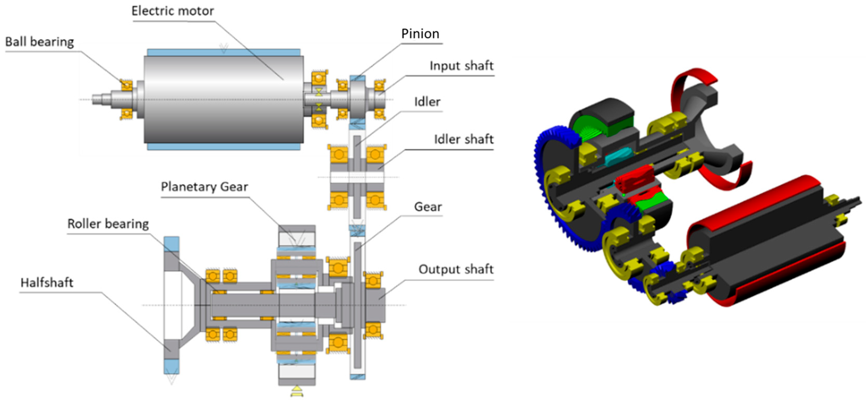
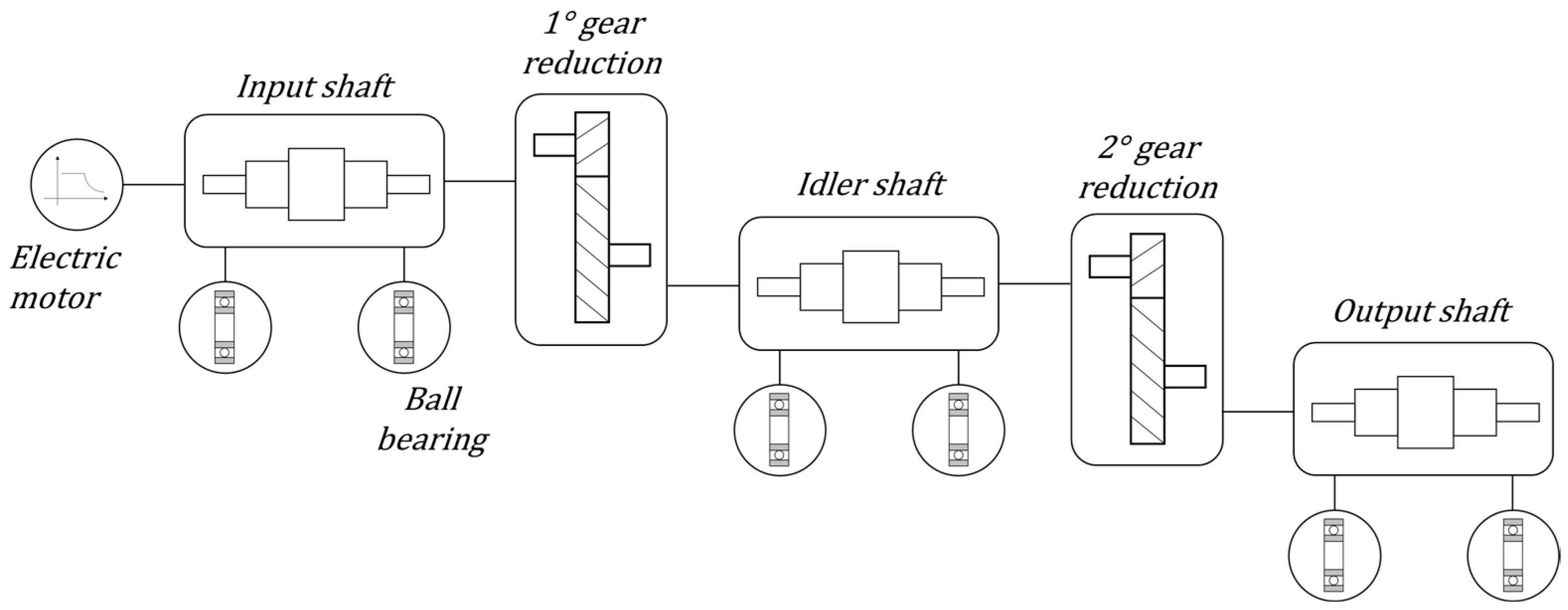
2. E-Axle Modeling Approach and Subcomponents
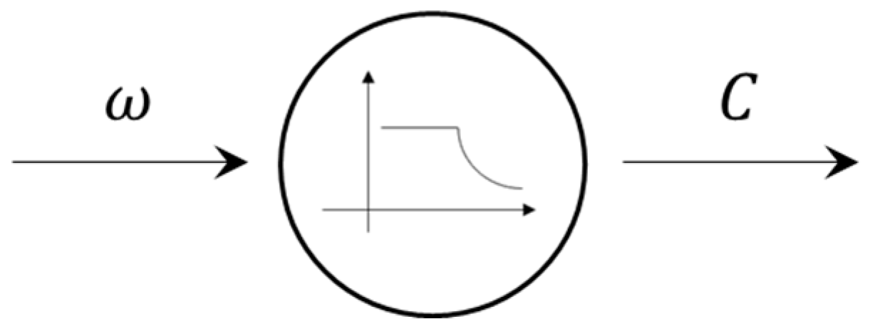
2.1. Electric Motor
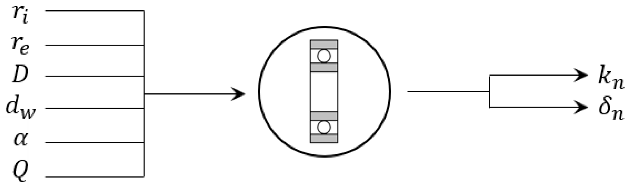
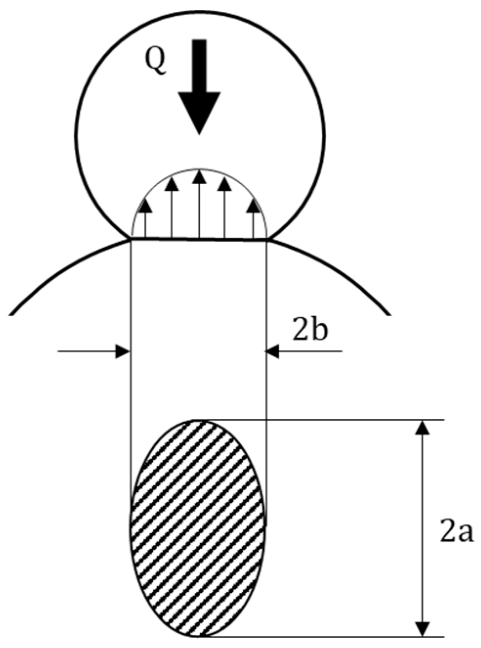
2.2. Ball Bearings
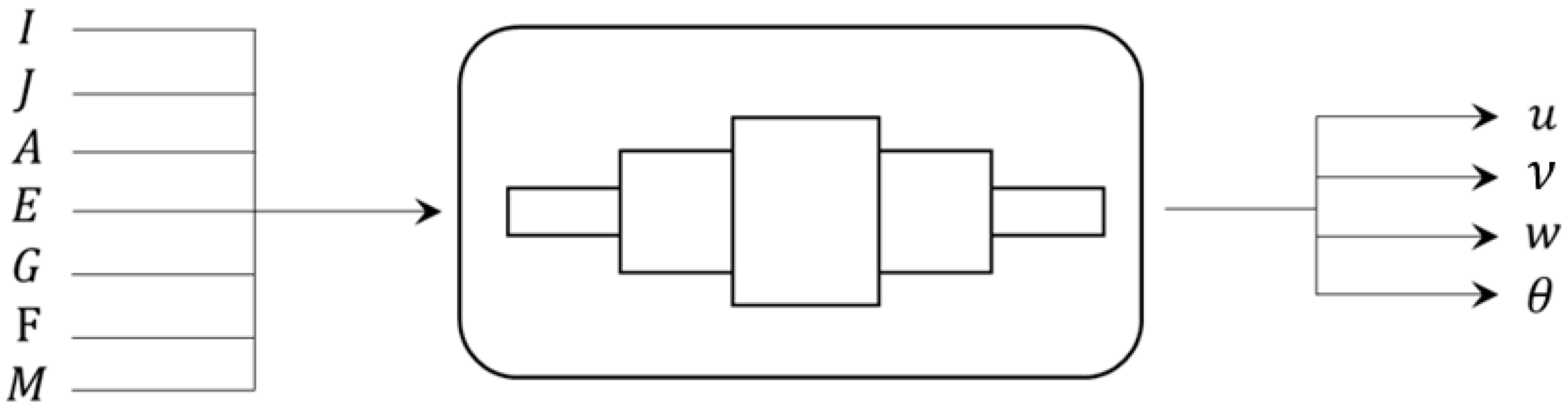
2.3. Shafts
- Shaft geometry: The shaft is divided into n sections, each characterized by its length , inner diameter , and outer diameter ;
- Material properties: Young’s modulus , shear modulus , moment of inertia , polar moment of inertia , and cross-sectional area ;
- Boundary conditions: types of constraints, such as hinges, fixed supports, and bearings;
- Applied loads: radial and axial forces, as well as torques, including forces generated by gears or pulleys.
- Bending
- Torsion
- Stretching
- The deflection must be continuous at every connection point between two segments at the junction . The following equation is enforced:
- The slope must be continuous at transition points, except in the presence of discontinuities in the bending moment (e.g., applied torques):
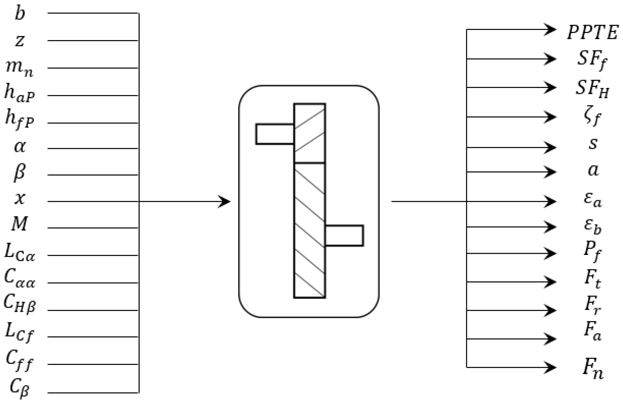
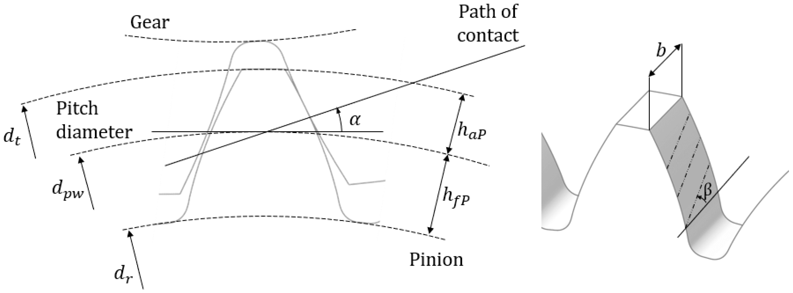
2.4. Gears
- Tangential force:
- Radial force:
- Axial force:
- Normal force:
- Gear body deformation (see Figure 6 for the meaning of the parameters)
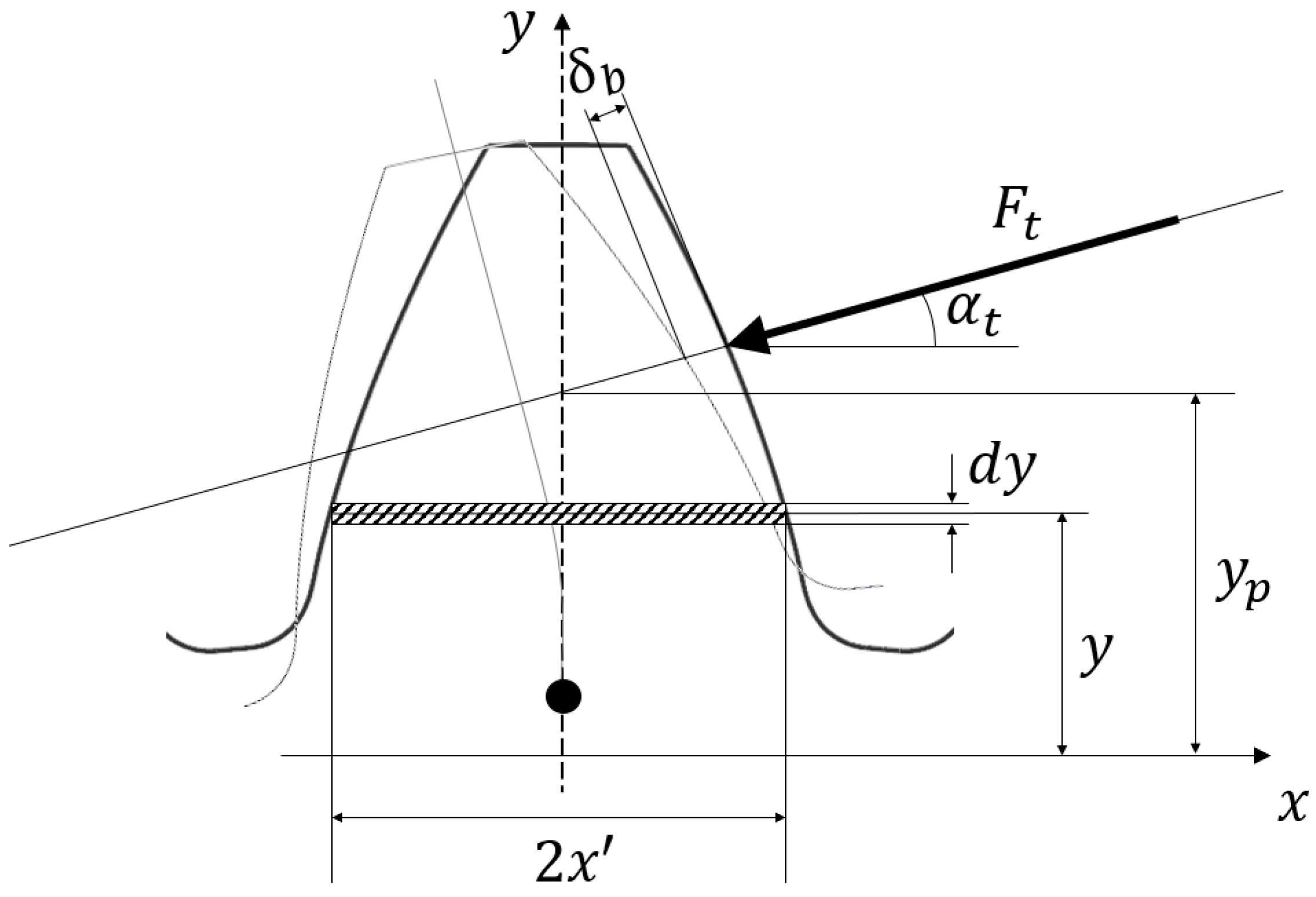
- Tooth bending deformation (see Figure 7 for the meaning of the parameters)
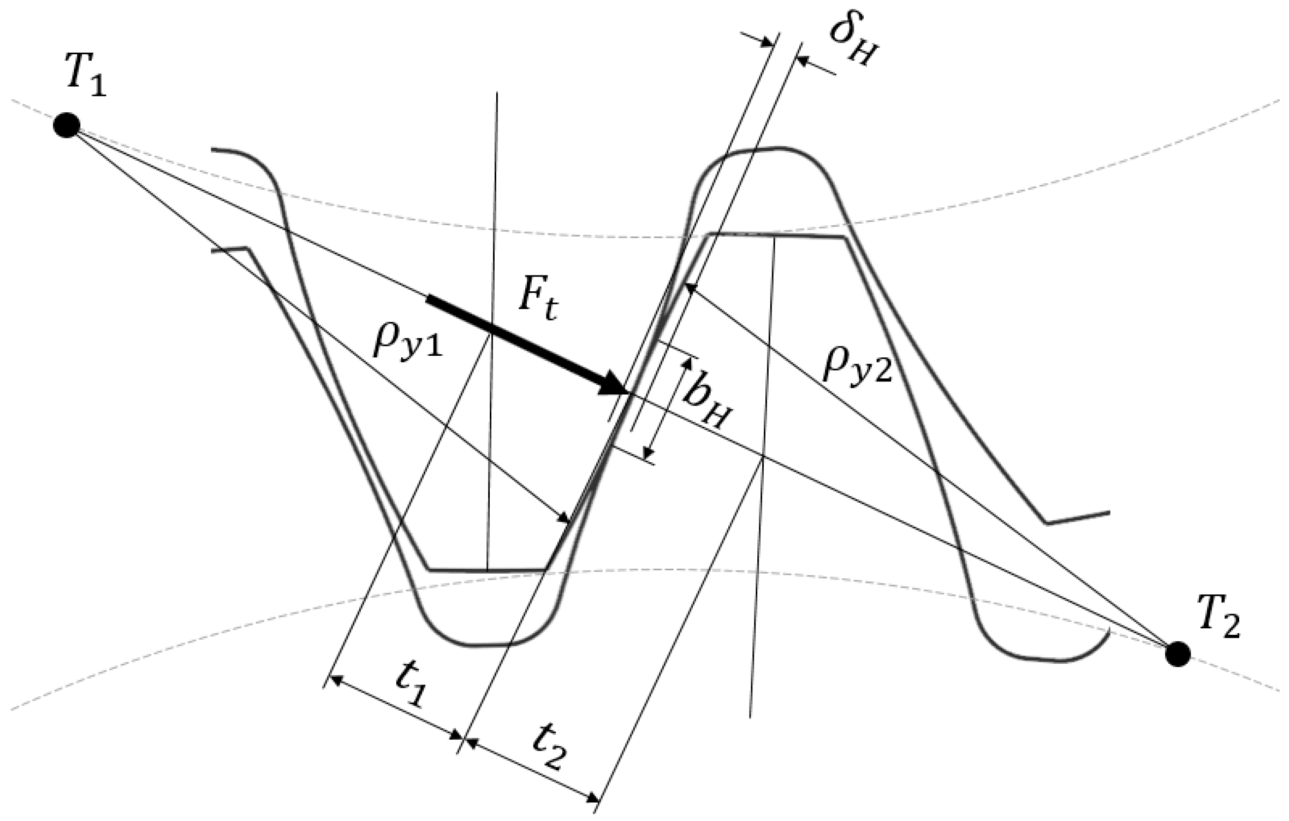
- Contact deformation (see Figure 8 for the meaning of the parameters)
3. Noise Prediction Model
- is the helix angle;
- is the transmission ratio;
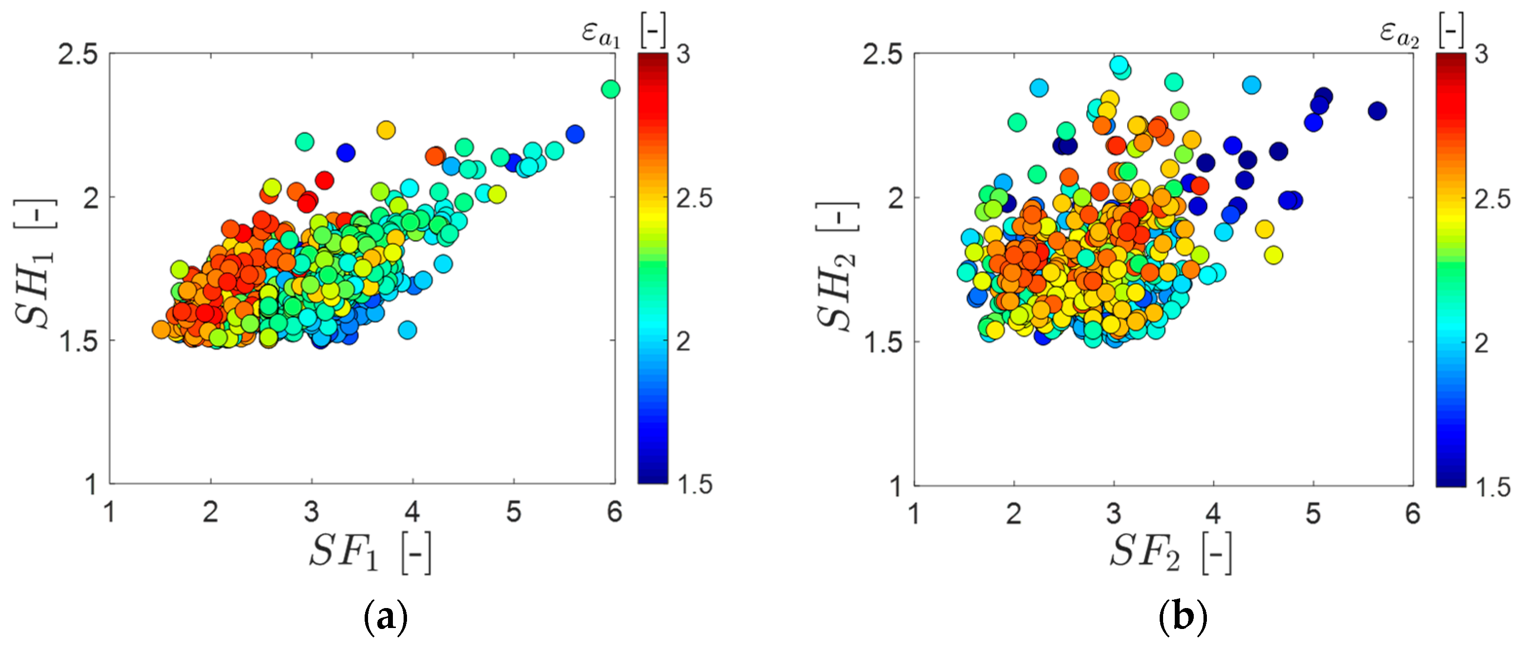
- is the transverse contact ratio;
- is the tangential velocity;
- is the input power;
- is the peak-to-peak static transmission error;
- is the normal tooth force;
- is the effective face width;
- is the mean mesh stiffness.
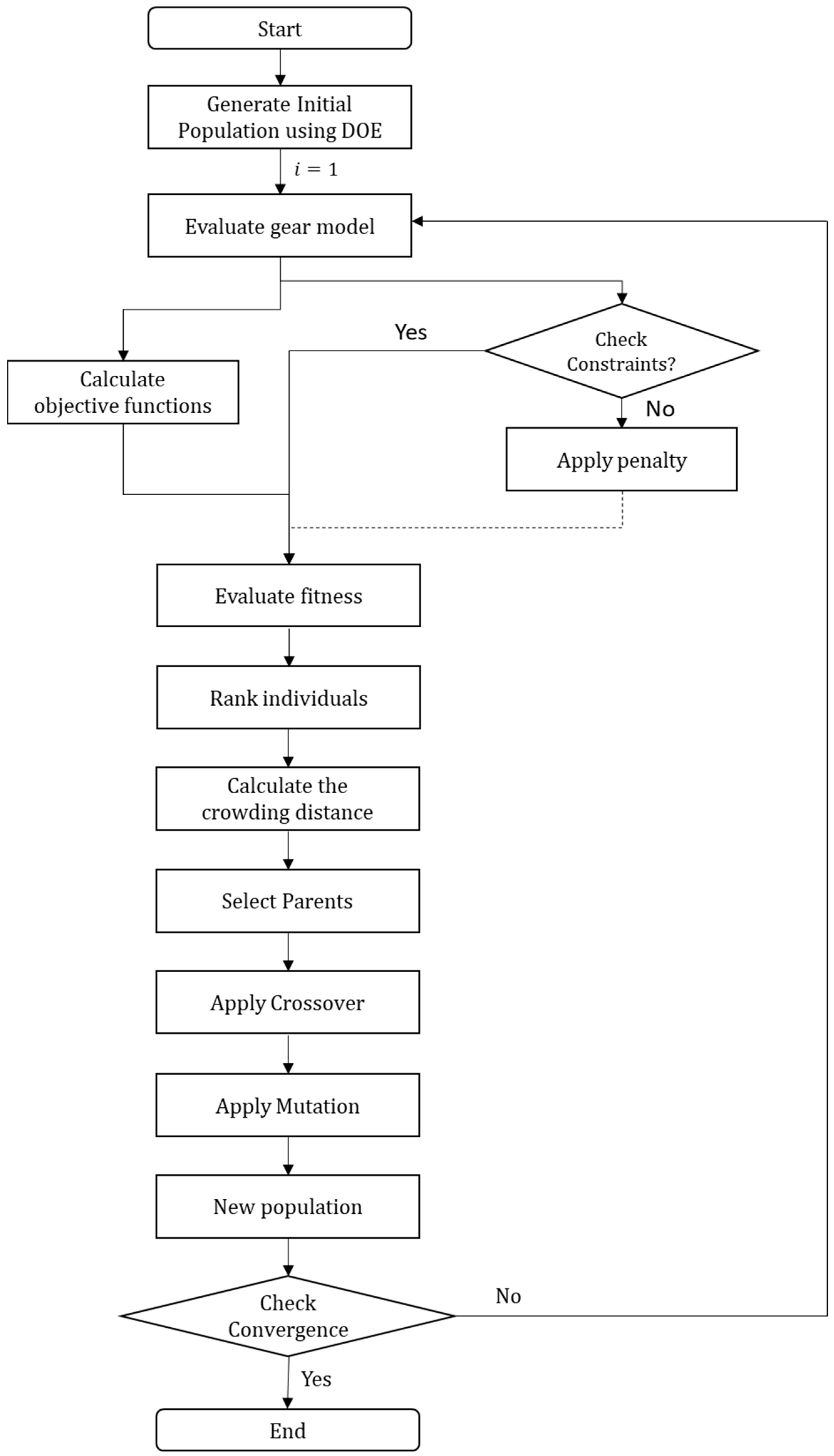
4. Optimization Strategy
- (1)
- Macro-geometry optimization: This phase focuses on identifying a gear configuration that maximizes the contact ratio without compromising structural reliability. The analysis is limited to the gear pair to identify the optimal geometric configuration. Additionally, as this procedure is applied during the design setup phase, it aims to select a configuration that minimizes the center distance, thereby reducing the transmission’s size and friction losses.
- (2)
- Micro-geometry optimization: This phase aims to minimize the peak-to-peak transmission error (PPTE). The analysis requires a detailed study of tooth contact, including the evaluation of shaft deflection and support stiffness, which vary with the applied load. Since the load is inherently nonlinear and iterative, optimizing the macro-geometry first reduces the overall computational complexity before addressing micro-geometry.
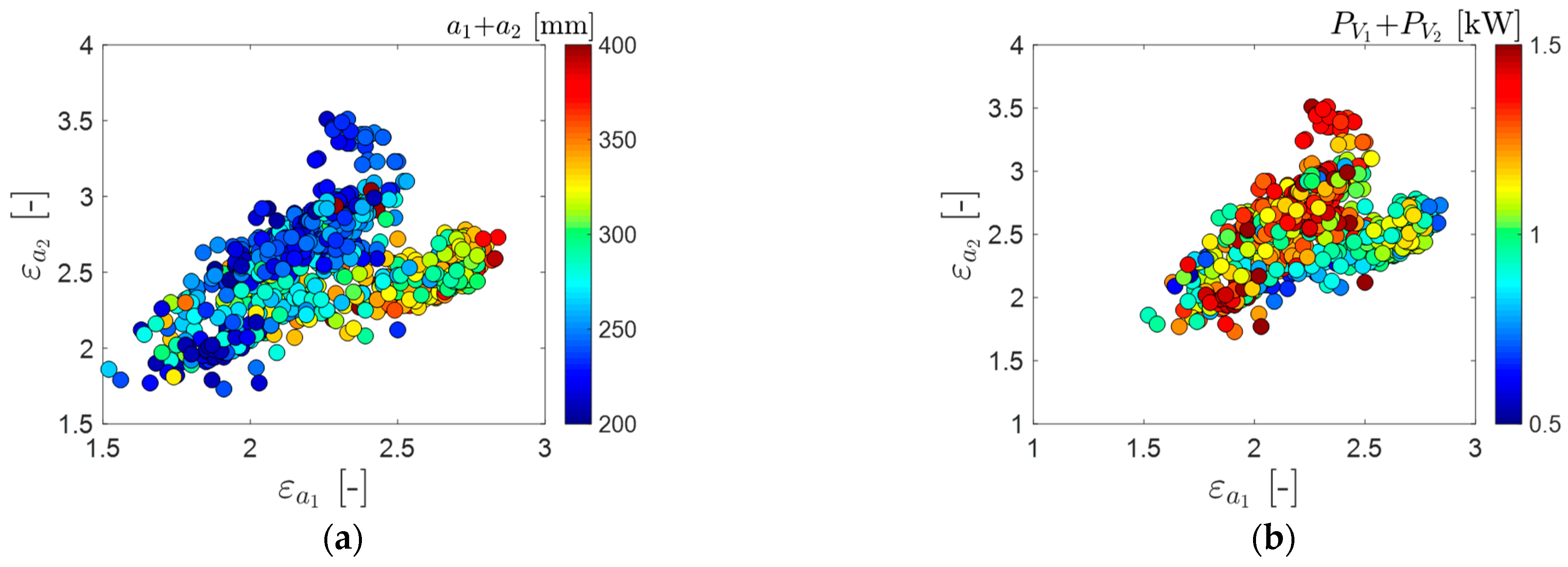
5. Macro-Geometry Optimization Step
6. Micro-Geometry Optimization Step
- Peak–peak of static transmission error ;
- Sound pressure level .
7. Case Study Description and Results
- Four connection bodies: input shaft, idler shaft, output shaft, and ground;
- One driving element: electric motor;
- Two gear couplings;
- Six ball bearings.
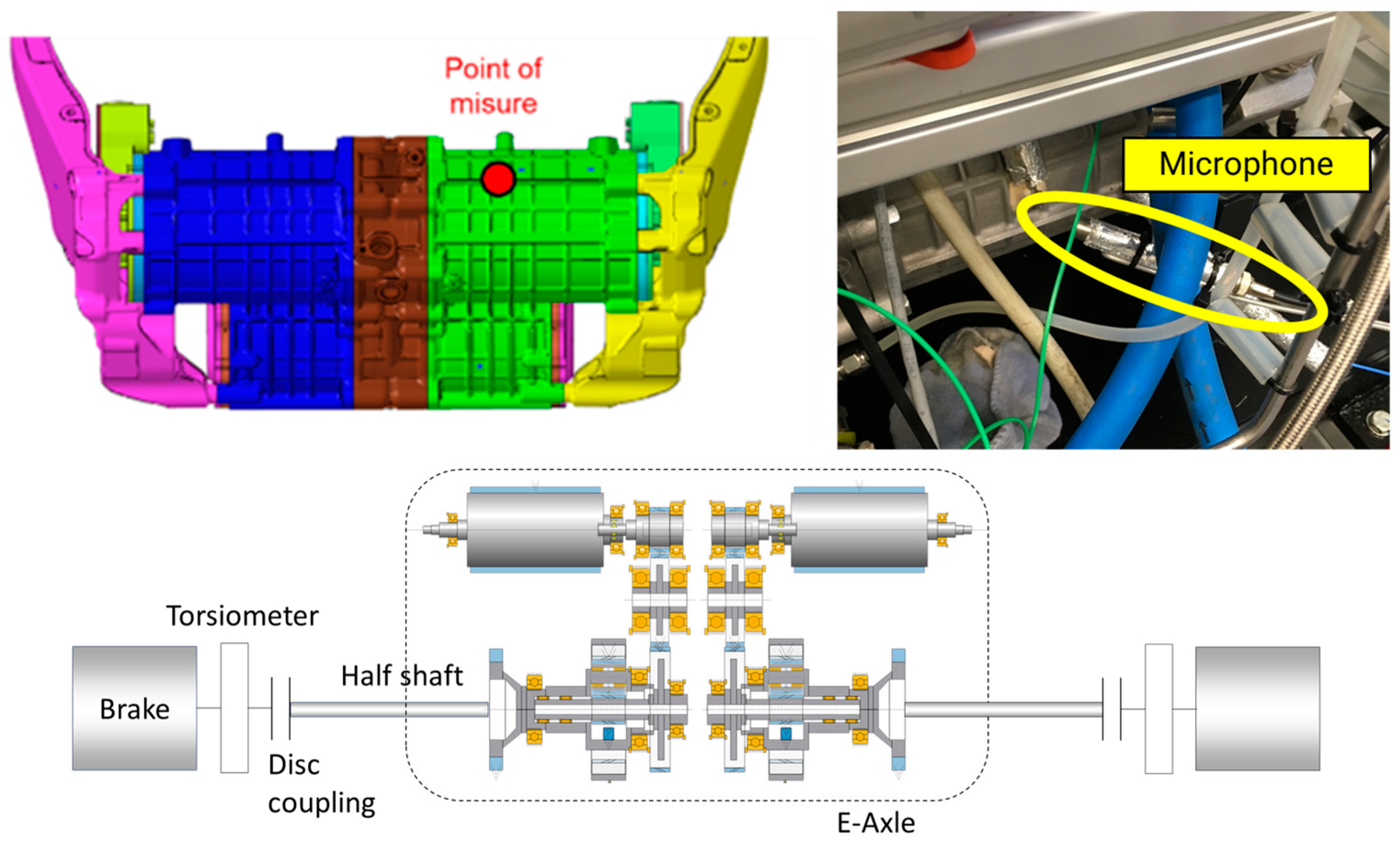
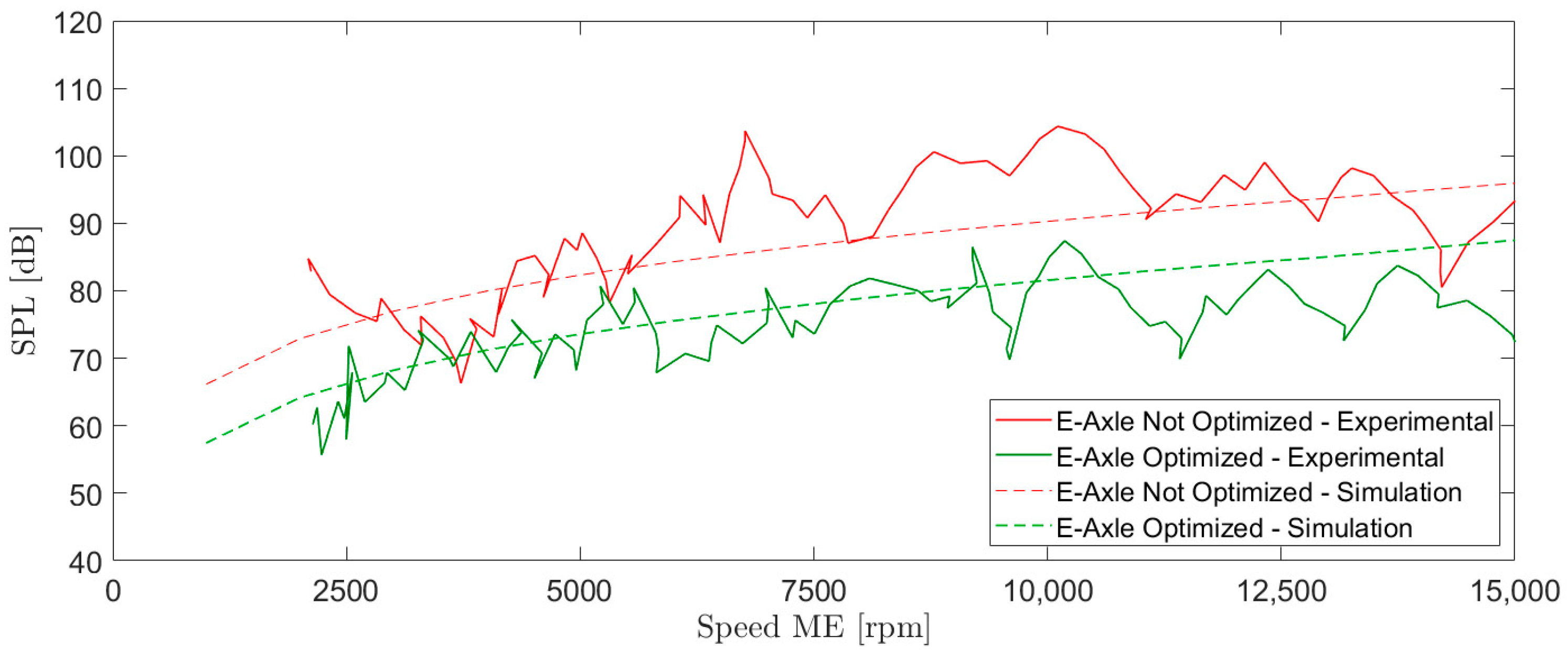
8. Experimental Results, Verification, and Discussion
- Nominal diameter: ½;
- Frequency response characteristic: free-field;
- Frequency range: (±2 dB) 3.5 to 20,000 Hz (3.5 to 20,000 Hz);
- Dynamic range: 138.5 dB re 20 µPa.
- is the distance between the center of the gear and the microphone in Masuda’s model;
- is the distance between the center of the gear and the microphone in the experiment.
9. Conclusions
Author Contributions
Funding
Data Availability Statement
Acknowledgments
Conflicts of Interest
Appendix A
Appendix A.1
- is the zone factor, which takes into account the influence of flank curvatures at the pitch point on Hertzian pressure;
- is the elasticity factor, which takes into account specific properties of the material, moduli of elasticity E, and Poisson’s ratios ν;
- is the contact ratio factor, which takes into account the influence of the effective length of the lines of contact;
- is the helix angle factor, which considers the influence of the helix angle, such as the variation in the load along the lines of contact;
- is the contact ratio of the single stage.
- is the single-pair tooth contact factor that converts contact stress at the pitch point to contact stress at the inner point;
- is the application factor, which takes into account load increments due to externally influenced variations in input or output torque;
- is the dynamic factor, which takes into account load increments due to internal dynamic effects;
- is the face load factor for contact stress, which takes into account the effect of an uneven load distribution over the face width on the contact stress;
- is the transverse load factor for contact stress, which considers uneven load distribution in the transverse direction, resulting, for example, from pitch deviations.
- is the minimum required safety factor for contact stress;
- is the stress limit that is computed according to [49], as a function of the material quality;
- is the lubricant factor, which accounts for the influence of lubricant viscosity on the effect of the lubricant film;
- is the velocity factor, which accounts for the influence of pitch line velocity on the effect of the lubricant film;
- is the roughness factor, which accounts for the influence of surface roughness of the flanks on the effect of the lubricant film;
- is the work hardening factor, which accounts for the effect of meshing with a surface-hardened or similarly hard mating gear;
- is the size factor relevant to contact stress, which considers the influence of tooth dimensions on the permissible contact stress;
- is the life factor for test gears for contact stress. It considers the higher load capacity for a limited number of load cycles.
Appendix A.2
- is the form factor, which takes into account the influence on nominal tooth root stress of the tooth form, with load applied at the outer point of single pair tooth contact;
- is the stress concentration factor, which is used to convert the nominal tooth root stress to local tooth root stress. It takes into account the stress-amplifying effect of section change at the filet radius at tooth root;
- is the helix angle factor, which compensates for the fact that the bending moment intensity at the tooth root of helical gears is—as a consequence of the oblique lines of contact—less than the corresponding value for the virtual spur gears used as the bases for calculation;
- is the rim thickness factor, which adjusts the calculated tooth root stress for thin rimmed gears;
- is the deep tooth factor, which adjusts the calculated tooth root stress for high precision gears with a high contact ratio .
- is the nominal tooth root stress, which is the maximum local principal stress produced at the tooth root when a gear pair is loaded by the static nominal torque;
- is the application factor, which takes into account load increments due to externally influenced variations in input or output torque;
- is the dynamic factor, which takes into account load increments due to internal dynamic effects;
- is the face load factor for tooth root stress, which considers the effect of an uneven load distribution over the face width on the stresses at the tooth root. The uneven load distribution is due to mesh misalignment caused by inaccuracies in manufacture, elastic deformations and so on;
- is the transverse load factor for tooth root stress, which considers uneven load distribution in the transverse direction.
- is the minimum required safety factor for tooth root stress;
- is the limit stress and the value can be retrieved from [49], as a function of the material quality and the core hardness;
- is the stress correction factor, depending on the standard reference test gear used to characterize the material;
- is the alternating bending factor, whose value depends on the gear working conditions [50];
- is the relative notch sensitivity factor. It is the ratio between the notch sensitivity factor of the gear of interest and the standard test gear factor; it does not show any significant dependence with respect to the number of cycles;
- is the relative surface factor. It is the ratio between the surface roughness factor of tooth root filets of the gear of interest and the toot root filet factor of the reference test gear; it does not show any significant dependence with respect to the number of cycles;
- is the size factor relevant to tooth strength, which is used to consider the influence of tooth dimensions on tooth bending strength. Its value depends on the normal module and on the material;
- is the life factor for tooth root stress. It considers the higher load capacity for a limited number of load cycles. In practice, this is the parameter which makes the permissible stress dependent on the number of cycles.
Appendix A.3
References
- Gissel, M.; Nielsen, A.F. Influence of gear tooth geometry on the noise and vibration of gears. J. Sound Vib. 2000, 238, 381–395. [Google Scholar]
- Rosso, C.; Bruzzone, F.; Maggi, T.; Marcellini, C. Influence of Micro Geometry Modification on Gear Dynamics; SAE Technical Paper 2020-01-1323; SAE International: Warrendale, PA, USA, 2020. [Google Scholar]
- Stroud, I.R.; Hartley, P.F. The effect of gear surface finish on noise and vibration performance. Proc. Inst. Mech. Eng. Part C J. Mech. Eng. Sci. 2001, 2015, 1261–1270. [Google Scholar]
- Choi, W.; Lee, C.H. Effect of manufacturing errors on the vibration characteristics of gears. J. Mech. Des. 2018, 32, 2107–2114. [Google Scholar]
- Kahraman, A.; Blankenship, G.W. Effect of Involute Contact Ratio on Spur Gear Dynamics. J. Mech. Des. 1999, 121, 112–118. [Google Scholar] [CrossRef]
- Sato, T.; Umezawa, K.; Ishikawa, J. Effects of Contact Ratio and Profile Correction on Gear Rotational Vibration. Bull. JSME 1983, 26, 2010–2016. [Google Scholar] [CrossRef]
- Staph, H.E. A Parametric Analysis of High-Contact-Ratio Spur Gears. A S L E Trans. 1976, 19, 201–215. [Google Scholar] [CrossRef]
- Cornell, R.W.; Westervelt, W.W. Dynamic Tooth Loads and Stressing for High Contact Ratio Spur Gears. J. Mech. Des. 1978, 100, 69–76. [Google Scholar] [CrossRef]
- Anderson, N.E.; Loewenthal, S.H. Efficiency of Nonstandard and High Contact Ratio Involute Spur Gears. J. Mech. Trans. Autom. 1986, 108, 119–126. [Google Scholar] [CrossRef]
- Ozguven, H.; Houser, D. Mathematical models used in gear dynamics—A review. J. Sound Vib. 1988, 121, 383–411. [Google Scholar] [CrossRef]
- Chang, L.; Liu, G.; Wu, L. A robust model for determining the mesh stiffness of cylindrical gears. Mech. Mach. Theory 2015, 87, 93–114. [Google Scholar] [CrossRef]
- Kahraman, A.; Blankenship, G. Gear dynamics experiments, Part-I: Characterization of forced response. In Proceedings of the ASME 6th Power Transmission and Gearing Conference Phoenix, Phoenix, AZ, USA, 13–16 September 1996. [Google Scholar]
- Cirelli, M.; Valentini, P.P.; Pennestrì, E. A study of the non-linear dynamic response of spur gear using a multibody contact based model with flexible teeth. J. Sound Vib. 2019, 445, 148–167. [Google Scholar] [CrossRef]
- Kahraman, A.; Blankenship, G.W. Effect of Involute Tip Relief on Dynamic Response of Spur Gear Pairs. J. Mech. Des. 1999, 121, 313–315. [Google Scholar] [CrossRef]
- Cirelli, M.; Giannini, O.; Valentini, P.P.; Pennestrì, E. Influence of tip relief in spur gears dynamic using multibody models with movable teeth. Mech. Mach. Theory 2020, 152, 103948. [Google Scholar] [CrossRef]
- Autiero, M.; Paoli, G.; Cirelli, M.; Valentini, P.P. The effect of different profile modifications on the static and dynamic transmission error of spur gears. Mech. Mach. Theory 2024, 201, 105752. [Google Scholar] [CrossRef]
- Munro, R.G.; Palmer, D.; Morrish, L. An experimental method to measure gear tooth stiffness throughout and beyond the path of contact. Proc. Inst. Mech. Eng. Part C J. Mech. Eng. Sci. 2001, 215, 793–803. [Google Scholar] [CrossRef]
- Palermo, A.; Britte, L.; Janssens, K.; Mundo, D.; Desmet, W. The measurement of Gear Transmission Error as an NVH indicator: Theoretical discussion and industrial application via low-cost digital encoders to an all-electric vehicle gearbox. Mech. Syst. Signal Process. 2018, 110, 368–389. [Google Scholar] [CrossRef]
- Kahraman, A.; Tamminana, V.; Vijayakar, S. A Study of the Relationship Between the Dynamic Factors and the Dynamic Transmission Error of Spur Gear Pairs. J. Mech. Des. 2007, 129, 75–84. [Google Scholar]
- Cirelli, M.; Autiero, M.; Belfiore, N.P.; Paoli, G.; Pennestrì, E.; Valentini, P.P. Review and comparison of empirical friction coefficient formulation for multibody dynamics of lubricated slotted joints. Multibody Syst. Dyn. 2024, 63, 83–104. [Google Scholar] [CrossRef]
- Autiero, M.; Cera, M.; Cirelli, M.; Pennestrì, E.; Valentini, P.P. Review with Analytical-Numerical Comparison of Contact Force Models for Slotted Joints in Machines. Machines 2022, 10, 966. [Google Scholar] [CrossRef]
- Lohmann, C.; Walkowiak, M.; Tenberge, P. Optimal modifications on helical gears for good load distribution and minimal wear. In Proceedings of the International Gear Conference 2014, Lyon, France, 26–28 August 2014. [Google Scholar]
- Autiero, M.; Cirelli, M.; Paoli, G.; Valentini, P.P. A Data-Driven Approach to Estimate the Power Loss and Thermal Behaviour of Cylindrical Gearboxes under Transient Operating Conditions. Lubricants 2023, 11, 303. [Google Scholar] [CrossRef]
- Abdelounis, H.B.; Bot, A.L.; Liaudet, J.P.; Zahouani, H. An experimental study on roughness noise of dry rough flat surfaces. Wear 2010, 268, 335–345. [Google Scholar] [CrossRef]
- Chung, W.-J.; Park, Y.-J.; Choi, C.; Kim, S.-C. Effects of manufacturing errors of gear macro-geometry on gear performance. Sci. Rep. 2023, 13, 50. [Google Scholar] [CrossRef]
- Geradts, P.; Brecher, C.; Löpenhaus, C.; Kasten, M. Reduction of the tonality of gear noise by application of topography scattering. Appl. Acoust. 2019, 148, 344–359. [Google Scholar] [CrossRef]
- Ben Younes, E.; Changenet, C.; Bruyère, J.; Rigaud, E.; Perret-Liaudet, J. Multi-objective optimization of gear unit design to improve efficiency and transmission error. Mech. Mach. Theory 2022, 167, 104499. [Google Scholar] [CrossRef]
- Choi, C.; Ahn, H.; Yu, J.; Han, J.-S.; Kim, S.-C.; Park, Y.-J. Optimization of gear macro-geometry for reducing gear whine noise in agricultural tractor transmission. Comput. Electron. Agric. 2021, 188, 106358. [Google Scholar] [CrossRef]
- Kim, S.-C.; Moon, S.-G.; Sohn, J.-H.; Park, Y.-J.; Choi, C.-H.; Lee, G.-H. Macro geometry optimization of a helical gear pair for mass, efficiency, and transmission error. Mech. Mach. Theory 2020, 144, 103634. [Google Scholar] [CrossRef]
- Choi, C.; Ahn, H.; Park, Y.-J.; Lee, G.-H.; Kim, S.-C. Influence of gear tooth addendum and dedendum on the helical gear optimization considering mass, efficiency, and transmission error. Mech. Mach. Theory 2021, 166, 104476. [Google Scholar] [CrossRef]
- Korta, J.A.; Mundo, D. Multi-objective micro-geometry optimization of gear tooth supported by response surface methodology. Mech. Mach. Theory 2017, 109, 278–295. [Google Scholar] [CrossRef]
- Garambois, P.; Perret-Liaudet, J.; Rigaud, E. NVH robust optimization of gear macro and microgeometries using an efficient tooth contact model. Mech. Mach. Theory 2017, 117, 78–95. [Google Scholar] [CrossRef]
- Mohammed, O.D.; Bhat, A.D.; Falk, P. Robust multi-objective optimization of gear microgeometry design. Simul. Model. Pract. Theory 2022, 119, 102593. [Google Scholar] [CrossRef]
- Marafona, J.D.; Carneiro, G.N.; Marques, P.M.; Martins, R.C.; António, C.C.; Seabra, J.H. Gear design optimization: Stiffness versus dynamics. Mech. Mach. Theory 2024, 191, 105503. [Google Scholar] [CrossRef]
- Yang, J.-X.; Chen, Z.-Y.; Shi, W.-K.; Yang, H.-B.; Liu, J.; Yuan, R.-F.; Zhao, Y.-Y.; Dong, Y.-H. Robust modification optimization for helical gear mounting errors based on contact ratio. Measurement 2024, 237, 115196. [Google Scholar] [CrossRef]
- Dixit, Y.; Kulkarni, M.S. Multi-objective optimization with solution ranking for design of spur gear pair considering multiple failure modes. Tribol. Int. 2023, 180, 108284. [Google Scholar] [CrossRef]
- Masuda, T.; Abe, T.; Hattori, K. Prediction Method of Gear Noise Considering the Influence of the Tooth Flank Finishing Method. J. Vib. Acoust. 1986, 108, 95–100. [Google Scholar] [CrossRef]
- ISO 16281; Rolling Bearings–Methods for Calculating the Modified Reference Rating Life for. International Organization for Standardization: Geneva, Switzerland, 2025.
- Weber, C. The Deformations of Loaded Gears and the Effect on Their Load-Carrying Capacity; Report No.3; British Department of Scientific and Industrial Research: London, UK, 1949. [Google Scholar]
- Mengjiao, F.; Ma, H.; Zhanwei, L.; Wang, Q.; Wen, B. An improved analytical method for calculating time-varying mesh stiffness of helical gears. Meccanica 2017, 53, 1131–1145. [Google Scholar]
- ISO 6336-2; Calculation of Surface Durability (Pitting). International Organization for Standardization: Geneva, Switzerland, 2007.
- ISO 6336-3; Calculation of Tooth Bending Strength. International Organization for Standardization: Geneva, Switzerland, 2007.
- BS ISO/TR 14179-2:2001; Gears-Thermal Capacity—Part 2: Thermal Load Carrying Capacity. British Standards Institution: London, UK, 2001.
- Deb, K.; Pratap, A.; Agarwal, S.; Meyarivan, T. A fast and elitist multiobjective genetic algorithm: NSGA-II. IEEE Trans. Evol. Comput. 2002, 6, 182–197. [Google Scholar] [CrossRef]
- Skrickij, V.; Bogdevičius, M. Vehicle gearbox dynamics: Centre distance influence on mesh stiffness and spur gear dynamics. Transport 2010, 25, 278–286. [Google Scholar] [CrossRef]
- Luo, Y.; Baddour, N.; Liang, M. Effects of gear center distance variation on time varying mesh stiffness of a spur gear pair. Eng. Fail. Anal. 2017, 75, 37–53. [Google Scholar] [CrossRef]
- ISO 6336-1; Basic Principles, Introduction and General Influence Factors. International Organization for Standardization: Geneva, Switzerland, 2007.
- Del Pio, G.; Pennestrì, E.; Valentini, P.P. Kinematic and power-flow analysis of bevel gears planetary gear trains with gyroscopic complexity. Mech. Mach. Theory 2013, 70, 523–537. [Google Scholar] [CrossRef]
- ISO 6336-5; Strength and Quality of Materials. International Organization for Standardization: Geneva, Switzerland, 2007.
- Linke, H. Stirnradverzahnung. Berechnung. Werkstoffe. Fertigung; Carl Hanser-Verlag: München, Germany, 1996. [Google Scholar]


| Input | Output | ||||
|---|---|---|---|---|---|
| Speed | [rpm] | Torque | [Nm] | ||
| Input | Output | ||||
|---|---|---|---|---|---|
| Internal raceway groove curvature radius | [mm] | Stiffness | [N/m] | ||
| External raceway groove curvature radius | [mm] | Deflection | [mm] | ||
| Ball diameter | [mm] | ||||
| Bearing pitch diameter | [mm] | ||||
| Contact angle | [°] | ||||
| Normal load | [N] | ||||
| Input | Output | ||||
|---|---|---|---|---|---|
| Moment of inertia | [] | Axial displacement | |||
| Polar moment of inertia | [] | Vertical displacement | |||
| Area | [] | Transverse displacement | |||
| Young modulus | [] | Torsion angle | |||
| Shear modulus | [] | ||||
| Applied torque | [] | ||||
| Input | Output | ||||
|---|---|---|---|---|---|
| Face width | Peak–peak static transmission error | ] | |||
| Number of teeth | [-] | Tooth bending strength | [-] | ||
| Normal module | Tooth pitting resistance | [-] | |||
| Addendum | Specific sliding | [°] | |||
| Dedendum | Center distance | ||||
| Pressure angle | Transverse contact ratio | [-] | |||
| Helix angle | Axial contact ratio | [-] | |||
| Correction factor | [-] | Total power loss | |||
| Torque | M | Tangential force | [N] | ||
| Tip relief length | Radial force | [N] | |||
| Tip relief amplitude | Axial force | [N] | |||
| Flank line slope modification | Normal force | [N] | |||
| Root relief length | |||||
| Root relief amplitude | |||||
| Flank line crowning | |||||
| Input | Optimization Variables | Constraints | Objective Functions |
|---|---|---|---|
| Electric machine power | Normal module | Tooth bending strength ≥ 1.5 | Center-to-center distance |
| Overall transmission ratio | Pressure angle | Tooth pitting resistance ≥ 1.5 | Transverse contact ratio |
| Helix angle | Specific sliding ≤ 3 | Total power loss | |
| Addendum factor | |||
| Dedendum factor | |||
| Number of teeth | |||
| Correction factor | |||
| Face width |
| Input | Optimization Variables | Constraints | Objective Functions |
|---|---|---|---|
| Initial/Reference | Optimized | |||||||
|---|---|---|---|---|---|---|---|---|
| Pinion | Idler | Output | Pinon | Idler | Output | |||
| Torque | [Nm] | 85 | 201 | 292 | 85 | 183 | 251 | |
| Speed | [rpm] | 10,000 | 4210 | 2909 | 10,000 | 4651 | 3389 | |
| Normal module | [mm] | 2.0 | 2.0 | 2.0 | 1.8 | 1.8 | 1.8 | |
| Pressure angle | [°] | 20 | 20 | 20 | 20 | 20 | 20 | |
| Helix angle | [°] | 28.5 | 28.5 | 28.5 | 28.5 | 28.5 | 28.5 | |
| Addendum factor | [mm] | 2.869 | 2.889 | 2.868 | 1.20 | 1.50 | 1.50 | |
| Dedendum factor | [mm] | 2.431 | 2.811 | 2.932 | 1.80 | 1.80 | 1.80 | |
| Number of teeth | [-] | 16 | 38 | 55 | 20 | 43 | 59 | |
| Correction factor | [-] | 0.407 | 0.150 | 0.092 | 0.390 | 0 | −0.359 | |
| Face width | [mm] | 13 | 14 | 13 | 20 | 18 | 19.9 | |
| Center distance | [mm] | 62.5 106.3 | 65.2 103.8 | |||||
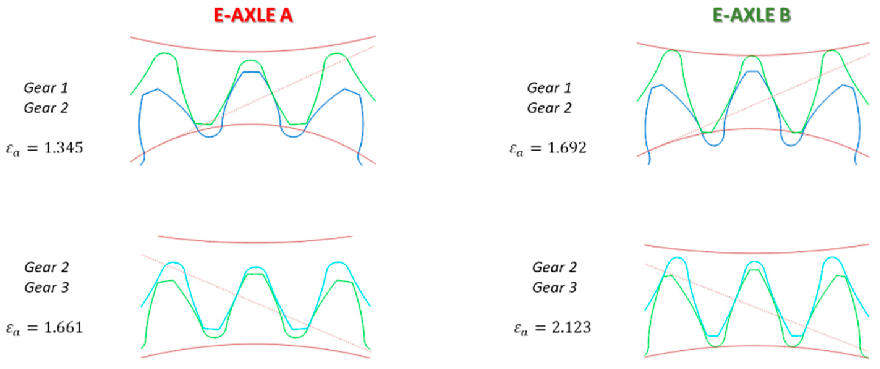
| Transverse contact ratio | [-] | 1.345 1.661 | 1.692 2.123 | |||||
| Power loss | [kW] | 0.85 0.45 | 0.80 0.50 | |||||
Disclaimer/Publisher’s Note: The statements, opinions and data contained in all publications are solely those of the individual author(s) and contributor(s) and not of MDPI and/or the editor(s). MDPI and/or the editor(s) disclaim responsibility for any injury to people or property resulting from any ideas, methods, instructions or products referred to in the content. |
© 2025 by the authors. Licensee MDPI, Basel, Switzerland. This article is an open access article distributed under the terms and conditions of the Creative Commons Attribution (CC BY) license (https://creativecommons.org/licenses/by/4.0/).
Share and Cite
Cianciotta, L.; Cirelli, M.; Valentini, P.P. Multi-Objective Optimization of Gear Design of E-Axles to Improve Noise Emission and Load Distribution. Machines 2025, 13, 330. https://doi.org/10.3390/machines13040330
Cianciotta L, Cirelli M, Valentini PP. Multi-Objective Optimization of Gear Design of E-Axles to Improve Noise Emission and Load Distribution. Machines. 2025; 13(4):330. https://doi.org/10.3390/machines13040330
Chicago/Turabian StyleCianciotta, Luciano, Marco Cirelli, and Pier Paolo Valentini. 2025. "Multi-Objective Optimization of Gear Design of E-Axles to Improve Noise Emission and Load Distribution" Machines 13, no. 4: 330. https://doi.org/10.3390/machines13040330
APA StyleCianciotta, L., Cirelli, M., & Valentini, P. P. (2025). Multi-Objective Optimization of Gear Design of E-Axles to Improve Noise Emission and Load Distribution. Machines, 13(4), 330. https://doi.org/10.3390/machines13040330