Decentralized Adaptive Control of Closed-Kinematic Chain Mechanism Manipulators

Abstract

This paper presents a new decentralized adaptive control scheme for motion control of robot manipulators built based on a closed-kinematic chain mechanism (CKCM). By employing the synchronization technique and model reference adaptive control (MRAC) based on the Lyapunov direct method, the Decentralized Adaptive Synchronized Control scheme (DASCS) is developed. The DASCS can ensure global asymptotic convergence of tracking errors while forcing all active joints to move in a predefined synchronous manner in the presence of uncertainties and sudden changes in payload. Furthermore, the control scheme has a simple structure, independent of the manipulator’s dynamic model, ensuring computational efficiency. Results of computer simulations conducted to evaluate the performance of the control scheme applied to controlling the motion of a CKCM manipulator with six degrees of freedom are reported and discussed.

1. Introduction

Robot manipulators whose structure assumes a closed-kinematic chain mechanism (CKCM) have attracted great attention from robotic researchers due to their advantages over their counterparts, namely manipulators with open kinematic chain mechanisms (OKCM) [1,2]. CKCM manipulators can mitigate the weaknesses of OKCM manipulators such as low stiffness, poor stability, small payload, and accumulated and amplified errors from link to link [3,4]. The CKCM was first employed in the design and construction of the Stewart Platform (SP), which possesses six degrees of freedom (DOF) [5]. Nowadays, the SP has a wide application area in spacecraft simulation, vehicle dynamics, high-speed train dynamics, airplane dynamics, drone manipulation, medical rehabilitation, and high-speed assembly operation [6,7,8].

In order for a robot to track a desired trajectory, a closed-loop feedback controller employs sensors to gain awareness of its surroundings and then adjusts the appropriate control strategy to achieve a desired performance, much like the way a human brain works. In general, robotic systems are complicated, time-varying, and highly nonlinear systems with uncertainties and disturbances in their working environment [9]. Moreover, due to the closed-loop structure of CKCM manipulators, the motion of each active joint is constrained by the motion of other active joints. Thus, the lack of synchronization between active joints will lead to a large coupling effect, which degrades the performance of the whole system or even damages its mechanical structure, especially at high speeds and with large payloads. Therefore, it is essential for a CKCM manipulator to possess a synchronized controller that has the capacity to adapt and improve itself under changing conditions without human intervention and to force each active joint to follow its desired trajectory as close as possible while synchronizing its motion with the other active joints’ motions in a defined, synchronous manner.

Recently, a synchronization method based on cross-coupling control technology has been developed to solve the abovementioned problem by allowing each control loop to receive feedback from itself as well as from the others to achieve better coordination and then improve the manipulator performance significantly [10]. This approach is a powerful tool for not only CKCM manipulators but also systems that require multiple objects to operate simultaneously to achieve a common goal, such as swarms of mobile robot [11,12] or multiple robotic manipulator systems [13,14,15]. While the work in reference [10], dealing with cross-coupled control of biaxial systems in which an error in an axis impacts the control loops of both axes, is a time-based approach, the recently introduced method for synchronization in reference [16] is based on position domain. The authors in reference [16] introduced a position-domain control method rather than a time-domain one to enhance contour tracking performance of a multi-axis motion system. The synchronization of the axes is achieved by formulating the motion system as a master-slave motion system in which the master motion is used as an independent variable and the slave motions are expressed as functions of the master motion according to the required contour trajectories.

Most existing synchronized control schemes are model-based adaptive control schemes [17,18] and their implementation requires a precise dynamical model of the manipulator [19,20,21]. Due to the fact that it is difficult if not impossible to acquire a precise dynamical model of the manipulator and that its associated mathematical calculation is computationally intensive, these synchronized control schemes are not suitable for real-time applications in CKCM manipulators, particularly for those with more than 2 DOFs. To tackle the above dynamic modelling issue, robotics researchers have considered intelligent approaches such as fuzzy logic [22,23] and artificial neural network control schemes [24,25,26]. However, these intelligent controllers exhibited shortcomings such as assurance of stability, high computational demand, slow convergence rate, and time-consuming training process. Finally, the authors in references [27,28,29] considered synchronized control schemes that have simple structures and do not require the knowledge of the manipulator dynamics in the implementation of their control laws. However, their controller gains must still be selected based on conservative estimates of the manipulator dynamic model, which could be problematic and impractical.

During the trajectory tracking processes, CKCM manipulators can be treated as a group of multi OKCM manipulators holding the same payload. Hence, it is possible to develop a decentralized control scheme in which each active joint is controlled independently to minimize the computational cost and move synchronously to achieve the desired tracking performance of the moving platform [29].

In this paper, we develop a new decentralized adaptive synchronized control scheme (DASCS) for CKCM manipulators. Unlike conventional decentralized control schemes [30], each sub-controller of the DASCS receives feedback from not only its active joint but also from two neighboring ones. Compared to the work in references [10,16], the DASCS developed in the present paper is a time-domain approach providing synchronization of one particular joint with its two neighboring joints, while the work in reference [10] dealt with synchronization of two axes and the work in reference [16] is a position-domain approach. Then, by applying the model reference adaptive control (MRAC) technique based on the Lyapunov direct method into the synchronized control method, the DASCS guarantees the global asymptotic convergence of tracking errors to zero while synchronizing all active joints’ motion and overcoming uncertainties and disturbances. Moreover, the DASCS, whose controller gains are updated by an adaptation law driven only by the actual and desired trajectories of active joints, is computationally efficient and thus is suitable for real-time applications.

The structure of this paper is as follows. Section 2 describes the synchronization control method and Section 3 presents the development of the DASCS. Section 4 presents and discusses the results of a computer simulation study conducted to evaluate the effectiveness of the DASCS in comparison with another existing adaptive control scheme. Section 5 concludes the paper with summary and future research directions.

2. Synchronization Control

For a CKCM manipulator with $n$ active joints, to achieve synchronization, we define the following relationship:

$${\displaystyle \frac{q_1\left(t\right)}{q_{d1}\left(t\right)}}={\displaystyle \frac{q_2\left(t\right)}{q_{d2}\left(t\right)}}=\cdots ={\displaystyle \frac{q_n\left(t\right)}{q_{dn}\left(t\right)}}$$

(1)

where $q_{di}$ and $q_i\left(t\right)$ denote the desired and actual trajectory of the ith active joint, respectively.

If all ratios in (1) are equal, or in other words, if Equation (1) is valid, then all active joints will move in a synchronous manner [27]. However, considering synchronization of all active joints may lead to a heavy computational burden, especially when the number of active joints is large.

To avoid synchronization of all active joints, we proceed to rewrite (1) as a set of subgoals:

$${\displaystyle \frac{q_i\left(t\right)}{q_{di}\left(t\right)}}={\displaystyle \frac{q_{i+1}\left(t\right)}{q_{di+1}\left(t\right)}}$$

(2)

From subgoals (2), synchronization functions are defined as follows:

$$\left\{\begin{array}{c}{f}_1\left[q_1\left(t\right),q_2\left(t\right)\right]={\displaystyle \frac{q_1\left(t\right)}{q_{d1}}}-{\displaystyle \frac{q_2\left(t\right)}{q_{d2}}}=0\\ f_2\left[q_2\left(t\right),q_3\left(t\right)\right]={\displaystyle \frac{q_2\left(t\right)}{q_{d2}\left(t\right)}}-{\displaystyle \frac{q_3\left(t\right)}{q_{d3}\left(t\right)}}=0\\ ⋮\\ f_i\left[q_i\left(t\right),q_{i+1}\left(t\right)\right]={\displaystyle \frac{q_i\left(t\right)}{q_{di}\left(t\right)}}-{\displaystyle \frac{q_{i+1}\left(t\right)}{q_{di+1}\left(t\right)}}=0\\ ⋮\\ f_n\left[q_n\left(t\right),q_1\left(t\right)\right]={\displaystyle \frac{q_n\left(t\right)}{q_{dn}\left(t\right)}}-{\displaystyle \frac{q_1\left(t\right)}{q_{d1}\left(t\right)}}=0\end{array}\right.$$

(3)

We use Taylor Series [31] to expand (3) at the desired joint trajectories $q_{di}(t$) to obtain the following:

$$\begin{array}{c}{f}_i\left[q_i\left(t\right),q_{i+1}\left(t\right)\right]=f_i\left[q_{di}\left(t\right),q_{di+1}\left(t\right)\right]+{\displaystyle \sum _{j=i}^{j=i+1}}\begin{array}{c}\left[\left.{\displaystyle \frac{\partial f_i\left(.\right)}{\partial q_j}}\right|\right]\\ { q}_{di}\left(t\right)\end{array}\left\{q_j\left(t\right)-q_{dj}\left(\mathrm{t}\right)+\mathcal{O}\left[q_j\left(t\right)\right]\right\}=\\ -\sum _{j=i}^{j=i+1}\begin{array}{c}\left[\left.{\displaystyle \frac{\partial f_i\left(.\right)}{\partial q_j}}\right|\right]\\ q_{di}\left(t\right)\end{array}{q}_{ej}\left(t\right)+\mathcal{O}\left[q_j\left(t\right)\right]\end{array}$$

(4)

where $\mathcal{O}\left[q_j\left(t\right)\right]$ denotes the higher order terms.

Considering only the first-order derivative, then (4) becomes the following:

$$f_i\left[q_i\left(t\right),q_{i+1}\left(t\right)\right]={\displaystyle \frac{q_{ei}\left(t\right)}{q_{di}\left(t\right)}}-{\displaystyle \frac{q_{ei+1}\left(t\right)}{q_{di+1}\left(t\right)}}=0$$

(5)

where

$$q_{ei}\left(t\right)=q_{di}\left(t\right)-q_i\left(t\right).$$

(6)

and $q_{ei}\left(t\right), q_{di}\left(t\right), q_i\left(t\right)$ denote the tracking error trajectory, desired trajectory, and actual trajectory of the ith active joint, respectively. In general, a controller acts on errors which are the differences between desired and actual variables. Thus, a set of synchronization errors should be defined as follows [31]:

$$\begin{array}{c}{\epsilon }_1\left(t\right)=p_1\left(t\right)q_{\mathrm{e}1}\left(t\right)-p_2\left(t\right)q_{\mathrm{e}2}\left(t\right)\\ {\epsilon }_2\left(t\right)=p_2\left(t\right)q_{\mathrm{e}2}\left(t\right)-p_3\left(t\right)q_{\mathrm{e}3}\left(t\right)\\ ⋮\\ {\epsilon }_i\left(t\right)=p_i\left(t\right)q_{\mathrm{e}i}\left(t\right)-p_{i+1}\left(t\right)q_{\mathrm{e}i+1}\left(t\right)\\ ⋮\\ {\epsilon }_n\left(t\right)=p_n\left(t\right)q_{en}\left(t\right)-p_1\left(t\right)q_{\mathrm{e}1}\left(t\right)\end{array}$$

(7)

where ${\epsilon }_i$ represents the synchronization error of the ith active joint and $p_i\left(\mathrm{t}\right)={\displaystyle \frac{1}{q_{di}\left(t\right)}}$ and $p_i\left(t\right)$ is bounded. Obviously, if all synchronization errors in (7) are equal to zero, then the synchronization goal (1) is automatically achieved.

It is noted that by making all ${\epsilon }_i\left(t\right)=0$, only the synchronization goal is achieved. However, the goal of the control scheme is to drive both tracking and synchronization errors to zero. Consequently, an error encompassing both synchronization and tracking should be defined. It is noted that generally in control of multi-axis motion, cross-axis couplings can cause error force and position disturbances in an axis when a desired motion is generated along another axis. Thus, for our case, the cross-coupling errors that combine both tracking errors and synchronization errors should be defined as follow [32]:

$$\begin{array}{c} {e_1}^{*}\left(t\right)=q_{\mathrm{e}1}\left(\mathrm{t}\right)+\beta {\int }_0^t{[\epsilon }_1\left(w\right)-{\epsilon }_n\left(w\right)]dw\\ {e_2}^{*}\left(t\right)=q_{\mathrm{e}2}\left(\mathrm{t}\right)+\beta {\int }_0^t{[\epsilon }_2\left(w\right)-{\epsilon }_1\left(w\right)]dw\\ ⋮\\ {e_i}^{*}\left(t\right)=q_{\mathrm{e}i}\left(\mathrm{t}\right)+\beta {\int }_0^t\left[{\epsilon }_i\left(w\right)-{\epsilon }_{i-1}\left(w\right)\right]dw\\ ⋮\\ {e_n}^{*}\left(t\right)=q_{en}\left(\mathrm{t}\right)+\beta {\int }_0^t{[\epsilon }_n\left(w\right)-{\epsilon }_{n-1}\left(w\right)]dw\end{array}$$

(8)

where $\beta$ is a positive coupling parameter and ${e_i}^{*}\left(t\right)$ represents the cross-coupling error of the ith active joint. From (7) and (8), it is noted that the local controller of each joint receives feedback information from not only itself but also the two neighboring ones. We proceed now to present the development of the DASCS.

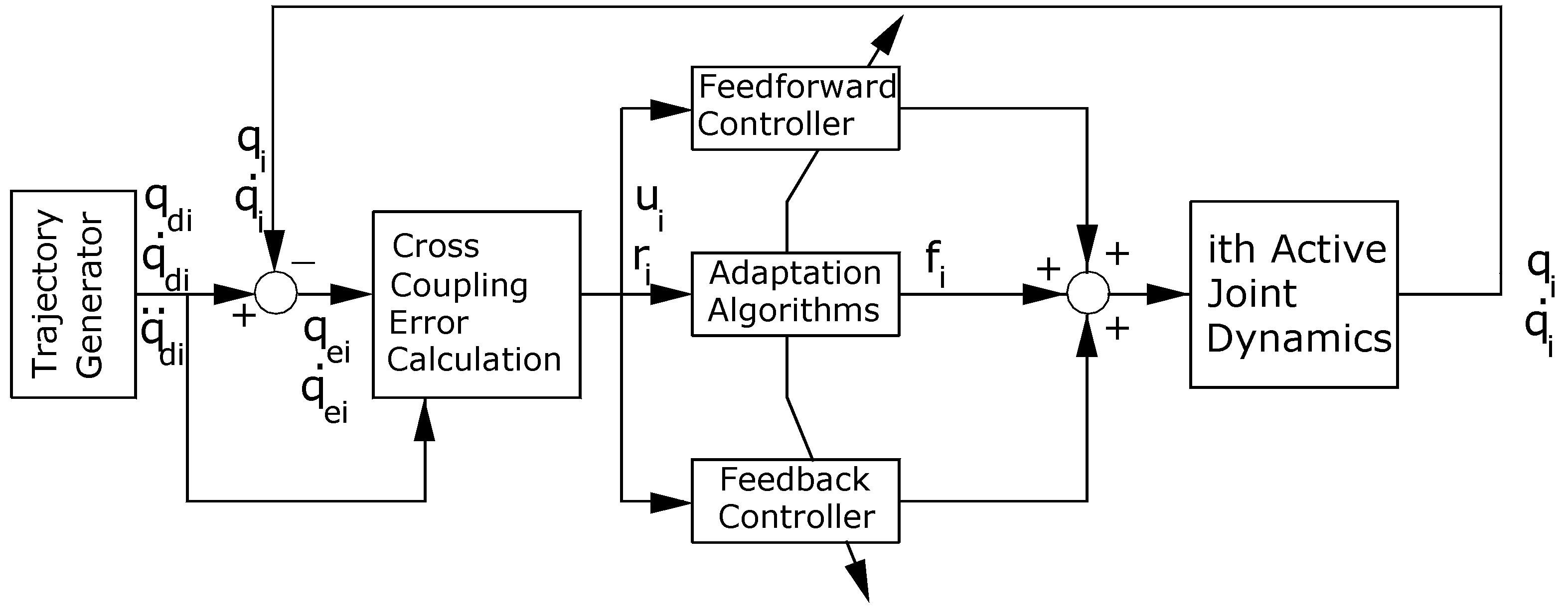
3. Development of the DASCS

The dynamics of a robot manipulator having n active joints can be expressed in joint-space as follows [33]:

$$M\left(q\right)\ddot{q}+N\left(q,\dot{q}\right)+G\left(q\right)+H\left(\dot{q}\right)=T\left(t\right)$$

(9)

where $q$ is the n × 1 vector of joint displacement, $M\left(q\right)$ is the n × n symmetric positive definite inertia matrix, $N\left(q,\dot{q}\right)$ is the n × 1 Coriolis and centrifugal torque vector, $G\left(q\right)$ is the n × 1 gravitational torque vector, and $H\left(\dot{q}\right)$ is the n × 1 frictional torque vector.

The ith subsystem of the dynamical system (9) can be expressed in the following decentralized form [30]:

$$m_{ii}\left(q\right){\ddot{q}}_{ii}\left(t\right)+\left[{\sum }_{\begin{array}{c}j=1\\ j\ne 1\end{array}}^6{m}_{ij}\left(q\right){\ddot{q}}_j\left(t\right)\right]+n_i\left(q,\dot{q}\right)+g_i\left(q\right)+h_i\left(\dot{q}\right)=T_i\left(t\right)$$

(10)

where $T_i$ is the control input of the ith active joint.

As seen in (10), the ith subsystem not only contains the gravity, friction, Coriolis, and centrifugal torque, namely $n_i\left(q,\dot{q}\right)+g_i\left(q\right)+h_i\left(q\right)$ for the ith active joint, but also is coupled between it and the remaining subsystems shown by the term $\left[\sum _{\begin{array}{c}j=1\\ j\ne 1\end{array}}^6{m}_{ij}\left(q\right){\ddot{q}}_j\left(t\right)\right].$

Let

$$d_i\left(q,\dot{q},\ddot{q}\right)={\sum }_{\begin{array}{c}j=1\\ j\ne 1\end{array}}^6{m}_{ij}\left(q\right){\ddot{q}}_j\left(t\right)+n_i\left(q,\dot{q}\right)+g_i\left(q\right)+h_i\left(\dot{q}\right)$$

(11)

Then, (10) becomes the following:

$$m_{ii}\left(q\right){\ddot{q}}_{ii}\left(t\right)+d_i\left(q,\dot{q},\ddot{q}\right)=T_i\left(t\right)$$

(12)

Next, we define a command vector $u_i\left(t\right)$ as follows:

$$u_i\left(t\right)=q_{di}\left(t\right)+\beta {\int }_0^t{[\epsilon }_n\left(w\right)-{\epsilon }_{n-1}\left(w\right)]dw+\alpha {\int }_0^t{e_i}^{*}\left(w\right)dw$$

(13)

where $q_{di}\left(t\right)$ denotes the desired trajectory of the ith active joint and $\alpha$ is a positive constant. We also define a generalized error $r_i\left(t\right)$ as follows [30]:

$$r_i\left(t\right)=u_i\left(t\right)-q_i\left(t\right)={e_i}^{*}\left(t\right)+\alpha {\int }_0^t{e_i}^{*}\left(w\right)dw$$

(14)

Now a control law for the ith subsystem in (10) can be defined as follows:

$$T_i\left(t\right)=f_i\left(t\right)+\left[k_{0i}\left(t\right)r_i\left(t\right)+k_{1i}\left(t\right){\dot{r}}_i\left(t\right)\right]+\left[a_i\left(t\right)u_i\left(t\right)+b_i\left(t\right){\dot{u}}_i\left(t\right)+c_i\left(t\right){\ddot{u}}_i\left(t\right)\right]$$

(15)

Substituting (15) into (10) in light of (12) and dropping the subscript i for simplicity, we obtain the error differential equation in terms of the generalized error r(t), which is indeed $r_i\left(t\right)$as follows:

$$m\ddot{r}\left(t\right)+k_1\left(t\right)\dot{r}\left(t\right)+k_0\left(t\right)r\left(t\right)=d-f\left(t\right)-a\left(t\right)u\left(t\right)-b\left(t\right)\dot{u}\left(t\right)+\left(m-c\right)\ddot{u}\left(t\right)$$

(16)

Let us define the 2 × 1 position-velocity error vector $X\left(t\right)=\left(\begin{array}{c}r\left(t\right)\\ \dot{r}\left(t\right)\end{array}\right)$ and then express Equation (16) in a state space form as follows:

$$\dot{X}\left(t\right)=\left(\begin{array}{cc}0& 1\\ {-∆}_1& -{∆}_2\end{array}\right)X\left(t\right)+\left(\begin{array}{c}0\\ {∆}_0\end{array}\right)+\left(\begin{array}{c}0\\ {∆}_3\end{array}\right)u\left(t\right)+\left(\begin{array}{c}0\\ {∆}_4\end{array}\right)\dot{u}\left(t\right)+\left(\begin{array}{c}0\\ {∆}_5\end{array}\right)\ddot{u}\left(t\right)$$

(17)

where the variables ${∆}_1={\displaystyle \frac{k_0}{m}}$; ${∆}_2={\displaystyle \frac{k_1}{m}}$; ${∆}_0={\displaystyle \frac{d-f}{m}}$; ${∆}_3={\displaystyle \frac{-a}{m}};$ ${∆}_4={\displaystyle \frac{-b}{m}}$; ${∆}_5={\displaystyle \frac{\left(m-c\right)}{m}}$ contain the adjustable controller gains $k_1\left(t\right),k_0\left(t\right),f\left(t\right),a\left(t\right),b\left(t\right),\mathrm{a}\mathrm{n}\mathrm{d} c\left(t\right).$

Equation (17) represents the “adjustable system” in the framework of MRAC. Next, the desired performance of the ith active joint can be specified in terms of a second-order homogeneous differential equation:

$${\ddot{r}}_m\left(t\right)+2\omega \xi {\dot{r}}_m\left(t\right)+{\omega }^2{r}_m\left(t\right)=0$$

(18)

where $\xi$ is the damping ratio, $\omega$ is the natural frequency and $r_m\left(t\right)$ represents the desired trajectory of $r\left(t\right).$

Equation (18) can be written in a state space form as follows:

$${\dot{X}}_m\left(t\right)=\left(\begin{array}{cc}0& 1\\ {-D}_1& -D_2\end{array}\right)X_m\left(t\right)=D{X}_m\left(t\right)$$

(19)

where $D=\left(\begin{array}{cc}0& 1\\ {-D}_1& -D_2\end{array}\right)$, $X_m\left(t\right)=\left(\begin{array}{c}{r}_m\left(t\right)\\ {\dot{r}}_m\left(t\right)\end{array}\right)$, $D_1={\omega }^2$, $D_2=2\omega \xi$ and $r_m\left(t\right)$ and ${\dot{r}}_m\left(t\right)$ are the desired generalized position error and velocity errors, respectively.

Equation (19) represents the “reference model” and its solution is found as follows [30]:

$$X_m\left(t\right)=\exp \left(Dt\right)X_m\left(0\right)$$

(20)

which is under the assumption that the initial values of the actual and the desired trajectory are identical. In other words, $X_m\left(0\right)=0$ yields $X\left(0\right)=0$.

In order for the system to achieve adaptation, we define the adaptation error vector E(t) as follows:

$$E\left(t\right)=X_m\left(t\right)-X\left(t\right)$$

(21)

Then, from (17) and (19), we obtain the following:

$$\dot{E}\left(t\right)=\left(\begin{array}{cc}0& 1\\ {-D}_1& -D_2\end{array}\right)E\left(t\right)+\left(\begin{array}{cc}0& 1\\ {∆}_1{-D}_1& {∆}_1{-D}_1\end{array}\right)X\left(t\right)+\left(\begin{array}{c}0\\ {-∆}_0\end{array}\right)+\left(\begin{array}{c}0\\ {-∆}_3\end{array}\right)u\left(t\right)+\left(\begin{array}{c}0\\ -{∆}_4\end{array}\right)\dot{u}\left(t\right)+\left(\begin{array}{c}0\\ -{∆}_5\end{array}\right)\ddot{u}\left(t\right)$$

(22)

Now, the controller adaptation laws will be derived to achieve the control objective, expressed by $X\left(t\right)⟶X_m\left(t\right)$ or $E\left(t\right)⟶$0 as t$\to$ $\mathrm{\infty }$. To achieve this, we select a Lyapunov function candidate $v\left(t\right)$ [30] such that

$$v\left(t\right)=E^{T}PE+Q_o{\left({\Delta }_0-{{\Delta }_0}^{*}\right)}^2+Q_1{\left({\Delta }_1{-D}_1-{{\Delta }_1}^{*}\right)}^2+Q_2{\left({\Delta }_2{-D}_2-{{\Delta }_2}^{*}\right)}^2+Q_3{\left({\Delta }_3-{{\Delta }_3}^{*}\right)}^2+Q_4{\left({\Delta }_4-{{\Delta }_4}^{*}\right)}^2+Q_5{\left({\Delta }_5-{{\Delta }_5}^{*}\right)}^2$$

(23)

where ${{\Delta }_0}^{*},{{\Delta }_1}^{*},\dots ,{{\Delta }_6}^{*}$ are function of time and $Q_o,Q_1,\dots ,Q_5$ are arbitrary positive scalar.

To stabilize the linear part of (22), it is sufficient to choose ${\xi }_i$ and ${\omega }_i$ such that the matrix D becomes Hurwitz, or all eigenvalues of D have negative real parts. If so, there exists a symmetric positive definite matrix P = $\left[\begin{array}{cc}{P}_1& P_2\\ P_2& P_3\end{array}\right]$ to satisfy the following Lyapunov Equation:

$$PD+D^{T}P=-Q$$

(24)

for any arbitrary symmetric positive definite matrix Q.

Finally, from [30], particularly in the section entitled Derivation of the Adaption Laws, the derivative of $v\left(t\right)$, namely $\dot{v}\left(t\right)$ will be negative definite of $E\left(t\right)$ when we choose the following adaptation laws:

$$\begin{array}{l}f\left(t\right)=f\left(0\right)+{\eta }_2\mathsf{\Omega }\left(t\right)+{\eta }_1{\int }_0^t\mathsf{\Omega }\left(w\right)dw\\ k_0\left(t\right)=k_0\left(0\right)+{\gamma }_2\mathsf{\Omega }\left(t\right)\mathrm{r}\left(t\right)+{\gamma }_1{\int }_0^t\mathsf{\Omega }\left(w\right)\mathrm{r}\left(w\right)dw\\ k_1\left(t\right)=k_1\left(0\right)+{\lambda }_2\mathsf{\Omega }\left(t\right)\dot{r}\left(t\right)+{\lambda }_1{\int }_0^t\mathsf{\Omega }\left(w\right)\dot{r}\left(w\right)dw\\ a\left(t\right)=\mathrm{a}\left(0\right)+{\mu }_2\mathsf{\Omega }\left(t\right)\mathrm{u}\left(t\right)+{\mu }_1{\int }_0^t\mathsf{\Omega }\left(w\right)\mathrm{u}\left(w\right)dw\\ b\left(t\right)=b\left(0\right)+{\rho }_2\mathsf{\Omega }\left(t\right)\dot{u}\left(t\right)+{\rho }_1{\int }_0^t\mathsf{\Omega }\left(w\right)\dot{u}\left(w\right)dw\\ c\left(t\right)=c\left(0\right)+{\sigma }_2\mathsf{\Omega }\left(t\right)\ddot{u}\left(t\right)+{\sigma }_1{\int }_0^t\mathsf{\Omega }\left(w\right)\ddot{u}\left(w\right)dw\end{array}$$

(25)

where ${\eta }_1,{\gamma }_1,{\lambda }_1,{\mu }_1,{\rho }_1,{\sigma }_1$ are positive constant and ${\eta }_2,{\gamma }_2,{\lambda }_2,{\mu }_2,{\rho }_2,{\sigma }_2$ are zero or positive constant, $\mathsf{\Omega }\left(t\right)=P_{2}r\left(t\right)+P_3\dot{r}\left(t\right)$ where $P_2$ and $P_3$ are positive constant, depending on the reference model. Furthermore, $f$(0), $k_0$(0), $k_1$(0), $a$(0), $b\left(0\right)$, $c\left(0\right)$ which are the initial conditions of $f\left(t\right)$, $k_0\left(t\right)$, $k_1\left(t\right)$, $a\left(t\right)$, $b\left(t\right)$,$c\left(t\right)$, respectively, can be set arbitrarily.

As a result, $X\left(t\right)⟶$0 as $t\to$ $\mathrm{\infty }$ results in $\left[\begin{array}{c}{e_i}^{*}\left(t\right)+\beta {\int }_0^t{e_i}^{*}\left(w\right)dw\\ {{\dot{e}}_i}^{*}\left(t\right)+\beta {e_i}^{*}\left(t\right)\end{array}\right]⟶0$ as t$\to$ $\mathrm{\infty }$.

Then, ${e_i}^{*}\left(t\right)⟶0$ and ${{\dot{e}}_i}^{*}\left(t\right)⟶0$ as t$\to$ $\mathrm{\infty }$ [34]. Thus, ${q_{ei}\left(t\right)}_{,}$ ${\dot{q}}_{ei}\left(t\right)$ are bounded from (9) and from differentiating (9). Moreover, ${\dot{\epsilon }}_i\left(t\right)$ are bounded from differentiating (8), then ${\epsilon }_i\left(t\right)$ are uniformly continuous since every function which is differentiable and has bounded derivative is uniformly continuous [35,36].

From Barbalat’s Lemma [36], suppose that $f:\left[0,\mathrm{\infty }\right]\to \mathbb{R}$ is uniformly continuous and its derivative is bounded. Then, $f\left(t\right)⟶0$ as t$\to$ $\mathrm{\infty }$ holds. Therefore, ${\epsilon }_i\left(t\right)⟶0$ as t$\to$ $\mathrm{\infty }$ since ${\epsilon }_i\left(t\right)$ are uniformly continuous and ${\dot{\epsilon }}_i\left(t\right)$ are bounded. From (8) and (9), ${\epsilon }_i\left(t\right)⟶0$ and ${e_i}^{*}\left(t\right)⟶0$ results in $e_i\left(t\right)⟶0$ as t$\to$ $\mathrm{\infty }$ for all $i=1-n$. Therefore, the control objective is achieved.

It is noted that the adaptation laws are solutions for controller gain matrices of control law (15) and based on the actual, desired performances and their derivatives. Furthermore, we note that the control law (15) consists of three terms:

• The first term $f_i\left(t\right)$ represents auxiliary signal to improve the tracking performance and partly compensate for disturbance $d\left(t\right)$.
• The second term ${\tau }_i^{fb}\left(t\right)=\left[k_{0i}\left(t\right)r_i\left(t\right)+k_{1i}\left(t\right){\dot{r}}_i\left(t\right)\right]$=${[k}_{0i}\left(t\right)+\alpha ]{e_i}^{*}\left(t\right)+{\alpha k}_{0i}\left(t\right){\int }_0^t{e_i}^{*}\left(w\right)dw]+k_{1i}\left(t\right)\dot{{e_i}^{*}}\left(t\right)$ represents the PID feedback controller.
• The last term ${\tau }_i^{ff}\left(t\right)=\left[a_i\left(t\right)u_i\left(t\right)+b_i\left(t\right){\dot{u}}_i\left(t\right)+c_i{\ddot{u}}_i\left(t\right)\right]$ represent the feedforward controller.

The structure of the controller is shown in Figure 1. The required inputs of the ith controller are the desired position, velocity, and acceleration of its active joint. The required measurements are the actual positions and velocities of its active joint and the two adjacent ones.

4. Computer Simulation Study of a 6-DOF CKCM Manipulator

This section presents a computer simulation study conducted to evaluate the effectiveness of the developed DASCS applied to control the motion of a 6-DOF CKCM manipulator. A brief kinematic analysis of this manipulator will first be presented, followed by a presentation and discussion of the computer simulation results.

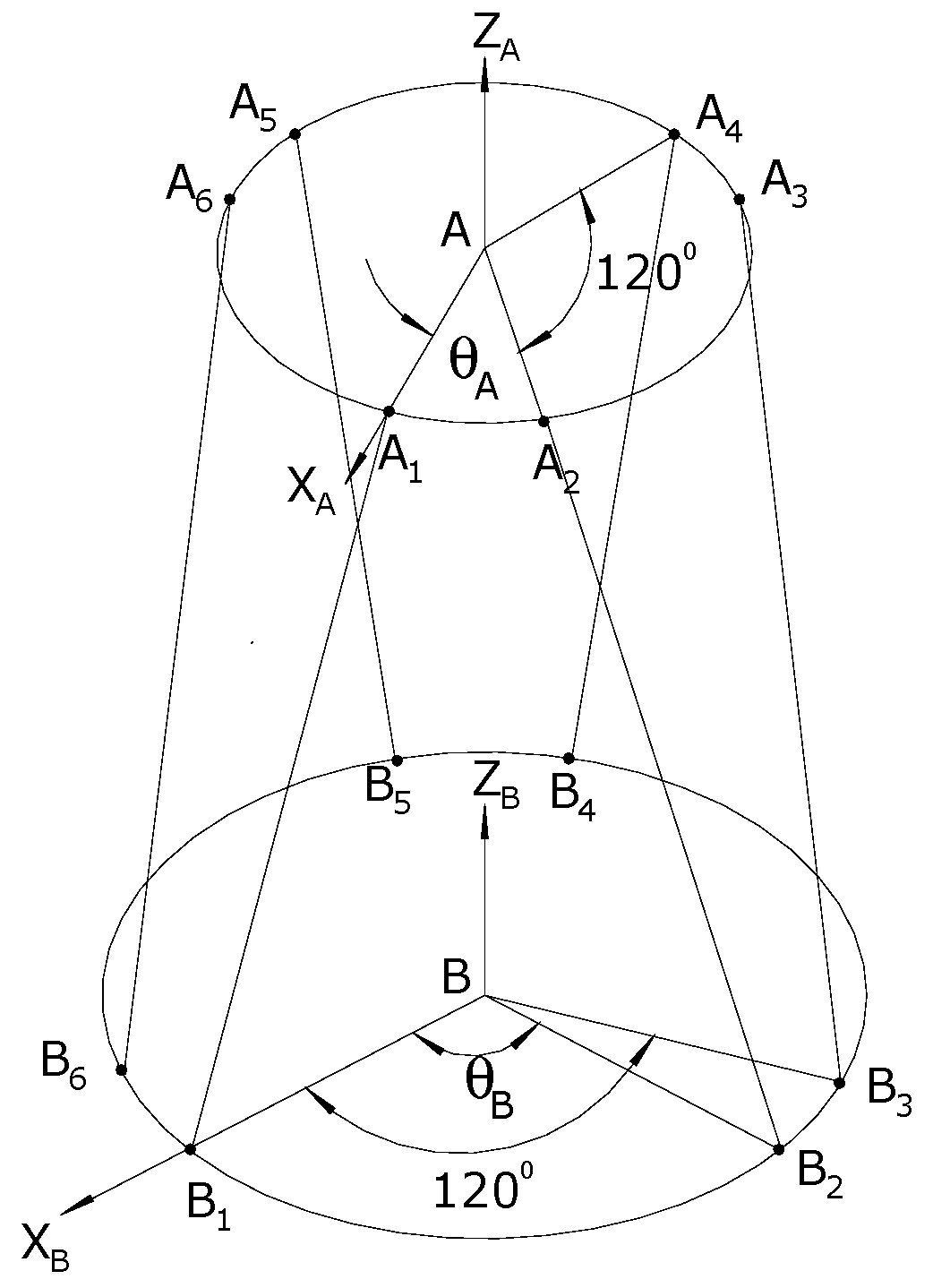
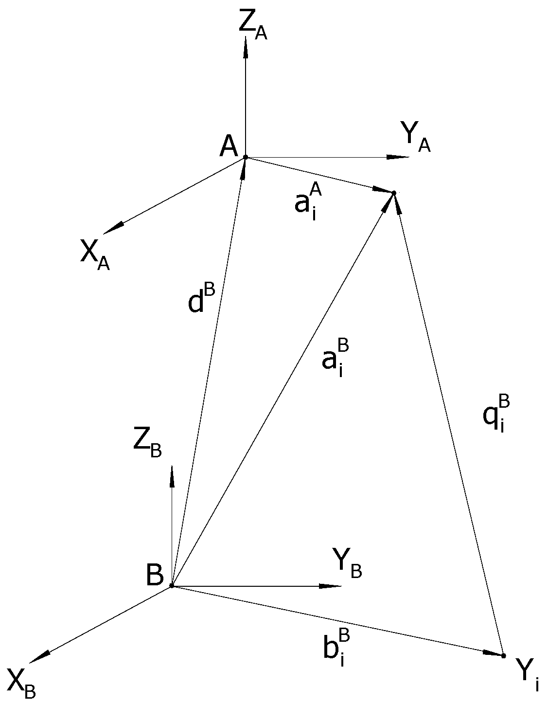
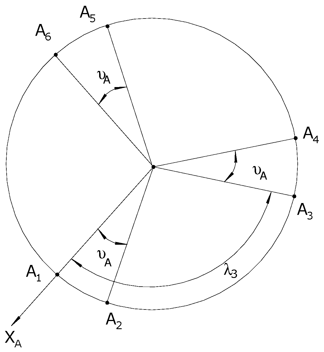
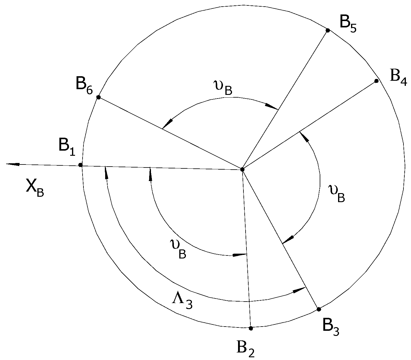
4.1. Kinematic Analysis of the 6-DOF CKCM Manipulator

Figure 2 shows the CKCM manipulator that possesses six DOFs and comprises a stationary base platform and a moving platform coupled together through a number of links. Each link is a linear actuator consisting of a DC motor and a linear ball screw drive and its ends are connected to the base and moving platforms through ball joints.

Figure 3 illustrates the manipulator frame assignment. To represent the position and orientation of the moving platform relative to the base platform, the fixed frame {B} whose origin is at the centroid of the base platform, and the moving frame {A} whose origin is at the centroid of the moving platform are assigned. The assignment of the above coordinate systems complies with the right-hand rule. Points A_i and points B_i are the attachment points of actuator i to the moving platform and base platform, respectively. In addition, each pair of ball joints on the base and moving platform is distributed symmetrically with a separation angle of 120 °C.

Referring to Figure 4, the position vectors ${\mathit{a}}_i^A$, ${\mathit{b}}_i^A$ describe the position of the ball joints at $A_i$, $B_i$ with reference to the moving frame {A} and the stationary base frame {B}, respectively. The radii of the moving and base platforms are denoted by $r_A$ and $r_B$, respectively. In Figure 5, let ${\theta }_A$ represent the angle between ball joints $A_1$ and $A_2$, which is the same between $A_3$ and $A_4$, and $A_5$ and $A_6$. Furthermore, if the angle between ${AA}_i$ and $X_A$-axis is denoted by ${\lambda }_i$ then the position vector ${\mathit{a}}_i^A={\left(a_{ix} a_{iy} a_{iz}\right)}^T$ is computed by the following:

$${\mathit{a}}_i^A={\left[r_A\mathrm{c}\mathrm{o}\mathrm{s}\left({\lambda }_i\right)r_A\mathrm{s}\mathrm{i}\mathrm{n}\left({\lambda }_i\right)0\right]}^T$$

(26)

Similarly, if the angle between ${BB}_i$ and $X_B$-axis is denoted by ${\mathsf{\Lambda }}_i$ as seen in Figure 6, then the position vector ${\mathit{b}}_i^A={\left(b_{ix} b_{iy} b_{iz}\right)}^T$ is given by the following:

$${\mathit{b}}_i^B={\left[r_B\mathrm{c}\mathrm{o}\mathrm{s}\left({\mathsf{\Lambda }}_i\right){ r}_B\mathrm{s}\mathrm{i}\mathrm{n}\left({\mathsf{\Lambda }}_i\right)0\right]}^T$$

(27)

The angles ${\lambda }_i$ and ${\mathsf{\Lambda }}_i$ are determined by the following:

$${\mathsf{\Lambda }}_i=60\left(i-1\right) deg;{\mathsf{\lambda }}_i=60\left(i-1\right)deg, for i=\mathrm{1,3},5$$

(28)

$${\mathsf{\Lambda }}_i={\mathsf{\Lambda }}_{i-1}+{\theta }_B deg;{\mathsf{\lambda }}_i={\mathsf{\lambda }}_{i-1}+{\theta }_{A}deg, for i=\mathrm{2,4},6$$

(29)

The kinematic equations can be derived from the vector diagram for each actuator in Figure 4. The length vector ${\mathit{q}}_i^B={\left(q_{ix} q_{iy} q_{iz}\right)}^T$, expressing the vector $B_i{A}_i$ with respect to frame {B}, can be computed as follows:

$${\mathit{q}}_i^B={\mathit{a}}_i^B-{\mathit{b}}_i^B$$

(30)

where vector ${\mathit{a}}_i^B$ represents the coordinates of point $A_i$ with respect to frame {B}. Vector ${\mathit{d}}_B$ denoting the position of point A with respect to frame {B} is given by the following:

$${\mathit{d}}_B={\left(x y z\right)}^T$$

(31)

where x, y, and z are the Cartesian coordinates of point A in frame {B}. If the orientation of the moving frame {A} with respect to the base frame is specified by Z-Y-X Euler angles $(\alpha \beta \gamma )$, then the corresponding Euler angle orientation matrix ${}_A{}^{B}R$ can be computed as follows:

$${{}_A{}^B\mathit{R}=\mathit{R}}_{zyx,\alpha \beta \gamma }=\left[\begin{array}{ccc}C\alpha C\beta & C\alpha S\beta S\gamma -S\alpha C\gamma & C\alpha S\beta C\gamma +S\alpha S\gamma \\ S\alpha C\beta & S\alpha S\beta S\gamma +C\alpha C\gamma & S\alpha S\beta C\gamma -C\alpha S\gamma \\ -S\beta & C\beta S\gamma & C\beta C\gamma \end{array}\right]$$

(32)

Now vector ${\mathit{a}}_i^B$ can be computed as follows:

$${\mathit{a}}_i^B={}_A{}^B\mathit{R}{a}_i^A+{\mathit{d}}_B$$

(33)

Substituting (33) into (30) yields the following:

$${\mathit{q}}_i^B={}_A{}^B\mathit{R}{\mathit{a}}_i^A+{\mathit{d}}_B-{\mathit{b}}_i^B$$

(34)

Using (34), vector ${\mathit{q}}_i^B$ can be solved for a desired Cartesian configuration of the moving platform, specified by x, y, z, $\alpha \beta \gamma$ as follows:

$${\mathit{q}}_i^B=\left[\begin{array}{c}{q}_{ix}\\ q_{iy}\\ q_{iz}\end{array}\right]=\left[\begin{array}{c}{r}_{11}{a}_{ix}+r_{12}{a}_{iy}+r_{13}{a}_{iz}+x-b_{ix}\\ r_{21}{a}_{ix}+r_{22}{a}_{iy}+r_{23}{a}_{iz}+y-b_{iy}\\ r_{31}{a}_{ix}+r_{32}{a}_{iy}+r_{33}{a}_{iz}+z-b_{iz}\end{array}\right]$$

(35)

where $r_{ij}$ are the elements of the orientation matrix ${}_A{}^B\mathit{R}$ given by (32). After solving for vector ${\mathit{q}}_i^B$, the square of the required corresponding length of the ith actuator, q_i can be computed by the following:

$$q_i^2=\left(q_{ix}^2+q_{iy}^2+q_{iz}^2\right) for i=\mathrm{1,2},\dots ,6$$

(36)

We proceed to substitute (35) into (36) to obtain the following:

$$\begin{array}{l}{q}_i^2=x^2+y^2+z^2+a_{ix}^2+a_{iy}^2+a_{iz}^2+b_{ix}^2+b_{iy}^2+b_{iz}^2\\ +2\left(r_{11}{a}_{ix}+r_{12}{a}_{iy}+r_{13}{a}_{iz}\right)\left(x-b_{ix}\right)\\ +2\left(r_{21}{a}_{ix}+r_{22}{a}_{iy}+r_{23}{a}_{iz}\right)\left(y-b_{iy}\right)\\ +2\left(r_{31}{a}_{ix}+r_{32}{a}_{iy}+r_{33}{a}_{iz}\right)\left(z-b_{iz}\right)-2(x{b}_{ix}+y{b}_{iy}+z{b}_{iz})\end{array}$$

(37)

In Figure 6, since ${\mathit{a}}_i^A$ and ${\mathit{b}}_i^B$ lie on the $x_A-y_A$ plane and $x_B-y_B$ plane, respectively, we have the following:

$$a_{iz}=b_{iz}=0$$

(38)

$$a_{ix}^2+a_{iy}^2+a_{iz}^2=r_A^2$$

(39)

$$b_{ix}^2+b_{iy}^2+b_{iz}^2=r_B^2$$

(40)

Now in light of (39) and (40), (37) becomes the following:

$$\begin{gathered} q_i^2=x^2+y^2+z^2+r_A^2+r_B^2+2\left(r_{11}{a}_{ix}+r_{12}{a}_{iy}\right)\left(x-b_{ix}\right)+2\left(r_{21}{a}_{ix}+r_{22}{a}_{iy}\right)\left(y-b_{iy}\right) \\ +2\left(r_{31}{a}_{ix}+r_{32}{a}_{iy}\right)z-2\left(x{b}_{ix}+y{b}_{iy}\right)for i=1,2,\dots ,6 \end{gathered}$$

(41)

Equation (41) presents the closed-form solution of the inverse kinematics problem, in the sense that the actuator lengths $q_i$ for i = 1, 2…6 can be determined from the Cartesian configuration of the moving platform, specified by x, y, z, $\alpha , \beta , \gamma$.

The forward kinematics of the above six DOF CKCM manipulator deals with the determination of the Cartesian configuration of the moving platform with respect to the base platform, specified by x, y, z, $\alpha \beta \gamma$ based on the actuator lengths, $q_i$ for i = 1, 2…6. Unfortunately, (41) provides six nonlinear simultaneous equations with six unknowns that lead to no closed-form solutions for the forward kinematic problem. As a result, this problem is extremely difficult and needs to be solved by using iterative numerical methods such as the Newton Raphson’s Method [37,38].

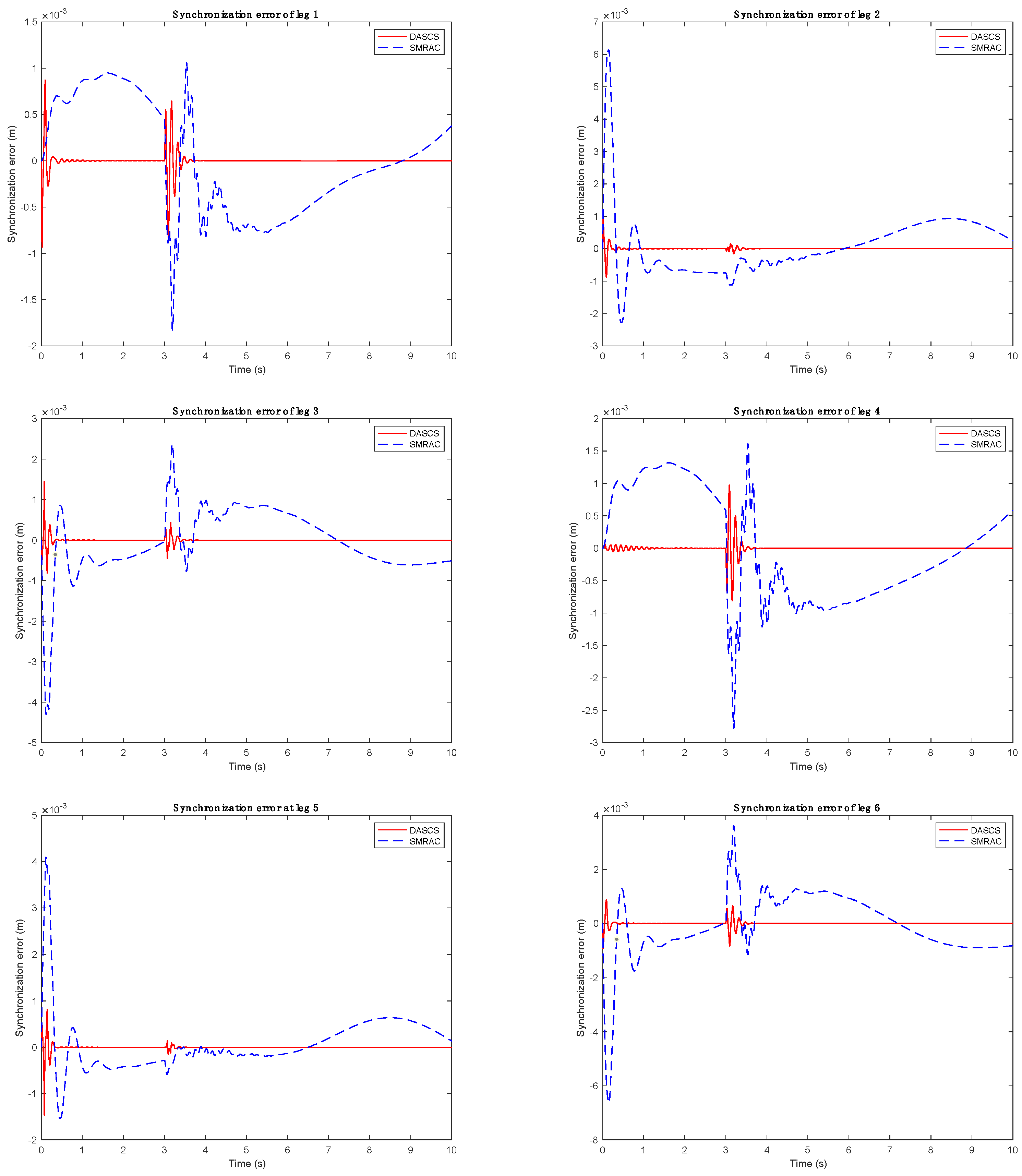
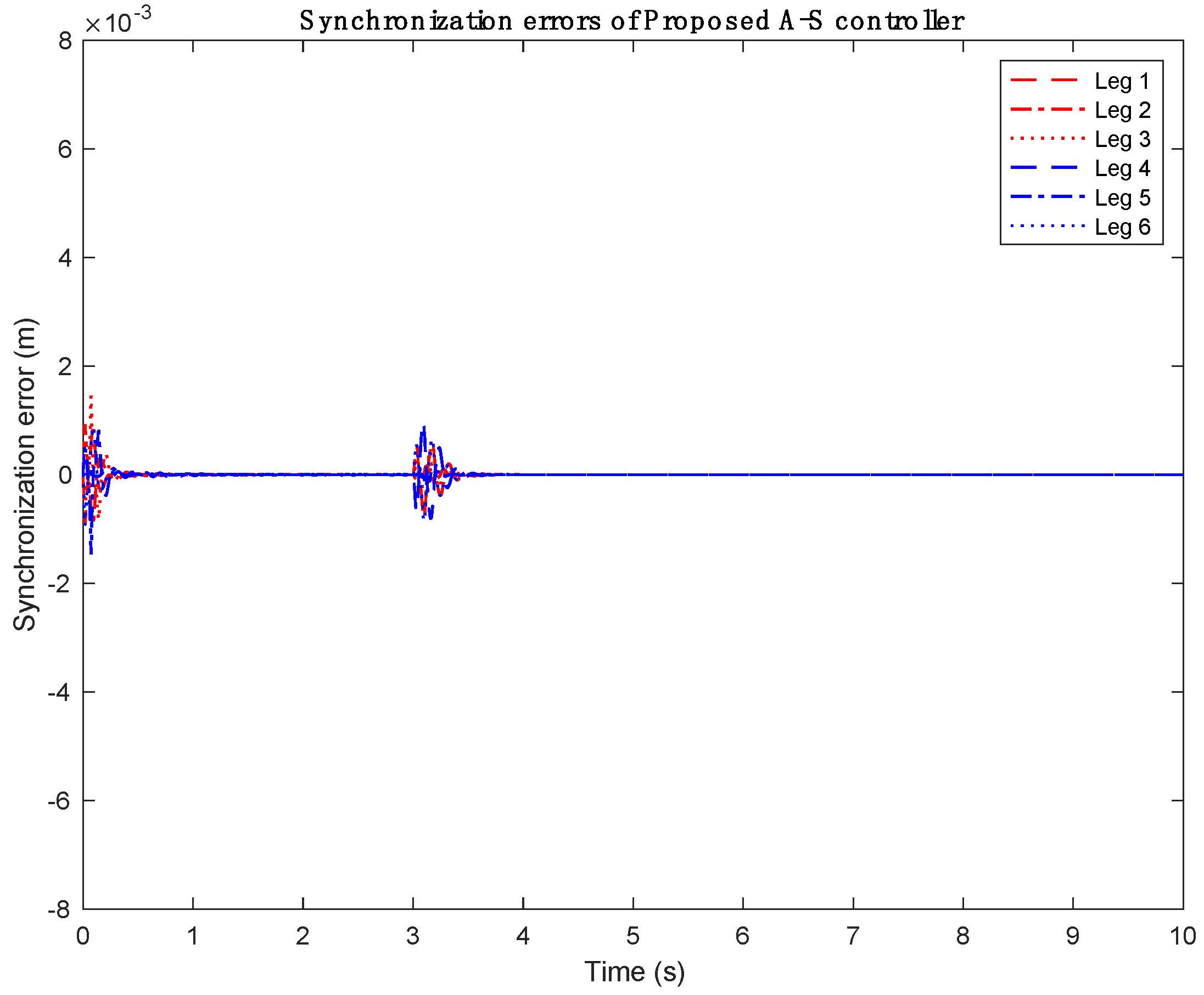
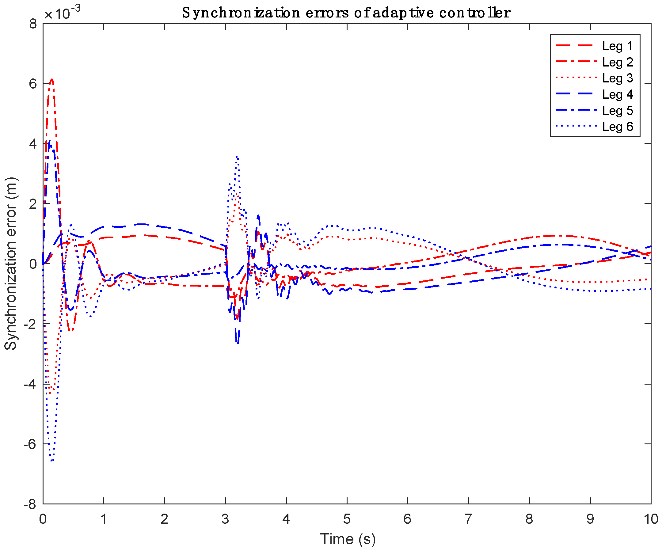
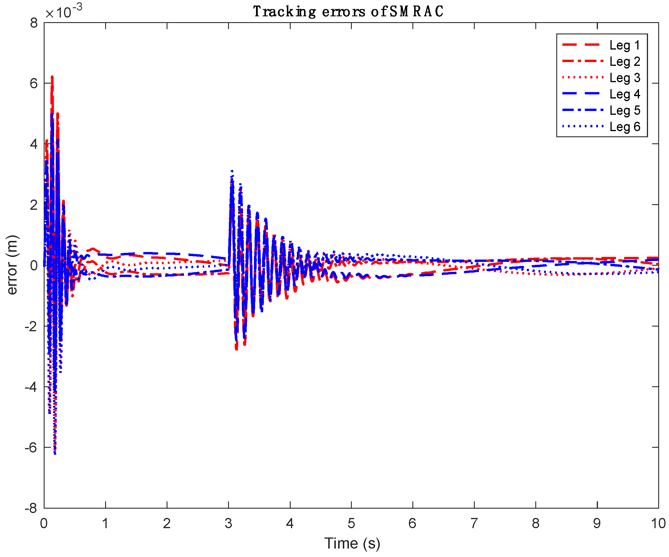
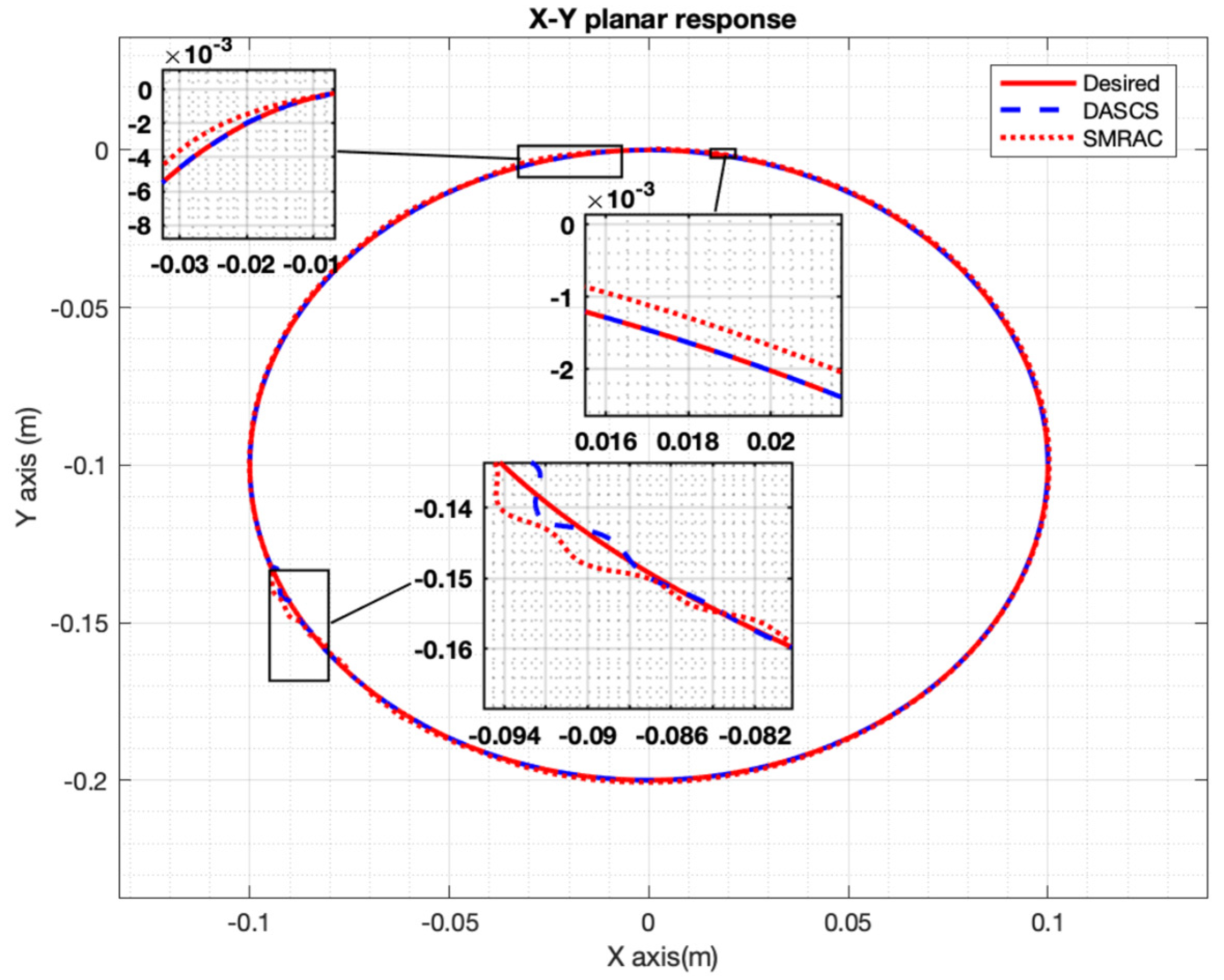
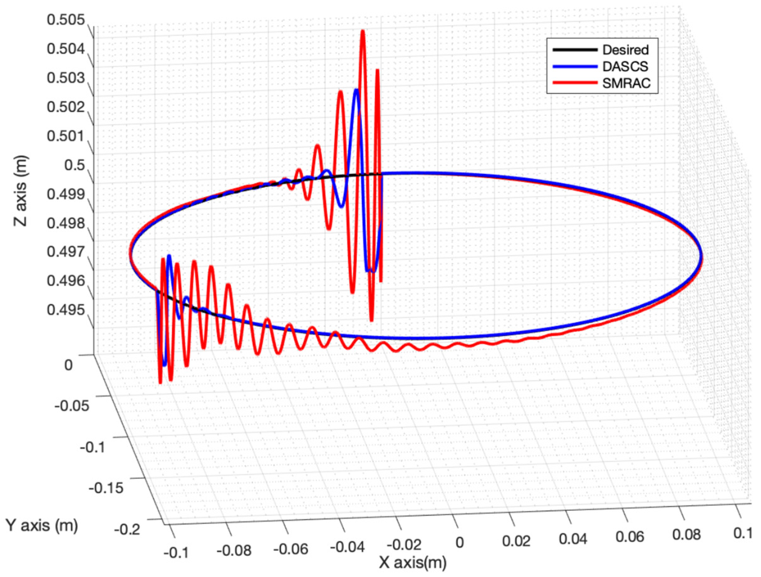
4.2. Computer Simulation Results

Table 1. Parameters of the 6-DOF CKCM manipulator.

Plant Parameters	Value
Base radius (m)	0.36
Platform radius(m)	0.27
Initial height (m)	0.5
Base offset angle (deg)	2.5
Platform offset angle (deg)	10
Mass of the platform (kg)	4.92
Mass of the leg cylinder (kg)	10.29
Inertia coefficient of the platform, Ixx (kg*m2)	0.09
Inertia coefficient of the platform, Iyy (kg*m2)	0.09
Inertia coefficient of the platform, Izz (kg*m2)	0.18

shows the parameters of the above 6 DOF CKCM manipulator employed in the computer simulation study. The computer simulation study is carried out using SimMechanics™, version 2019 which is one of the toolboxes in MATLAB-Simulink, version 19. It provides the ability to easily model and visualize real mechanical systems that consist of multiple rigid bodies. Furthermore, the toolbox takes advantage of the Simulink environment to simulate the physical behaviors and motions of the modelled systems. The SimMechanics library, having the form of interconnected blocks, shows how the physical components with geometric and kinematic relationships of robots are mutually interconnected. Therefore, this approach does not require sophisticated mathematical knowledge about the system to be simulated and presents an easy and precise way to obtain the dynamic model of the system. Figure 7 shows a visualization of the SimMechanics™ model of the manipulator.

For comparison purpose, the developed DASC Scheme (DASCS) and the traditional MRAC scheme (SMRAC) developed by Seraji in [30] were employed to track a reference model with the desired damping ratios and natural frequencies chosen as ${\omega }_i$= 10 rad/s; ${\xi }_i$ = 1, for i = 1, 2, 3, …, 6. We aim to compare the performance of the DASCS with the SMRAC when tracking a circular path in the X-Y plane, described by the following equations:

$$\begin{array}{l}x\left(t\right)=0.1\cos \left(2\pi t\right)\left(\mathrm{m}\right)\\ y\left(t\right)=0.1\sin \left(2\pi t\right)\left(\mathrm{m}\right)\\ z\left(t\right)=0.5\left(\mathrm{m}\right)\end{array}$$

(42)

$$\alpha \left(t\right)=\beta \left(t\right)=\gamma \left(t\right)=0\left(\mathrm{r}\mathrm{a}\mathrm{d}\right)$$

(43)

where $\alpha \left(t\right),\beta \left(t\right),\gamma \left(t\right)$ are rotations about the $x\left(t\right),y\left(t\right),z\left(t\right)$ axes. To evaluate the adaptive ability of the above schemes, a 40 kg payload was suddenly applied at the center of the mass of the moving platform at time t = 3 s.

Figure 8 shows the time trajectories of the synchronization errors of the six legs (actuator lengths, $q_i$ for i = 1, 2…6) for the DASCS and the SMRAC, indicated in red and blue, respectively. As we can see, the synchronization errors of the DASCS are much smaller than those of the SMRAC. As tabulated in

Table 2. Errors for SMRAC and DASCS.

	Maximum Errors		Average Errors
	SMRAC	DASCS	SMRAC	DASCS
$X\left(\mathrm{m}\mathrm{m}\right)$	4.6	0.9602	0.508	0.0226
$Y\left(\mathrm{m}\mathrm{m}\right)$	1.8	1.63	0.501	0.0284
$Z\left(\mathrm{m}\mathrm{m}\right)$	5.1	3.37	0.28	0.0947
$q_{\mathrm{e}1}\left(\mathrm{m}\mathrm{m}\right)$	6.2	3.0340	0.379	0.0988
$q_{\mathrm{e}2}\left(\mathrm{m}\mathrm{m}\right)$	6.1	3.0347	0.323	0.0905
$q_{\mathrm{e}3}\left(\mathrm{m}\mathrm{m}\right)$	6.2	3.3442	0.318	0.0909
$q_{\mathrm{e}4}\left(\mathrm{m}\mathrm{m}\right)$	5	3.2212	0.375	0.0972
$q_{\mathrm{e}5}\left(\mathrm{m}\mathrm{m}\right)$	4.8	2.93	0.331	0.0832
$q_{\mathrm{e}6}\left(\mathrm{m}\mathrm{m}\right)$	6.3	3.3394	0.341	0.0860
${\epsilon }_1\left(\mathrm{m}\mathrm{m}\right)$	1.8325	0.9329	0.5109	0.0021
${\epsilon }_2\left(\mathrm{m}\mathrm{m}\right)$	6.1393	0.9292	0.6637	0.0122
${\epsilon }_3\left(\mathrm{m}\mathrm{m}\right)$	4.3010	1.4477	0.6245	0.0156
${\epsilon }_4\left(\mathrm{m}\mathrm{m}\right)$	2.7799	0.9756	0.7342	0.0176
${\epsilon }_5\left(\mathrm{m}\mathrm{m}\right)$	4.098	1.47	0.3961	0.0117
${\epsilon }_6\left(\mathrm{m}\mathrm{m}\right)$	6.6267	0.9329	0.8946	0.0211

, the average synchronization errors (ASE) of the DASCS are 0.0021 mm, 0.0122 mm, 0.0156 mm, 0.0176 mm, 0.0117 mm, and 0.0211 mm for Leg 1, Leg 2, Leg 3, Leg 4, Leg 5, and Leg 6, respectively, while the ASEs of the SMRAC are 0.5109 mm, 0.6245 mm, 0.7342 mm, 0.3961 mm, 0.54 mm, and 0.8946 mm for Leg 1, Leg 2, Leg 3, Leg 4, Leg 5, and Leg 6, respectively. We also observe that after the introduction of the sudden payload, the DASCS takes 5 s to make the legs converge to their steady states while the SMRAC fails to do so. Moreover, as shown in Figure 9 and Figure 10, the DASC scheme enables the synchronization errors to globally and asymptotically converge to zero while the SMRAC fails to do so. After observing the time trajectories of the synchronization errors of the DASCS and SMRAC in Figure 8, Figure 9 and Figure 10, it is clear that the synchronization errors of the DASCS are “synchronized” while those of the SMRAC are not. This is expected in light of the different characteristics of the two control schemes, with the DASCS having the capability to control the synchronization errors and the SMRAC not having this capability at all.

Figure 11 and Figure 12 show the time trajectories of the tracking errors of the manipulator legs for both control schemes. From the figures, we see that the tracking errors of the DASCS have better transient and steady state responses than those of the SMRAC. As illustrated in Table 2, the average tracking errors (ATE) of the DASCS are 0.0988 mm, 0.0905 mm, 0.988 mm, 0.0909 mm, 0.0972 mm, 0.0832 mm, and 0.0860 mm for Leg 1, Leg 2, Leg 3, Leg 4, Leg 5, and Leg 6, respectively, while the ATEs of the SMRAC are much higher, being 0.379 mm, 0.323 mm, 0.318 mm, 0.375 mm, 0.331 mm, and 0.34 mm for Leg 1, Leg 2, Leg 3, Leg 4, Leg 5, and Leg 6, respectively. In other words, the ATEs of SMRAC are 383%, 356%, 321%, 385%, 397%, and 395% of those of the DASCS. Regarding reaction to the sudden payload change at t = 3 s, the leg time trajectories with the DASCS enter the steady state after $t\ge 3.5 \mathrm{s}$ while those with the SMRAC fail to reach the steady state. Finally, according to the simulation data obtained for the tracking errors, as shown in Table 2, the maximum tracking errors (MTE) for the DASCS are 3.0340 mm, 3.0347 mm, 3.3442 mm, 3.2212 mm, 2.93 mm, and 3.3394 mm for the six actuator legs while the MTEs for the SMRAC are 6.2 mm, 6.1 mm, 6.2 mm, 5 mm, 4.8 mm, and 6.3 mm.

Figure 13 and Figure 14 show the time trajectories of the tracking of the two control schemes in the X-Y plane and the X-Y-Z space, respectively. As the figures show, after the introduction of the sudden payload change, the SMRAC gets off track farther than the DASCS. Moreover, the DASCS has a better ability to track the motion with a much smaller deviation from the desired trajectory until the end of the motion as compared to the SMRAC. We think that the DASCS has a better tracking ability than that of the SMRAC because it employs the configuration error control via the cross-coupling error control.

In conclusion, from the above results of the computer simulation study, overall, the DASCS outperforms the SMRAC when controlling the tracking and synchronization errors due to the fact that the SMRAC only reacts to tracking errors while the DASCS not only reacts to the tracking errors but also to the synchronization errors. In other words, the DASCS controls each active leg to follow its desired trajectory as close as possible while synchronizing its motion with that of other active legs in a defined synchronous manner. We believe that the SMRAC does not effectively react to the sudden change in payload because it lacks the synchronization error control that the DASCS has.

5. Conclusions

This paper considered the problem of motion control of CKCM manipulators because they have several advantages over OKCM manipulators such as higher stiffness, better positioning accuracy, greater payload, and better stability. Solving control problems for CKCMs would result in higher efficiency and productivity of production processes. By treating the trajectory tracking control of a CKCM manipulator as synchronized control of multi OKCM manipulators, we developed a new decentralized adaptive synchronized control scheme, called DASCS, for CKCM manipulators. The development of the DASCS was based on the decentralized concept so that each joint actuator has its own independent controller working with two neighboring ones to achieve the desired motion for the manipulator. In other words, in contrast to conventional decentralized control schemes, each local controller of this new control scheme receives joint position feedback not only from its own joint but also from two neighboring ones. We then applied the model reference adaptive control (MRAC) method based on the Lyapunov direct method into the above synchronized control method to achieve the global asymptotic convergence of tracking errors to zero while synchronizing all active joints’ motions. It is important to note that while conventional MRAC schemes act on joint errors alone, the developed DASCS not only acts on joint errors via synchronization errors but also on cross-coupling errors, which mainly contributes to its enhanced performance as compared to other conventional schemes. Moreover, the developed DASCS, whose controller gains are updated by an adaptation law without the burden of calculating the manipulator dynamics, is computationally efficient and thus is suitable for real-time applications.

To comparatively evaluate the performance of the developed DASCS, we conducted a computer simulation study on a 6-DOF CKCM manipulator whose motions were controlled by the DASCS and a MRAC scheme developed by Seraji [30], namely SMRAC. Simulation results confirmed that the DASCS had better tracking performance for tracking desired motions with and without sudden payload changes as compared to the SMRAC. We concluded that the main reason that the DASCS outperformed the SMRAC was the application of synchronized error control by the DASCS.

Future work on this new control scheme is recommended as follows.

• Experimental investigation of the performance of DASC on real CKCM manipulators in comparison with other conventional MRAC schemes.
• Application of DASCS on OKCM manipulators and evaluation of its performance using computer simulation and experimentation.
• Combination of DASC with other intelligent control methods including fuzzy control, neuro fuzzy control, and neural network control to improve performance.
• Addressing robustness and resilience of synchronized error control of robot manipulators.

References

1. Bi, Z.M.; Lin, Y.; Zhang, W.J. The general architecture of adaptive robotic systems for manufacturing applications. Robot. Comput.-Integr. Manuf. 2010, 26, 461–470. [Google Scholar] [CrossRef]
2. Wu, F.X.; Zhang, W.J.; Li, Q.; Ouyang, P.R. Integrated design and PD control of high-speed closed-loop mechanisms. J. Dyn. Syst. Meas. Control 2002, 124, 522–528. [Google Scholar] [CrossRef]
3. Merlet, J.P. Parallel Robots; Springer Science & Business Media: Berlin/Heidelberg, Germany, 2006; Volume 128. [Google Scholar]
4. Dasgupta, B.; Mruthyunjaya, T.S. The Stewart platform manipulator: A review. Mech. Mach. Theory 2000, 35, 15–40. [Google Scholar] [CrossRef]
5. Stewart, D. A Platform with Six Degrees of Freedom. Proc. Inst. Mech. Eng. 1965, 180, 371–386. [Google Scholar] [CrossRef]
6. Tsai, L.W. Robot Analysis: The Mechanics of Serial and Parallel Manipulators; John Wiley & Sons: Hoboken, NJ, USA, 1999. [Google Scholar]
7. Yanna, Y.; Huiying, W.; Lu, S.; Wei, H. The Influence of Road Geometry on Vehicle Rollover and Skidding. Int. J. Environ. Res. Public Health 2020, 17, 1648. [Google Scholar] [CrossRef]
8. Sun, L.; Zhao, X. Coupled Dynamics of Vehicle-Bridge Interaction System Using High Efficiency Method. Adv. Civ. Eng. 2021, 2021, 1964200. [Google Scholar] [CrossRef]
9. Kelly, R.; Davila, V.S.; Perez, J.A.L. Control of Robot Manipulators in Joint Space; Springer Science & Business Media: Berlin/Heidelberg, Germany, 2006. [Google Scholar]
10. Koren, Y. Cross-coupled biaxial computer control for manufacturing systems. J. Dyn. Syst. Meas. Control 1980, 102, 265–272. [Google Scholar] [CrossRef]
11. Li, Y.; Nielsen, C. Position synchronized path following for a mobile robot and manipulator. In Proceedings of the 52nd IEEE Conference on Decision and Control, Firenze, Italy, 10–13 December 2013; pp. 3541–3546. [Google Scholar]
12. Do, K.D. Synchronization motion tracking control of multiple underactuated ships with collision avoidance. IEEE Trans. Ind. Electron. 2016, 63, 2976–2989. [Google Scholar] [CrossRef]
13. Bouteraa, Y.; Ghommam, J.; Poisson, G.; Derbel, N. Distributed synchronization control to trajectory tracking of multiple robot manipulators. J. Robot. 2011, 2011, 652785. [Google Scholar] [CrossRef]
14. Wang, C.; Sun, D. A synchronization control strategy for multiple robot systems using shape regulation technology. In Proceedings of the 2008 7th World Congress on Intelligent Control and Automation, Chongqing, China, 25–27 June 2008; pp. 467–472. [Google Scholar]
15. Sun, D.; Shao, X.; Feng, G. A model-free cross-coupled control for position synchronization of multi-axis motions: Theory and experiments. IEEE Trans. Control Syst. Technol. 2007, 15, 306–314. [Google Scholar] [CrossRef]
16. Ouyanga, P.R.; Dam, T.; Huang, J.; Zhang, W.J. Contour tracking control in position domain. Mechatronics 2012, 22, 934–944. [Google Scholar] [CrossRef]
17. Shang, W.; Cong, S.; Ge, Y. Coordination motion control in the task space for parallel manipulators with actuation redundancy. IEEE Trans. Autom. Sci. Eng. 2012, 10, 665–673. [Google Scholar] [CrossRef]
18. Sun, D.; Wang, C.; Shang, W.; Feng, G. A synchronization approach to trajectory tracking of multiple mobile robots while maintaining time-varying formations. IEEE Trans. Robot. 2009, 25, 1074–1086. [Google Scholar]
19. Sun, D.; Mills, J.K. Adaptive synchronized control for coordination of two robot manipulators. In Proceedings of the 2002 IEEE International Conference on Robotics and Automation (Cat. No. 02CH37292), Washington, DC, USA, 11–15 May 2002; Cat. No. 02CH37292. Volume 1, pp. 976–981. [Google Scholar]
20. Zhu, W.H. On adaptive synchronization control of coordinated multi robots with flexible/rigid constraints. IEEE Trans. Robot. 2005, 21, 520–552. [Google Scholar]
21. Wang, H. Task-space synchronization of networked robotic systems with uncertain kinematics and dynamics. IEEE Trans. Autom. Control 2013, 58, 3169–3174. [Google Scholar] [CrossRef]
22. Long, Y.; Yang, X.J. Robust adaptive fuzzy sliding mode synchronous control for a planar redundantly actuated parallel manipulator. In Proceedings of the 2012 IEEE International Conference on Robotics and Biomimetics (ROBIO), Guangzhou, China, 11–14 December 2012; pp. 2264–2269. [Google Scholar]
23. Fuh, C.C.; Tsai, H.H.; Huang, C.C.A. fuzzy cross-coupled linear quadratic regulator for improving the contour accuracy of bi-axis machine tools. In Proceedings of the 48h IEEE Conference on Decision and Control (CDC) Held Jointly with 2009 28th Chinese Control Conference, Shanghai, China, 15–18 December 2009; pp. 4156–4161. [Google Scholar]
24. Zhao, D.; Zhu, Q.; Li, N.; Li, S. Neural networked based synchronized control for multiple robotic manipulators. In Proceedings of the10th IEEE International Conference on Control and Automation (ICCA), Hangzhou, China, 12–14 June 2013; pp. 1950–1955. [Google Scholar]
25. Yang, G.; Yao, J. Multilayer neurocontrol of high-order uncertain nonlinear systems with active disturbance rejection. Int. J. Robust Nonlinear Control 2024, 34, 2972–2987. [Google Scholar] [CrossRef]
26. Le, D.K.; Ahn, K.K. Synchronization algorithm for controlling 3-R planar parallel pneumatic artificial muscle robot. In Proceedings of the 2011 11th International Conference on Control, Automation and Systems, Gyeonggi-do, Republic of Korea, 26–29 October 2011; pp. 1588–1593. [Google Scholar]
27. Su, Y.X.; Sun, D.; Ren, L.; Wang, X.; Mills, J.K. Nonlinear PD synchronized control for parallel manipulators. In Proceedings of the 2005 IEEE International Conference on Robotics and Automation, Barcelona, Spain, 18–22 April 2005; pp. 1374–1379. [Google Scholar]
28. Sun, D.; Tong, M.C. A synchronization approach for the minimization of contouring errors of CNC machine tools. IEEE Trans. Autom. Sci. Eng. 2009, 6, 720–729. [Google Scholar]
29. Zhao, D.; Li, S.; Gao, F. Fully adaptive feedforward feedback synchronized tracking control for Stewart Platform systems. Int. J. Control Autom. Syst. 2008, 6, 689–701. [Google Scholar]
30. Seraji, H. Decentralized adaptive control of manipulators: Theory, simulation, and experimentation. IEEE Trans. Robot. Autom. 1989, 5, 183–201. [Google Scholar] [CrossRef]
31. Sun, D.; Mills, J.K. Adaptive Synchronized Control for Coordination of Multirobot Assembly Tasks. IEEE Trans. Robot. Autom. 2002, 18, 498–510. [Google Scholar]
32. Sun, D. Position synchronization of multiple motion axes with adaptive coupling control. Automatic 2003, 39, 997–1005. [Google Scholar] [CrossRef]
33. Craig, J. Robotics: Mechanics and Control; Addison-Wesley: Reading, MA, USA, 1986. [Google Scholar]
34. Slotine, J.J.E.; Li, W. On the adaptive control of robot manipulators. Int. J. Robot. Res. 1987, 6, 49–59. [Google Scholar] [CrossRef]
35. O’Searcoid, M. Metric Spaces; Springer Science & Business Media: Berlin/Heidelberg, Germany, 2006. [Google Scholar]
36. Khalil, H.K.; Grizzle, J.W. Nonlinear Systems; Prentice Hall: Upper Saddle River, NJ, USA, 2002; Volume 3. [Google Scholar]
37. Nguyen, C.C.; Zhou, Z.; Antrazi, S.S.; Campbell, C.E. Efficient computation of forward kinematics and Jacobian matrix of a Stewart platform-based manipulator. In Proceedings of the IEEE Proceedings of the SOUTHEASTCON ′91, Williamsburg, VA, USA, 7–10 April 1991; Volume 2, pp. 869–874. [Google Scholar]
38. Merlet, J.P. Solving the forward kinematics of a Gough-type parallel manipulator with interval analysis. Int. J. Robot. Res. 2004, 23, 221–235. [Google Scholar] [CrossRef]
Figure 1. Decentralized adaptive synchronized control scheme of the ith active joint.
Machines 13 00331 g001
Figure 2. The six DOF CKCM manipulator.
Machines 13 00331 g002
Figure 3. Frame assignment for the CKCM manipulator.
Machines 13 00331 g003
Figure 4. Vector diagram for the ith actuator.
Machines 13 00331 g004
Figure 5. Position of the ball joints A i with respect to the X A -axis.
Machines 13 00331 g005
Figure 6. Position of the ball joints B i with respect to the X B -axis.
Machines 13 00331 g006
Figure 7. Simulink model of the 6-DOF CKCM.
Machines 13 00331 g007
Figure 8. Time responses of synchronization errors for SMRAC and DASCS.
Machines 13 00331 g008
Figure 9. Synchronization errors of DASCS.
Machines 13 00331 g009
Figure 10. Synchronization errors of the SMRAC.
Machines 13 00331 g010
Figure 11. Tracking error of the DASCS.
Machines 13 00331 g011
Figure 12. Tracking errors of the SMRAC.
Machines 13 00331 g012
Figure 13. Motion tracking in X-Y plane.
Machines 13 00331 g013
Figure 14. Motion tracking in 3-D (X-Y-Z).
Machines 13 00331 g014