Performance Gain of Collaborative Versus Sequential Motion in Modular Robotic Manipulators for Pick-and-Place Operations

Abstract

With the increasing demand for efficiency and profitability in industrial applications, modularity offers significant advantages such as system reconfiguration, reduced acquisition costs, and enhanced versatility. However, achieving compatibility across multi-vendor modular systems remains a challenge, particularly in motion control. This study focuses on improving motion control and sensing compatibility and performance, partly using open-source tools to enhance performance in modular systems. In such systems, effective motion coordination between modules is crucial; without it, operations are constrained to sequential execution, limiting efficiency. This paper quantifies the performance benefits of collaborative motion compared to sequential motion in modular mechatronic systems for pick-and-place operations. The experimental validation, conducted on a robotic manipulator mounted on a linearly sliding platform, demonstrates a substantial improvement. The results show time savings of 36% to 52% and an approximate 35% reduction in energy consumption, highlighting the potential for improved productivity and sustainability in modular automation solutions.

1. Introduction

As industry is now in its fourth revolution, boosting the productivity and flexibility of industrial processes is essential for manufacturing companies to maintain or increase their market competitiveness [1]. Modular systems have the potential to bring such flexibility and productivity increases. Modularity is defined by the separation of a system into individually replaceable components. Modular systems are therefore less expensive to repair and are inherently flexible by nature. Additionally, the system versatility increases, as swapping certain modules can enable different functionalities [2]. Module sharing between systems can reduce acquisition costs for system operators [2]. Quick system reconfiguration is important in certain manufacturing domains and is enabled by system modularity. This is especially true in the pharmaceutical industry, where the demand for certain products may increase sharply due to epidemic episodes [3,4]. Modular systems can be assembled as multi-vendor systems, meaning compatibility issues must be addressed. Modules ought to be compatible mechanically but their interfaces and control algorithms should integrate and function together [2,5]. Two recent studies focused on the compatibility of mechatronic modular systems [6,7]; both developed frameworks to ensure compatibility in the design of modules. In [8], an algorithm was developed in Matlab for rapid design of modular serial robotics. In non-modular systems, centralized control algorithms are commonly used. However, in multi-vendor modular systems, compatibility can be challenging or even impossible due to vendor-specific communication protocols, software, and mechanical interfaces. Furthermore, in certain applications, safety regulations may also restrict the simultaneous operation of modules [2]. Sequential operation is then used, unfortunately increasing system execution time and thus reducing system efficiency and profitability. Development of integrated software solutions is a complex and time-consuming task. With sequential operation of module actions, the necessary level of integration is much lower than with coordinated simultaneous motion. System designers and operators must therefore make application-specific decisions on the needed level of integration.

Current research on evaluating the impact of modularity in the manufacturing industry is limited to supply chain studies, product modularity, and assembly line use-case studies. In [9], a modular production of small-scale ships shows a specific time reduction of a factor of $1.5$ and a cost reduction of a factor of 4. A new methodology for the optimal planning of modular automotive assembly lines is developed and applied to a practical use case in [10], highlighting its improved flexibility and adaptability. Modular supply chains and product families were shown to be economically advantageous compared to non-modular ones in [11]. Modularity has also been studied at the control level, with a modular distributed control algorithm developed for multiple robots operating together in [12]. A modular manufacturing process simulation environment was used to simulate reconfiguration of a modular manufacturing environment, resulting in a 10% time saving compared to a non-reconfigurable case [13].

Robotic manipulators and their advantages have also been studied in the literature. In [14], it is shown that small and medium enterprises could benefit from an up to 8% capacity increase by employing robotic manipulators for pick-and-place operations. The time to market for developing modular service robots, a type of modular robot, was estimated to be 30% to 40% lower compared to non-modular service robots in [2]. This study also indicated a 15% lower acquisition cost for modular service robots due to component sharing. Extensive research has been conducted on path planning and control of mobile robotic manipulators, such as in [15,16,17]. An LQR (linear–quadratic regulator) control scheme is developed for four-wheeled mobile robots in [15]; the control scheme is shown to outperform traditional PID (proportional–integral–derivative) controllers. A friction-based feedforward controller is implemented on a modular mechatronic robot in [18]. The interference between multiple actuators is handled by a third-order active disturbance rejection controller in [19]. In [20], an adaptive model-based sliding mode controller is proposed for an unmanned ground vehicle. It is shown to maintain performance under nonlinear disturbances and un-modeled dynamics. Notwithstanding the improved tracking control performance of the two controllers developed in the previously cited papers, the actuator control used in the present study is PID-based due to its current industry relevance, simple tuning, and adequate performance under known operating conditions. In [16], a neural network-based path planner is developed and proposed for a high-DOF (degrees of freedom) robot. In [17], a rapidly exploring random tree algorithm is used for path planning of an agricultural mobile robot. An A* algorithm (graph traversal and path finder) was used on a collaborative robot in [21]. In this paper, an optimization-based trajectory planner was used with the goal of limiting tuning costs: a wide range of engineering specifications can be straightforwardly mapped into constraints and objectives with physical interpretations. This comes with higher computational costs than the aforementioned methods.

The estimation of task execution time is essential in factory planning and assembly line balancing. Robot vendors propose costly and brand-specific software for this purpose. A lower-cost alternative was developed in [22]. Specifically, a mathematical description of the task sequence is used in conjunction with robot-specific dynamic constraints to generate optimal trajectories. The task execution time is estimated from these trajectories and is shown to be close to the estimates from the robot vendors’ software. Cooperation in robotics can occur in the form of two modules of a single system or two independent systems cooperating. In [23], a dual-arm robot reduced task execution time by 20% compared to a single-arm robot, which was attributed to collaboration of the two arms. Idle and active times of human–robot collaboration were studied in [24], showing potential for planning optimization; much like when two modules move collaboratively. In [25,26], human–robot cooperation was shown to improve assembly (similar to pick-and-place) operations by at least 10%. Refs. [27,28] found an 86% time saving when using human–robot collaboration for a series of pick-and-place tasks. In [29], human–robot cooperation was studied for an assembly operation while varying the percentage of time spent cooperating. They linked the productivity gains to the degree of collaboration, task allocation fraction, and operation complexity. While human–robot collaboration has been widely studied, research on cooperation between robots remains limited despite its potential for similar efficiency gains.

In the present paper, the virtual commissioning framework developed in [30] is used to estimate execution times for predefined task sequences. However, the focus is on comparing the estimated times for collaborative and sequential motion. Collaborative mode is defined in this paper as the simultaneous transient and steady-state motion of two mechatronic modules. Conversely, sequential mode is defined as transient and steady-state motion of one module while the other module is in standstill or in steady-state motion.

While there is a considerable number of research papers addressing modularity in industrial robotics, research is lacking on the quantification of time savings obtained with modular systems for pick-and-place operations. There exist some economic viability studies on certain topics, as mentioned in the literature study above, but the performance advantages of collaborative motion in modular manipulator systems for pick-and-place operations have not been thoroughly studied. It is intuitively clear that this collaborative movement of modular manipulators enhances efficiency and profitability. The quantification of time and energy benefits in modular mechatronic systems remains largely unexplored and highly application dependent. This paper addresses this research gap by presenting simulations and experimental analyses of time and energy savings obtained through collaborative motion compared to sequential motion for pick-and-place operations. Concretely, the contributions of this study are as follows:

• The potential time gain when using collaborative motion compared to sequential motion is quantified using realistic multi-body motion simulations.
• Experimental validation of this time gain is provided on a linear track + 6-DOF robotic arm system with a pick-and-place use case.
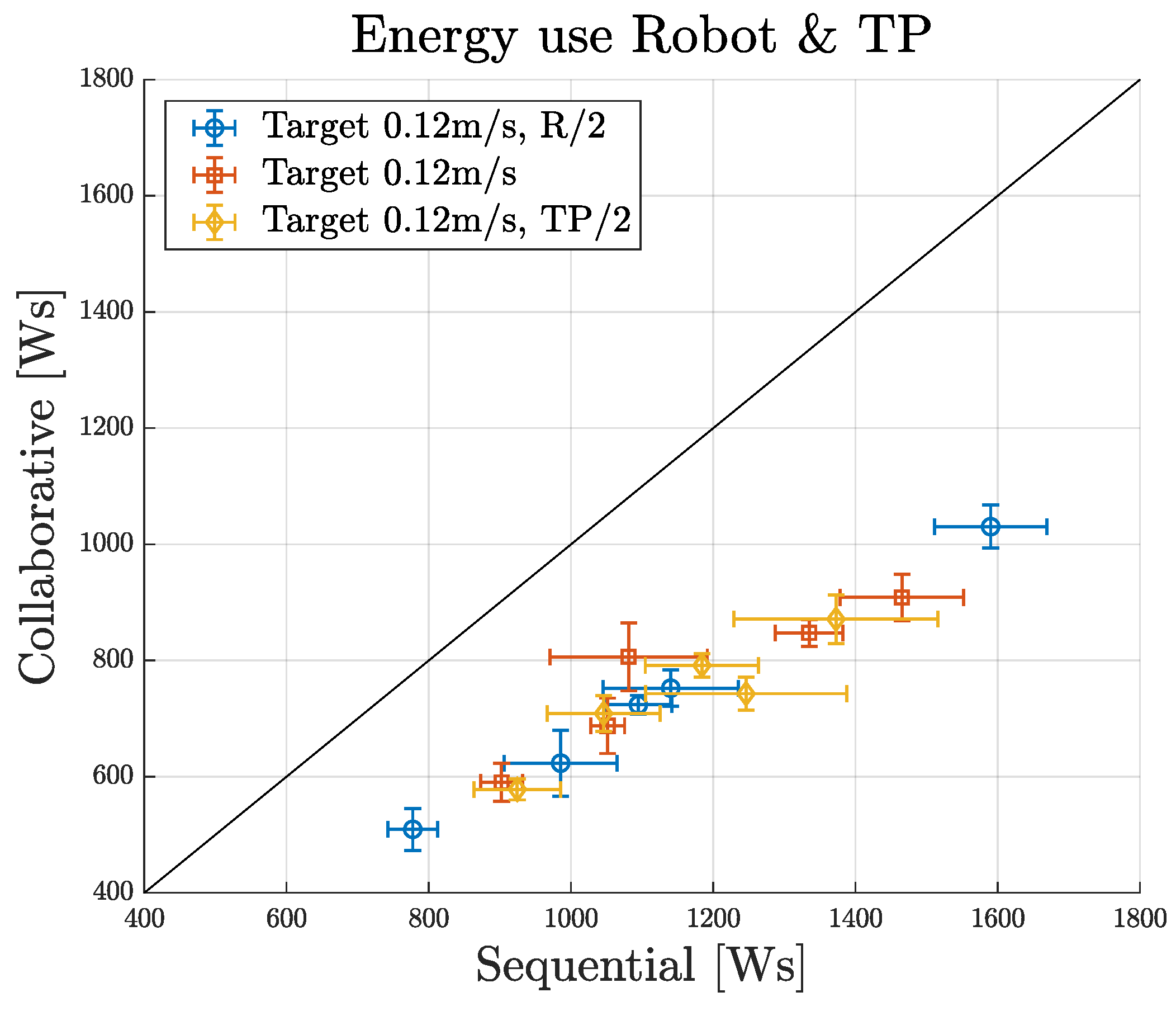
• The corresponding gain in energy savings is quantified and validated.
• A software architecture for control and perception is presented, based on open-source components, which enables collaborative motion in modular mechatronic systems.

These analyses are targeted at industry professionals, providing clear guidelines for design, configuration, and operation decisions, motivated by a quantification of the potential performance gain in the form of time and energy.

This paper is structured as follows: the control and sensing algorithms are described in Section 2. The simulation model and experimental setup are described in Section 3; the simulation and experimental test cases are defined in Section 4; and the results are presented and discussed in Section 5.

2. Control and Sensing Architecture

This section provides a brief overview of the world model. Subsequently, it describes the two main levels of control software shown in Figure 1, including their objectives, operating mechanisms, and structure.

2.1. World Model

Planning and control modules require knowledge of the physical environment to identify key points that enable the avoidance of collisions with static and dynamic obstacles. Static objects can be mapped beforehand, while moving or unknown objects must be monitored in real time using perception sensors like cameras. The world model fuses data from multiple sensors and combines them with model-based predictions and/or prior information to create a structured, semantic representation of the environment. Examples of these various sensors are cameras, lidars, encoders, etc. In addition to sensor fusion, the world model functions as a database, providing relevant environmental data to planning and control modules. It provides services to query obstacles by class, location, or predicted future positions, supporting constraint-aware planning.

2.2. Optimal Trajectory Planner

Once a global task is selected through the GUI (graphical user interface), the task controller, using a Petri net, sends sub-tasks to the Optimal Trajectory Planner (OTP). For each sub-task, a nonlinear optimal control problem (OCP) is solved. The OCP planning horizon starts at a future time, when the solution is expected to have been computed, and extends an unknown length T beyond this. The OCP has the planning horizon time T as its objective and is subject to the following parametric constraints:

• The combined kinematic model of the top sliding platform and robot arm;
• Position, velocity, acceleration, and jerk limits of the top platform and robot joints;
• Collision avoidance based on capsule–capsule distances;
• A boundary constraint for the initial configuration q and its derivative of the robot and top platform;
• Boundary constraints of all joint accelerations and jerks being zero at the start and end of the planning horizon.

When the sub-task involves aligning the robot gripper with a (moving) target, the planner queries the world model for the robot gripper’s current position $d\left(t\right)$ and velocity $\dot{d}\left(t\right)$, assumed to define a steady state. In this case, the following constraint is added to the OCP:

6.

Boundary constraint matching the target’s extrapolated position and orientation with that of the gripper at the end of the planning horizon.

Each possible sub-task has an OCP parametric evaluation function constructed offline through the open-source programs Rockit [31] and CasADi [32]. CasADi is an open-source tool for nonlinear optimization and algorithmic differentiation. It facilitates rapid implementation of different methods for numerical optimal control, both in an offline context and for nonlinear model predictive control (NMPC). Rockit (Rapid Optimal Control Kit) is a software framework to quickly prototype optimal control problems. CasADi version 3.6.3 and Rockit ’workdrive13branch’ were used in this study. The robot joint and top platform trajectories are computed as $4\mathrm{th}$-order B-splines, with their coefficients being the decision variables for the nonlinear program. The system dynamics are indirectly handled by the OCP through the user-defined acceleration and jerk limits. The method could easily be extended to include torque limits based on inverse dynamics if such information was available. The planner queries the world model for obstacles before every sub-task. Signed distances w between robot links and the obstacles are computed and summarized into a single scalar path constraint using the LogSumExp function [33]. For every sub-task, the nonlinear program is solved by IPOPT [34]. This last step is the source of the varying planning time duration depending on randomized initialization for the gradient descent. The computation time is also dependent to a certain degree on the overall cpu load. Practically, the end-user must adjust the position, velocity, acceleration, and jerk constraints to avoid kinematically unfeasible problems or trajectories outside of the actuator and low-level controller bandwidth and limits.

2.3. Low-Level Controller

The low-level controller uses a PID-based cascaded position and speed feedback control loop with feedforward actions. Each degree of freedom has its own independent controller. The low-level controller outputs the desired motor torques ${\mathbf{T}}_{\mathbf{SP}}$ to the drives, which convert them to the required motor current using field-oriented control. The current controllers are auto-tuned by the drives during system configuration. Figure 1 graphically presents the cascaded controller. The control parameters, i.e., the proportional action gains, integral action time constants, and feedforward gains, are tuned in the time domain for minimum tracking root mean squared error (RMSE), minimum settling time, and a constraint on overshoot on spline-shaped trajectories. Specifically, the speed controller’s proportional gain and integral action are tuned for minimum settling time, with an overshoot of around 15% allowed. The position controller gain and feedforward gain are tuned for minimum settling time, with no overshoot allowed. Each joint is tuned in its highest inertia position to ensure stability in all operating points. During operation, each controller receives filtered joint speed $\mathbf{\Omega }$ and position $\mathbf{\Theta }$ feedback data. The planner sends timestamped trajectories as position setpoints ${\mathbf{\Theta }}_{\mathbf{SP}}$ and speed feedforwards ${\mathbf{\Omega }}_{\mathbf{FF}}$. Both the position and speed controller outputs have speed and torque saturation limits in accordance with the mechanical limits of the motor and gearbox.

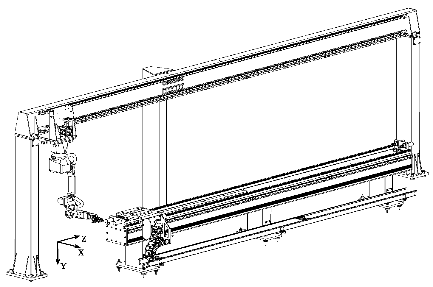
3. Setup Description

Industrial robotic arms can perform a variety of actions but have limited reach. Mounting them on a mobile base or linear track system extends their range of motion, and thus augments their versatility. The test setup employed in this study is designed to mimic an industrial assembly line, i.e., a sliding robotic arm interacting with moving target objects. Figure 2 shows a CAD (computer-aided design) representation of the test setup. The robotic arm is a 6-DOF serial industrial robot rigidly attached to a sliding platform. Below is a second sliding platform on which the target objects are placed. This bottom sliding platform is considered part of the environment.

3.1. Simulation Model

At the heart of the simulation model is a CAD-based co-simulation [30]. The Simcenter solver in Siemens NX models the multi-body dynamics. The NX model is compiled into a Simulink block. This block is parameterized to take joint torque setpoints as inputs. The outputs are the emulated encoder data streams; i.e., joint position and velocity feedback. In Simulink, the joint torque, velocity, and position are constrained according to both motor specifications and the robot’s mechanical limits, maintaining consistency across the entire system. The inertial parameters of each link and the friction characteristics of each joint are individually tuned within the NX model, ensuring realistic values that respect the mechanical limits of both the motors and the robot arm.

Table 1. Motor and mechanical limits of the robot arm. TP = top platform.

DOF	Gearbox Ratio	Max Torque [N m]	Max Speed [°/s]
Robot	118	$35.3$	230
	135	$35.3$	225
	131	$9.14$	230
	14	$4.18$	430
	54	$2.68$	430
	41	$2.68$	630
	Gearbox Ratio	Max Torque [N m]	Max Speed [m/s]
TP	$6.75$	$29.3$	$2.0$

presents the mechanical limits, specifications, and maximum motor torques for each joint.

The simulation model operates on a single computer hosting two virtual machines (VMs) running the various software components. As is shown in Figure 1, a Windows VM runs the NX-Simulink co-simulation while an Ubuntu VM runs Docker containers with the optimal path planner, the task controller, the world model, and the web GUI. With the two VMs forced onto the same IP range, communication between software components occurs through ROS2, as represented by the pink lines and arrows in Figure 1. All software components are synchronized with a combination of the Unix timestamp and the internal simulation time. The simulation runs at a fixed timestep of $200 \mathrm{\mu }\mathrm{s}$.

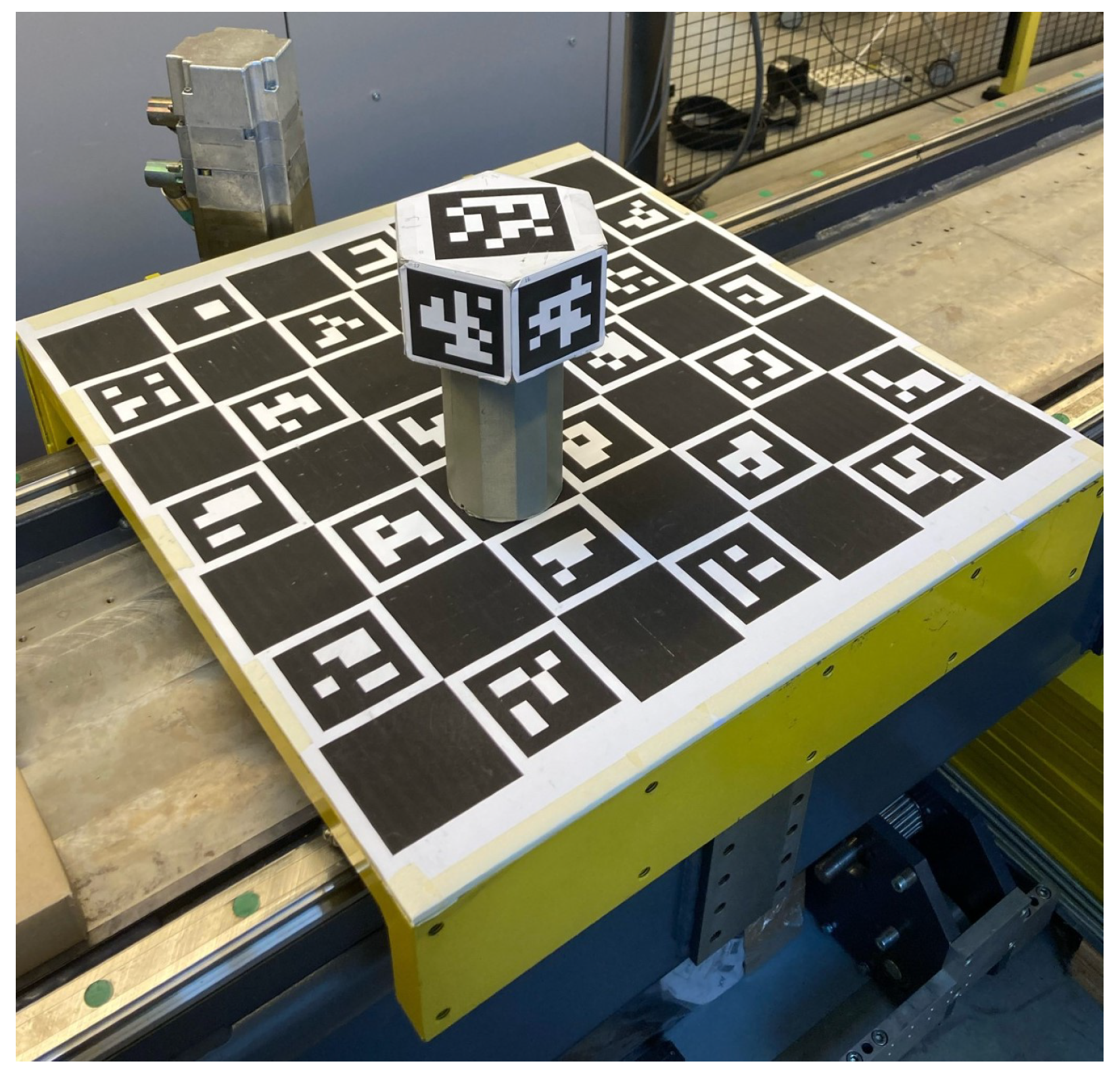
3.2. Experimental Setup

The robot joints and sliding platforms are actuated by position-controlled permanent magnet synchronous motors (PMSMs). The two sliding platforms are driven through a rack-and-pinion mechanism. The bottom sliding platform is considered part of the environment, and is controlled by a separate electrical drive disconnected from the local network. Ceiling-mounted cameras relay the position of the bottom sliding platform to the manipulator system control. The bottom sliding platform has dimensions $0.58 \mathrm{m}$ × $0.63 \mathrm{m}$. The target object to be picked has a height of $0.21 \mathrm{m}$, a bottom cylinder diameter of $0.08 \mathrm{m}$, and a top hexagonal piece with the longest diagonal $0.14 \mathrm{m}$. Figure 3 shows the sliding top platform with the robotic arm and its gripper. Figure 4 shows the Aruco markers used to track both the bottom sliding platform and the target object. The top and bottom sliding platforms can travel, respectively, $7 \mathrm{m}$ and $5 \mathrm{m}$. They are limited to speeds of, respectively, $1.50 \mathrm{m}/\mathrm{s}$ and $0.50 \mathrm{m}/\mathrm{s}$. The robot arm has a reach of $1.42 \mathrm{m}$.

The software scheme of the experimental setup is similar to that of the simulation but with key differences. Compared to Figure 1, the Ubuntu virtual machine is replaced by a real computer running the Docker containers (world model, optimal path planner, task controller, and the GUI). Additionally, the co-simulation environment is replaced with the physical system and the TwinCAT environment running on a Beckhoff CX2043 industrial computer (iPC). The TwinCAT environment hosts the low-level controller along with the electrical drives. The TwinCAT industrial computer communicates with the Ubuntu computer through MQTT over TCP/IP. ROS2 communication is used inside the Ubuntu environment and conversions are handled by an MQTT-ROS2 bridge. All MQTT and ROS2 messages are timestamped using Unix time. The industrial computer and Ubuntu computer are periodically synchronized (every hour) using the Network Time Protocol (NTP). The same NTP server is used for both the Ubuntu computer and the Beckhoff iPC. The low-level controllers are coded in Simulink, then compiled into C++ code (as a TcCOM object). The controllers run as a PLC task with a sample time of $t_s=250 \mathrm{\mu }\mathrm{s}$. The timestamps associated with each passing message allow communication latencies to have minimal impact on operations. For example, the planner accounts for planning time when computing a trajectory; over-estimating this time slightly, by $500 \mathrm{m}\mathrm{s}$, accounts for a high-latency occurrence. In the event that the latency is greater than this value, a very slight jump in position would be observed due to the smooth spline-shaped trajectories. A safety feature is implemented in the low-level controller to guard against larger position jumps that would be caused by a very large (more than $1 \mathrm{s}$) communication delay.

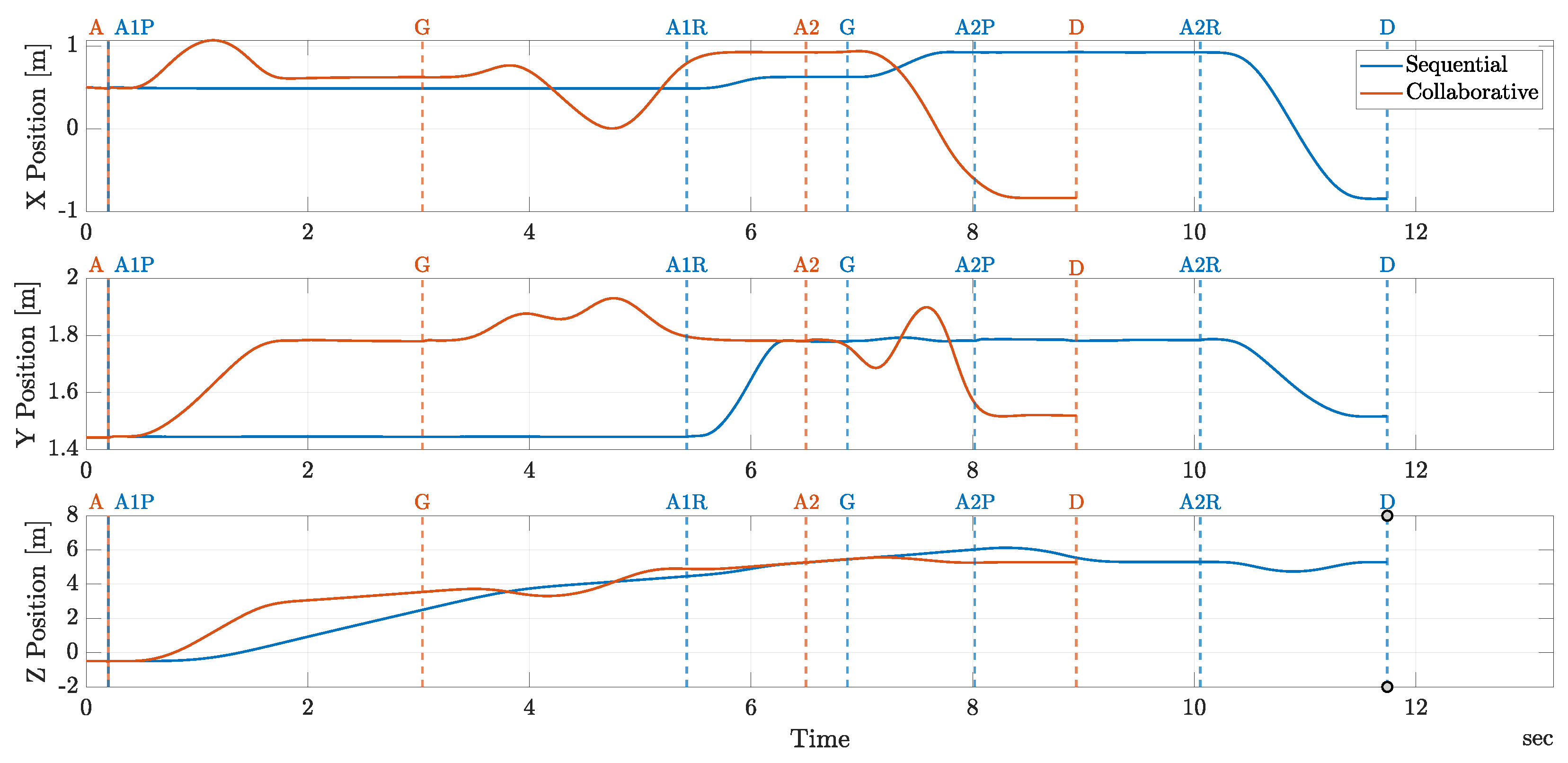
4. Use-Case Description

Robotic manipulators can be placed on an AGV or a 1-DOF or 2-DOF rail system or used as static standalone systems. Examples of common use cases are pick-and-place operations and work operations like welding, gluing, polishing, etc. In all cases, each joint follows a trajectory given by the OTP. The sub-task duration depends on the task type, mechanical limitations, and environment variables. In this study, a pick-and-place operation is used as a representative industrial task for comparing sequential and collaborative motion in modular manipulator systems. Specifically, the robot arm must pick up an object from the moving bottom sliding platform, then place it on an adjacent table. A Petri net representation of the collaborative version of this task is shown in Figure 5. The sequence has two ‘Align’ phases and two ‘Drop-off’ phases since the two modules execute their parts sequentially.

Multiple variations of the use case are considered. Five parameters are varied to obtain different sub-task durations. These parameters are the bottom platform speed (environment variable), a multiplier applied to the robot joints’ nominal velocity limits, another independent multiplier applied to the top platform nominal velocity limits, and the start delay. The bottom platform always starts at $t=0 \mathrm{s}$, effectively giving a head start.

Table 2. Range of use-case-defining parameters for simulation and experimental cases. $V_{lim}$ = nominal speed limit multiplier; BP = bottom platform; TP = top platform.

Environment	Case	BP [m/s]	TP Start [s]	Robot ${\mathit{V}}_{\mathit{lim}}$	TP ${\mathit{V}}_{\mathit{lim}}$
Sim.	1–5	$0.5$	1.2–5	$0.5$	1
	6–10	$0.5$	1.2–5	1	1
	11–15	$0.5$	1.2–5	1	$0.5$
	16–20	$0.5$	1.2–5	1	$1.2$
	21–25	$0.3$	1.2–5	$0.5$	1
	26–30	$0.3$	1.2–5	1	1
Exp.	1–5	$0.12$	1–5	1	1
	6–10	$0.12$	1–5	1	$0.5$
	11–15	$0.12$	1–5	$0.5$	1

shows the selected parameters for each case. An experiment with low robot velocity limits is representative of a real-world industrial task with work happening in a small radius. In this case, the robot arm is limiting execution time. Conversely, an experiment with a low top platform velocity limit is representative of a real-world industrial task where a robot has to travel a long distance between work operations. In this case, the top platform module is limiting execution time. The bottom platform (target object) speed and TP (top platform) start delay are additional variables used to vary the work–time ratio between both system modules.

Experimentally, three series of test cases with increasing start delays are run, again with variations in the top platform and robot arm speed limits. The bottom platform (and target object) cannot move as fast as in the simulation because the world model needs multiple consistent measurements to estimate speed reliably. This additional delay—combined with the OTP planning time and task execution time—causes the target object to reach the end of the track before the robot can effectively grab it. The selected speed of $0.12 \mathrm{m}/\mathrm{s}$ is the fastest target object speed that allows the experiments to reliably reach completion. The robot and top platform baseline speed limits are adjusted by a factor of 4 to keep the experimental and simulation baseline test cases comparable, i.e., in experimental cases 1–5, the robot and platform speed limits are divided by a factor of 4 compared to simulation cases 1–5.

5. Results and Discussion

5.1. Simulation Results

5.1.1. Singular Case Study

The task described in the paragraph above is executed in the simulation environment. The repeatability is evaluated by running the experiment multiple times. Variations are expected to occur due to the OTP having some degree of randomization. The experiment is executed five times for both collaborative motion and sequential motion. The means and standard deviations of sub-tasks and total execution times are recorded and displayed in

Table 3. Mean and standard deviation for simulation test case 3. Collaborative motion (top) and sequential motion (bottom), with 5 samples each. P = platform; R = robot.

Task	Mean [s]	$\mathit{\sigma }$ [s]	$\mathit{\sigma }$ [%]
Align 1	$4.987$	$0.022$	$0.43$
Grip	$1.044$	$0.002$	$0.16$
Align 2	$2.113$	$0.026$	$1.22$
Total	$8.143$	$0.029$	$0.35$
Task	Mean [s]	$\mathbf{\sigma }$ [s]	$\mathbf{\sigma }$ [%]
Align 1P	$5.778$	$0.022$	$0.38$
Align 1R	$1.236$	$0.004$	$0.29$
Grip	$1.025$	$0.002$	$0.21$
Align 2P	$1.887$	$0.029$	$1.53$
Align 2R	$1.465$	$0.003$	$0.21$
Total	$11.391$	$0.005$	$0.41$

. The task comprises three sub-tasks in collaborative mode. ‘Align 1’ is the concurrent movement of the robot and top platform to align the gripper with the target object. This sub-task is split into two tasks in sequential mode, namely, ‘Align 1P’ for the top platform and ‘Align 1R’ for the robot. ‘Grip’ is the action of grabbing the object. Then, ‘Align 2’ is the action of aligning the gripper with the target object to the drop-off location. In sequential mode, this action is also split. From these data, it is observed that the variation between simulation runs is very small, as the standard deviation stays below $1.5$% of the mean value, both for the sequential and collaborative sub-tasks and the total task. It can be concluded that the OTP’s randomization has a limited effect. It converges to a nearly identical solution every time, most probably due to the imposed kinematic constraints. For the remainder of the study on the simulation setup, a single run is performed. Given the slow simulation runtime (around $1 \mathrm{s}$ for one real-time minute), the planner compute time (around $1 \mathrm{s}$) is insignificant in the simulation and better studied in the experimental setup.

Figure 6 shows, for a single occurrence of simulation test case 3, the end-effector position for both collaborative (orange) and sequential (blue) motion. Parallel to the graphs, the specific timings for each sub-task are displayed. From Figure 6, it can be observed that the collaborative motion finishes faster than the sequential motion. Starting out, the planner generates a trajectory. Then, the end-effector aligns with the target object. For the collaborative scenario, this happens around $t=3 \mathrm{s}$, as shown by the dashed lines with the orange label ‘G’. In sequential motion, the platform first aligns around $t=5.5 \mathrm{s}$, as shown by the dashed line with blue label ‘A1R’, then the robot arm aligns around $t=6.5 \mathrm{s}$, as indicated by the dashed lines with blue label ‘G’. The time needed to perform the second action, i.e., dropping the object at a fixed location, depends on the execution of the first action. This interference can either increase or decrease the time difference between collaborative and sequential motion depending on the scenario. To keep a fair comparison between sequential and collaborative motion, only the time sequence of the first action is compared. The time saved by collaborative motion in this case is $6.5 \mathrm{s}$, or a $53.8$% saving.

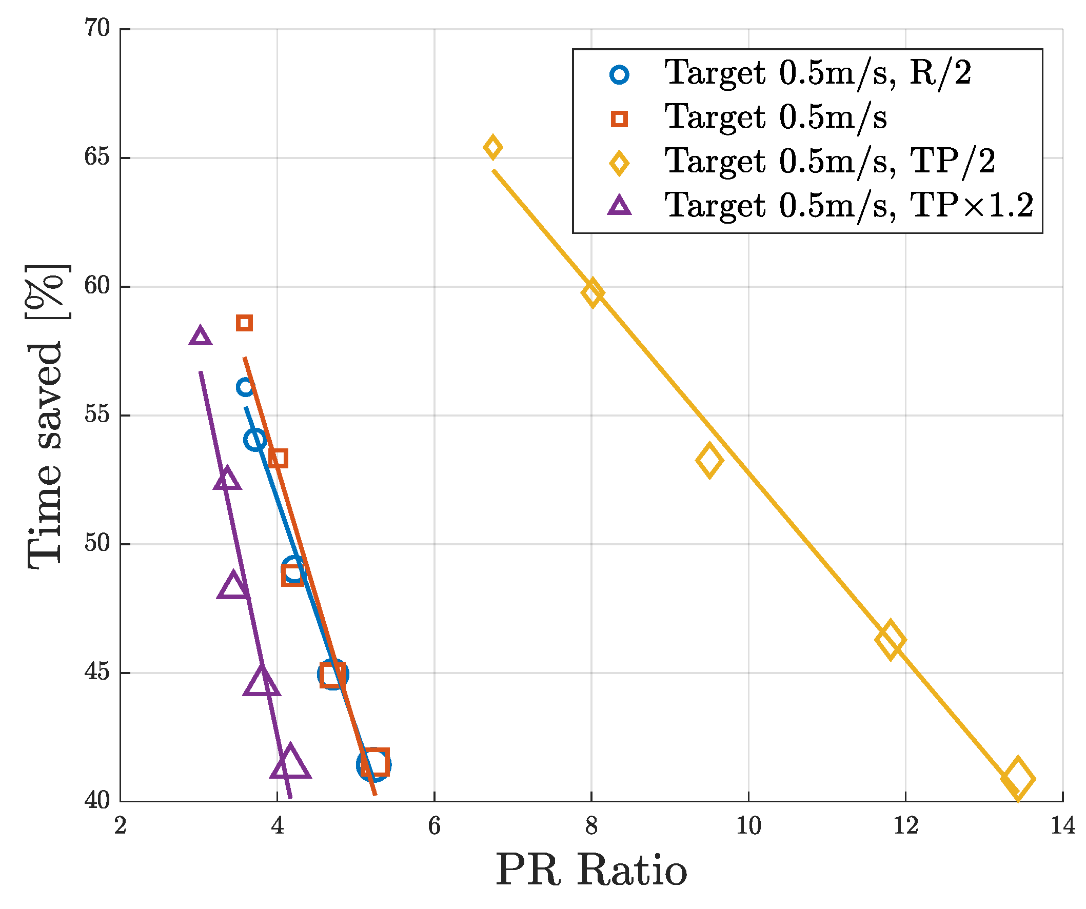
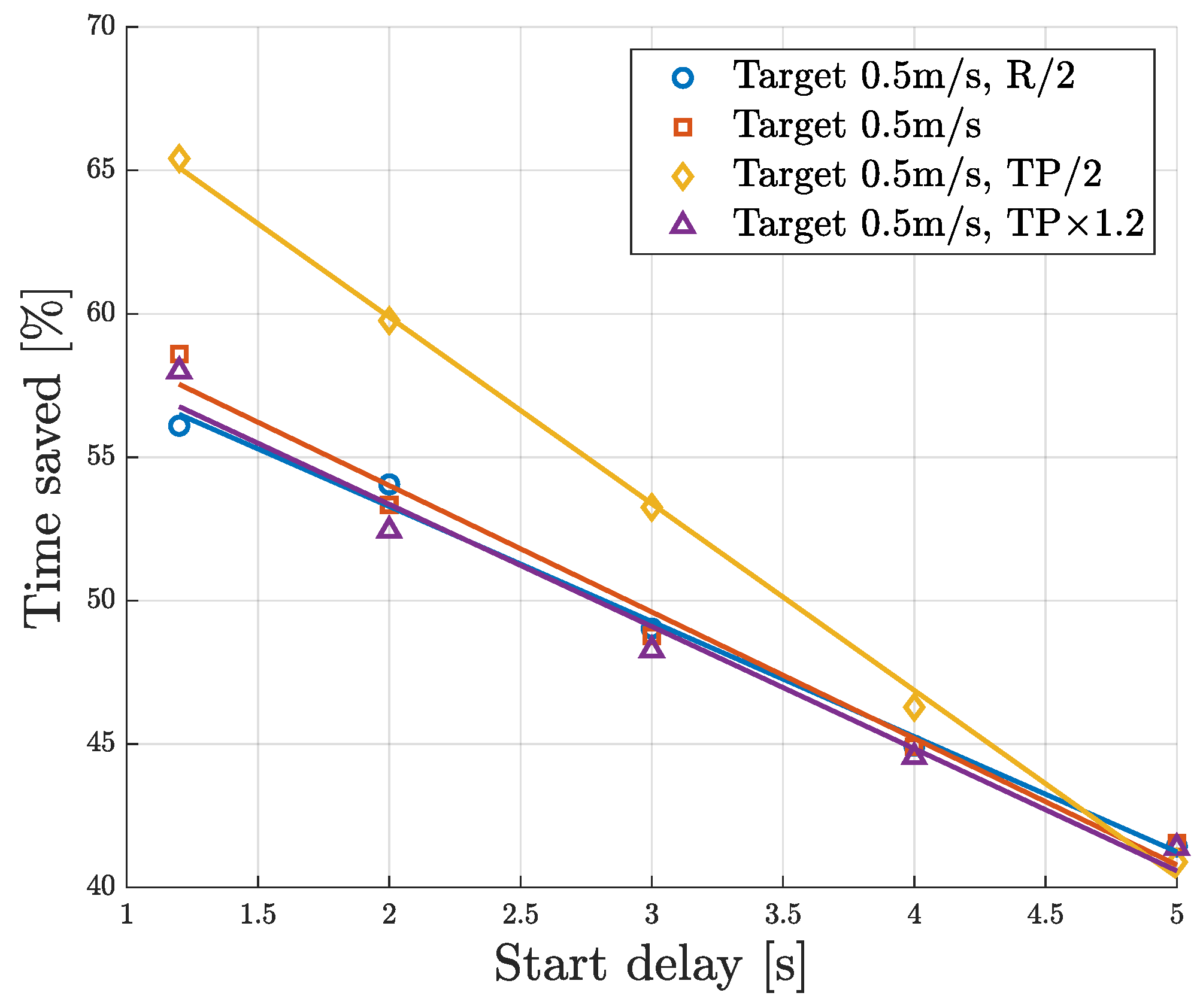
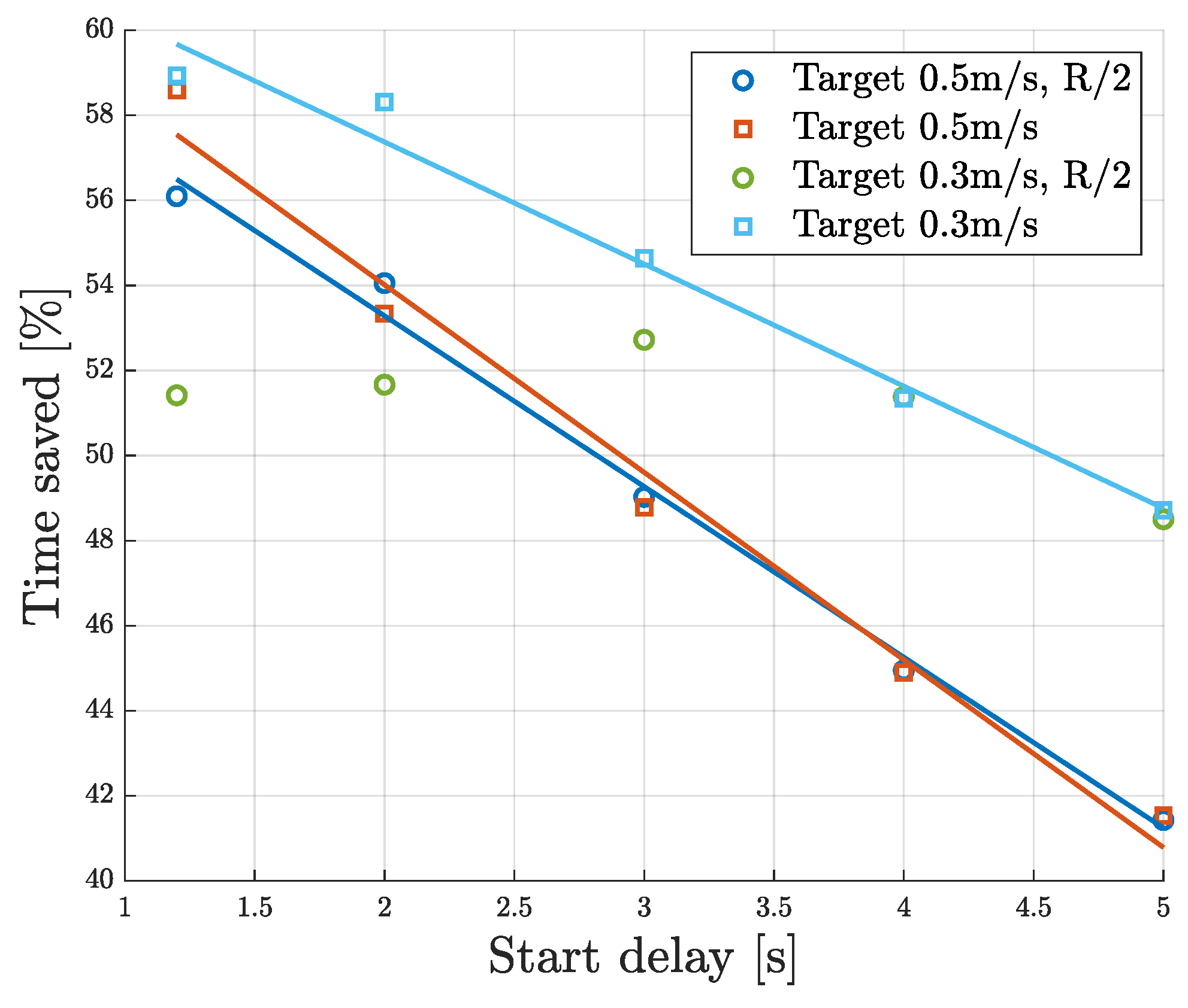
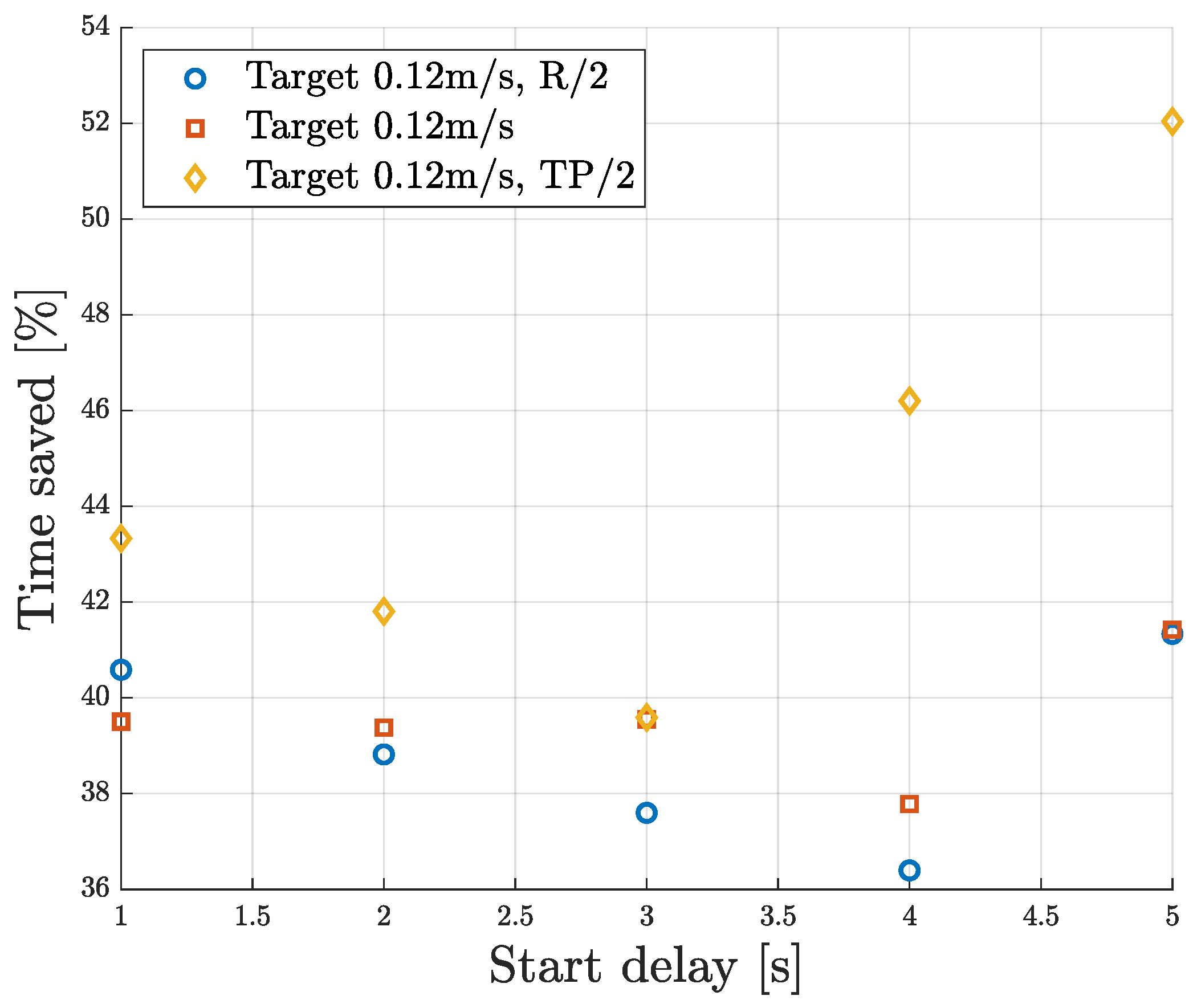
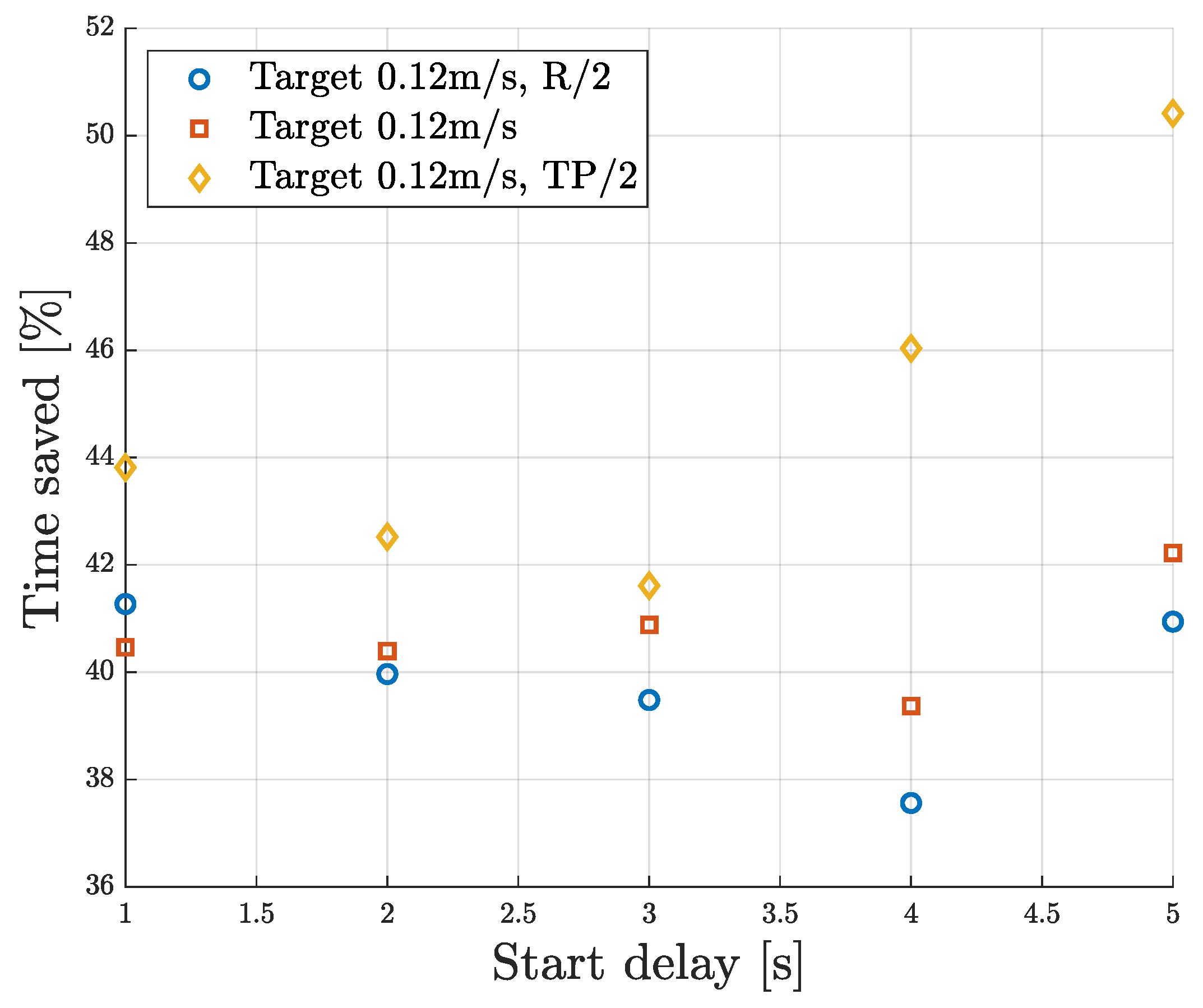
5.1.2. Sensitivity Analysis on Time Savings

This subsection analyzes the effects of varying the robot and top platform velocity limits on the time saved between sequential and collaborative motion. Let $PR$ be the ratio between the time it takes for the top platform to execute a sub-task and the time it takes to execute the analogous robot sub-task.

$$PR={\displaystyle \frac{T_{TP,seq}}{T_{R,seq}}}$$

Both sub-tasks occur sequentially. A PR ratio larger than one means the top platform is executing its sub-task for longer than the robot is. With the PR ratio, it is possible to compare tasks with similar relative time execution distributions but very different absolute durations. Intuitively, tasks with the same PR ratio should have the same time savings. Figure 7 shows the relation between PR ratio and the time saved (sequential versus collaborative motion) for cases 1 to 20 as defined in Table 2. Each color (and data point shape) represents a data series, as defined in the legend. The size of each data point is proportional to the top platform start delay ($1.2 \mathrm{s}$ to $5 \mathrm{s}$). From Figure 7, it is observed that the time saved for the 20 test cases is between 40% and 66%. However, the aforementioned hypothesis does not hold since the smallest orange square has the same PR ratio as the largest purple triangle but has around 15% greater relative time savings. This can be explained by absolute sub-task duration. The OTP has a fixed position tolerance for each DOF before validating a task end. The position and speed P and PI controllers approach the final OTP trajectory point asymptotically, meaning the ‘final approach’ time will be similar no matter how long the absolute sub-task duration. When the platform is very fast (purple triangles), the sub-tasks are very short with a relatively long ‘final approach’ time. In contrast, when the top platform is very slow (yellow diamonds), the ‘final approach’ is a much lesser proportion of the sub-task execution time. Nevertheless, in a given data series, time savings increase when the PR ratio decreases, as shown by the four linear regression lines shown in Figure 7.

Figure 8 shows the relation between the top platform start delay and time savings obtained for the four data series with the target object moving at $0.5 \mathrm{m}/\mathrm{s}$. It is observed that the time savings are inversely proportional to the start delay. For all four case series, when the start delay is $5 \mathrm{s}$ the time savings are approximately the same, around 42%. The slope is steepest when the top platform is limited to half its nominal speed and shallowest when the same condition is applied to the robot arm.

In the previous paragraph, the target was moving at a speed of $0.5 \mathrm{m}/\mathrm{s}$. Slowing down the target to $0.3 \mathrm{m}/\mathrm{s}$ while keeping the same range of top platform start delay gives a shorter start distance offset between the end-effector and target object. Figure 9 shows the first two case series for such a lower target object speed. The comparison between the two case series, with the nominal speed limits represented by squares, in Figure 9 shows a shallower regression line slope when the target object is slower. This implies a more constant time gain over the spread of tested start delays. The time gains are also larger in relative terms when the target object is slower. Depending on the test case conditions, when the start delay is very short, i.e., $1.2 \mathrm{s}$, the linear regression line fits poorly. This is already visible in both the dark- and light-blue data series, as the point at $1.2 \mathrm{s}$ is significantly below the linear regression line. This is even more evident when the robot speed limits are halved and the target object moves slowly (green circles). This data series and the linear trend of the other series suggest a saturation of time saving when the task becomes very short. The slow asymptotic final approach behavior of the position and speed controllers described previously could also explain this saturation effect.

To reduce this slow asymptotic final approach to the setpoint, two solutions arise. First, the end-of-task tolerance can be increased, offering coarser positioning. It then becomes a balancing act specific to the application between precision and speed of task execution. Secondly, the controller gains can be adapted in real time based on the error size to obtain more aggressive control when the error is small. This brings system stability risks and takes an additional tuning effort.

5.2. Experimental Results

5.2.1. Analysis of Task Execution Time

Figure 10 shows the time saved by collaborative motion compared to sequential motion on the experimental setup in relation to the top platform start delay. The time savings are average values taken from five attempts at each test case. For a more direct comparison with the simulation data (in which computing time is very small in relative terms), this figure isolates the execution time and excludes any computation time needed to generate the trajectories. The next paragraph analyses the experimental data inclusive of the computing time. First, it can be observed that the time savings are generally lower as they range from 52% to 36%, while they ranged from 65% to 40% in the simulation. Similarly to the simulation test cases, the time savings are greatest when the top platform is slow and lowest when the robot arm is slow. The trend of decreasing time savings with increasing start delay, consistently observed in the simulation, is only seen experimentally for start delays between $1 \mathrm{s}$ and $3 \mathrm{s}$. For longer start delays, the experimental graph suggests an increasing time saving trend when the start delay increases. Due to the large standard deviations associated with the obtained average values, around 10%, the aforementioned trends are uncertain.

While the planner’s computation time is insignificant in the simulation, it is a significant proportion of the experimental test cases’ durations. Since the planner computes a new trajectory at the end of the preceding task and since there are double the planning occurrences in sequential mode compared to collaborative mode, it is expected for the planning time to be halved for the collaborative cases. However, since trajectories for more DOFs are computed in collaborative mode (seven instead of six or one), it is expected that this planning occurrence will take longer than a single occurrence of the planning in sequential mode. The planning time saved by collaborative motion ranges from $39.2$% to $48.8$% and is on average $44.7$%. Figure 11 shows the measured time saved, including both execution and planning time, by collaborative motion compared to sequential motion for a range of test cases. The time savings are generally within a percent of the pure execution time savings shown in the previous figure. For this set of data, the computing time has little impact on the relative time savings. However, in absolute terms the time saved is still significant, i.e., around $1.44 \mathrm{s}$ in collaborative mode versus $2.60 \mathrm{s}$ in sequential mode.

5.2.2. Energy Sustainability Study

While the time efficiency of an industrial process is analyzed in the previous subsection, energy use also plays a role in the cost-effectiveness of collaborative motion. The same test cases are analyzed for purely mechanical energy demand.

With the energy used by the total system computed by

$$E\left(t_i\right)=\sum _{i=1}^N{P}_T\left(t_i\right)\Delta t$$

where

• $\Delta t=250 \mathrm{\mu }\mathrm{s}$ is the simulation timestep;
• $P_T\left(t_i\right)=P_{TP}\left(t_i\right)+{\sum }_{j=1}^6{P}_{Jj}\left(t_i\right)$;
• N is the number of timesteps for a sub-task.

The instantaneous mechanical power needed at each joint is the product of instantaneous torque and rotational velocity, as seen by the (emulated) motor:

$$P\left(t_i\right)=T\left(t_i\right)·\omega \left(t_i\right)$$

Figure 12 shows the energy consumption of the robot and top platform during each test case for the collaborative case on the y-axis and the sequential case on the x-axis. For each test case (five attempts), the mean value is displayed with the corresponding standard deviations. The line $y=x$ is represented in black on the graph and represents equal energy consumption in collaborative and sequential modes. All data points fall below the reference line, indicating energy savings, of $35.2$% on average, in collaborative mode compared to sequential cases. The major part of the mechanical energy consumption comes from the top platform motion, since it is moving throughout the whole experiment: first to align, then to track the moving target object. Comparatively, the robot arm solely moves during its own alignment task. Additionally, during the test cases, the robot moves from a higher-potential-energy state to a lower-potential-energy state due to gravity. Therefore, some joints are assisted by gravity (negative energy) while others move against it (positive energy), giving a relatively low balance of energy compared to the energy use of the top platform. A linear regression applied to the robot’s energy consumption, analogous to the cloud of points shown in Figure 12, shows an equivalent robot arm energy consumption between corresponding sequential and collaborative test cases. The robot motion is in fact very similar in collaborative and sequential motion. Therefore, the total energy consumption difference is explained mainly by the longer duration and thus longer moving time of the top platform in sequential mode. It can be concluded that the energy savings are principally due to the time savings shown in the previous section.

6. Conclusions

This study has quantified the performance benefits of collaborative motion compared to sequential motion in modular mechatronic systems for pick-and-place operations, addressing a gap in the existing literature. Through both simulation and experimental validation, it was demonstrated that coordinated operation of modular robotic systems can yield significant improvements in operational efficiency and energy consumption. Specifically, the results indicate time savings ranging from 36% to 52%, with an approximate reduction in energy consumption of 35%. These findings are limited to a single experimental setup for pick-and-place operations, representative of a vast amount, but not all, of industry-relevant test cases. It is the authors’ belief that these results would extrapolate to other types of industrial operations with similar motion patterns. For tasks with different motion patterns (lots of static time, for example), the time gain is expected to be greatly reduced. The study findings highlight the importance of control and perception systems tailored to modular mechatronic systems. With these, modular mechatronic systems can perform to the level of non-modular equivalent systems while benefiting from the modular system advantages (increased flexibility, cost-effectiveness, reconfigurability). Future research could study types of industrial operations other than pick-and-place actions. Furthermore, a system with more DOFs or a very different kind of motion could be studied; for example, a drone or AGV-mounted robotic arm. The tests could be repeated in the presence of dynamic obstacles and a continuously variable target object speed, requiring re-planning during task execution. The benefits of adaptive control of modular systems could also be studied. The effect of distributed control algorithms on the time and energy savings could also be investigated.

References

1. Rikalovic, A.; Suzic, N.; Bajic, B.; Piuri, V. Industry 4.0 Implementation Challenges and Opportunities: A Technological Perspective. IEEE Syst. J. 2022, 16, 2797–2810. [Google Scholar] [CrossRef]
2. Zou, Y.; Kim, D.; Norman, P.; Espinosa, J.; Wang, J.C.; Virk, G.S. Towards robot modularity—A review of international modularity standardization for service robots. Robot. Auton. Syst. 2022, 148, 103943. [Google Scholar] [CrossRef]
3. Kumar, S.; Raut, R.D.; Narwane, V.S.; Narkhede, B.E. Applications of industry 4.0 to overcome the COVID-19 operational challenges. Diabetes Metab. Syndr. Clin. Res. Rev. 2020, 14, 1283–1289. [Google Scholar] [CrossRef]
4. Sundarkumar, V.; Wang, W.; Mills, M.; Oh, S.W.; Nagy, Z.; Reklaitis, G. Developing a Modular Continuous Drug Product Manufacturing System with Real Time Quality Assurance for Producing Pharmaceutical Mini-Tablets. J. Pharm. Sci. 2024, 113, 937–947. [Google Scholar] [CrossRef] [PubMed]
5. Riesener, M.; Kuhn, M.; Boßmann, C.; Schuh, G. Methodology for the Design of Interdisciplinary Modules for Mechatronic Modular Product Platforms. Procedia CIRP 2023, 119, 675–680. [Google Scholar] [CrossRef]
6. Janssen, L.A.L.; Fey, R.H.B.; Besselink, B.; Wouw, N.v. Modular redesign of mechatronic systems: Formulation of module specifications guaranteeing system dynamics specifications. Mechatronics 2024, 103, 103236. [Google Scholar] [CrossRef]
7. Seidenberg, T.; Disselkamp, J.-P.; Jürgenhake, C.; Grobbel, D.; Dumitrescu, R.; Papanikolaou, A. Development of a modular architecture for complex mechatronic systems. In Proceedings of the 33rd CIRP Design Conference, Sydney, Australia, 17–19 March 2023. [Google Scholar]
8. Grosz, E.A.; Borzan, M. Modular Robotics Configurator: A MATLAB Model-Based Development Approach. Appl. Syst. Innov. 2024, 8, 21. [Google Scholar] [CrossRef]
9. Choi, L.; Choi, M.; Kwon, S.; Youn, D.; Song, G. Modular production of small ship models using 3D printing for model tests. Ocean. Eng. 2024, 302, 117685. [Google Scholar] [CrossRef]
10. Kern, W.; Rusitschka, F.; Bauernhansl, T. Planning of Workstations in a Modular Automotive Assembly System. Procedia CIRP 2016, 57, 327–332. [Google Scholar] [CrossRef]
11. Hossain, M.S.; Chakrabortty, R.K.; Elsawah, S.; Ryan, M.J. Hierarchical joint optimization of modular product family and supply chain architectures considering sustainability. Sustain. Prod. Consum. 2023, 43, 15–33. [Google Scholar] [CrossRef]
12. Wang, X.; Liu, W.; Wu, Q.; Li, S. A Modular Optimal Formation Control Scheme of Multiagent Systems With Application to Multiple Mobile Robots. IEEE Trans. Ind. Electron. 2023, 69, 9331–9341. [Google Scholar] [CrossRef]
13. Mo, F.; Rehman, H.U.; Monetti, F.M.; Chaplin, J.C.; Sanderson, D.; Popov, A.; Maffei, A.; Ratchev, S. A framework for manufacturing system reconfiguration and optimisation utilising digital twins and modular artificial intelligence. Robot. Comput. Integr. Manuf. 2023, 82, 102524. [Google Scholar] [CrossRef]
14. Gros, J.; Zatyagov, D.; Papa, M.; Colloseus, C.; Ludwig, S.; Aschenbrenner, D. Unlocking the Benefits of Mobile Manipulators for Small and Medium-Sized Enterprises: A Comprehensive Study. Procedia CIRP 2023, 120, 1339–1344. [Google Scholar] [CrossRef]
15. Amertet, S.; Gebresenbet, G.; Alwan, H.M. Optimizing the performance of a wheeled mobile robots for use in agriculture using a linear-quadratic regulator. Robot. Auton. Syst. 2024, 174, 104642. [Google Scholar] [CrossRef]
16. Sayar, E.; Gao, X.; Hu, Y.; Chen, G.; Knoll, A. Toward coordinated planning and hierarchical optimization control for highly redundant mobile manipulator. ISA Trans. 2024, 146, 16–28. [Google Scholar] [CrossRef] [PubMed]
17. Ye, L.; Wu, F.; Zou, X.; Li, J. Path planning for mobile robots in unstructured orchard environments: An improved kinematically constrained bi-directional RRT approach. Comput. Electron. Agric. 2023, 215, 108453. [Google Scholar] [CrossRef]
18. Ristevski, S.; Cakmakci, M. Planar motion controller design for a modular mechatronic device with heading compensation. Mechatronics 2019, 62, 102257. [Google Scholar] [CrossRef]
19. Jiang, Z.; Chen, Z.; Xu, K.; Shi, L. Distributed collaborative control to pose tracking for six-DOF parallel mechanism under multi-cylinder communication. ISA Trans. 2025, 159, 312–325. [Google Scholar] [CrossRef]
20. Sekban, H.T.; Basci, A. Designing New Model-Based Adaptive Sliding Mode Controllers for Trajectory Tracking Control of an Unmanned Ground Vehicle. IEEE Access 2023, 11, 101387–101397. [Google Scholar] [CrossRef]
21. Liu, W.; Liu, C.; Liang, X.; Zheng, M. A hybrid task-constrained motion planning for collaborative robots in intelligent remanufacturing. Mechatronics 2024, 102, 103222. [Google Scholar] [CrossRef]
22. Saeed, M.; Demasure, T.; El-Houssaine, A.; Cottyn, J. Optimization-based estimation of the execution time of a robotic assembly task sequence. Int. J. Adv. Manuf. Technol. 2024, 130, 5315–5328. [Google Scholar] [CrossRef]
23. Peta, K.; Wiśniewski, M.; Kotarski, M.; Ciszak, O. Comparison of Single-Arm and Dual-Arm Collaborative Robots in Precision Assembly. Appl. Sci. 2025, 15, 2976. [Google Scholar] [CrossRef]
24. Angleraud, A.; Mehman Sefat, A.; Netzev, M.; Pieters, R. Coordinating Shared Tasks in Human-Robot Collaboration by Commands. Front. Robot. AI 2021, 8, 734548. [Google Scholar] [CrossRef] [PubMed]
25. Calvo, R.; Gil, P. Evaluation of Collaborative Robot Sustainable Integration in Manufacturing Assembly by Using Process Time Savings. Materials 2022, 15, 611. [Google Scholar] [CrossRef]
26. Papanastasiou, S.; Kousi, N.; Karagiannis, P.; Gkournelos, C.; Papavasileiou, A.; Dimoulas, K.; Baris, K.; Koukas, S.; Michalos, G.; Makris, S. Towards seamless human robot collaboration: Integrating multimodal interaction. Int. J. Adv. Manuf. Technol. 2019, 105, 3881–3897. [Google Scholar] [CrossRef]
27. Polonara, M.; Romagnoli, A.; Biancini, G.; Carbonari, L. Introduction of Collaborative Robotics in the Production of Automotive Parts: A Case Study. Machines 2024, 12, 196. [Google Scholar] [CrossRef]
28. Polonara, M.; Carbonari, L.; Romagnoli, A.; Biancini, G. Collaborative Mobile Robotics for SMEs: A Case Study. In Proceedings of the 2024 20th IEEE/ASME International Conference on Mechatronic and Embedded Systems and Applications (MESA), Genova, Italy, 2–4 September 2024. [Google Scholar]
29. Faccio, M.; Bottin, M.; Rosati, G. Collaborative and traditional robotic assembly: A comparison model. Int. J. Adv. Manuf. Technol. 2019, 102, 1355–1372. [Google Scholar] [CrossRef]
30. Carlier, R.; Gillis, J.; Rademakers, E.; Borghesan, G.; Clercq, P.D.; Ganseman, C.; Stockman, K.; Kooning, J.D.M.D. A Digital Twin Framework for Virtual Re-Commissioning of Work-Drive Systems Using CAD-based Motion Co-Simulation. In Proceedings of the 2023 IEEE/ASME International Conference on Advanced Intelligent Mechatronics (AIM), Seattle, WA, USA, 28–30 June 2023. [Google Scholar]
31. Gillis, J.; Vandewal, B.; Pipeleers, G.; Swevers, J. Effortless modeling of optimal control problems with rockit. In Proceedings of the 39th Benelux Meeting on Systems and Control, Elspeet, The Netherlands, 10–12 March 2020. [Google Scholar]
32. Andersson, J.A.E.; Gillis, J.; Horn, G.; Rawlings, J.B.; Diehl, M. CasADi–A software framework for nonlinear optimization and optimal control. Math. Program. Comput. 2019, 11, 1–36. [Google Scholar] [CrossRef]
33. Gillis, J.; Pipeleers, G.; Swevers, J. Effortless modeling of optimal control problems with rockit. In Proceedings of the 41st Benelux Meeting on Systems and Control, Brussels, Belgium, 5–7 December 2020. [Google Scholar]
34. Wächter, A.; Biegler, L.T. On the implementation of an interior-point filter line-search algorithm for large-scale nonlinear programming. Math. Program. 2006, 106, 25–57. [Google Scholar] [CrossRef]
Figure 1. Schematic of control and vision software architecture for the simulation model.
Machines 13 00348 g001
Figure 2. CAD representation of the robot arm and sliding platforms.
Machines 13 00348 g002
Figure 3. Picture of robotic arm with gripper attached to the top platform.
Machines 13 00348 g003
Figure 4. Picture of the Aruco markers on the target object and the bottom sliding platform.
Machines 13 00348 g004
Figure 5. Petri net showing the task sequence for the collaborative motion.
Machines 13 00348 g005
Figure 6. Graph showing the robot end-effector position with the task decomposition for collaborative and sequential motion in the simulation test case 3.
Machines 13 00348 g006
Figure 7. Time saved by collaborative motion versus sequential motion correlated with PR ratio.
Machines 13 00348 g007
Figure 8. Time saved by collaborative motion versus sequential motion correlated with start delay. Highlighting the effect of top platform and robot speed limits.
Machines 13 00348 g008
Figure 9. Time saved by collaborative motion versus sequential motion correlated with start delay. With fast and slow target object speed cases.
Machines 13 00348 g009
Figure 10. Time saved by collaborative motion versus sequential motion for the experimental test cases, excluding path computation time.
Machines 13 00348 g010
Figure 11. Time saved by collaborative motion versus sequential motion for the experimental test cases, including path computation time.
Machines 13 00348 g011
Figure 12. Energy consumption of robot and top platform for each experimental test case.
Machines 13 00348 g012