Abstract
This paper explores the feasibility and implications of developing a privacy-preserving, data-driven cloud service for predicting the energy consumption of industrial robots. Using machine learning, we evaluated three neural network architectures—dense, LSTM, and convolutional–LSTM hybrids—to model energy usage based on robot trajectory data. Our results show that models incorporating manually engineered features (angles, velocities, and accelerations) significantly improve prediction accuracy. To ensure secure collaboration in industrial environments where data confidentiality is critical, we integrate privacy-preserving machine learning (ppML) techniques based on secure multi-party computation (SMPC). This allows energy inference to be performed without exposing proprietary model weights or confidential input trajectories. We analyze the performance impact of SMPC on different network types and evaluate two optimization strategies, using public model weights through permutation and evaluating activation functions in plaintext, to reduce inference overhead. The results highlight that network architecture plays a larger role in encrypted inference efficiency than feature dimensionality, with dense networks being the most SMPC-efficient. In addition to model development, we identify and discuss specific stages in the MLOps workflow—particularly model serving and monitoring—that require adaptation to support ppML. These insights are useful for integrating ppML into modern machine learning pipelines.
1. Introduction
The growing emphasis on energy efficiency in production processes is driven by increasing operational costs and stringent environmental regulations. Industrial production systems consume a significant amount of energy, making energy modeling a critical tool for optimizing resource utilization [1]. Among production systems, industrial robots are a key feature due to their widespread adoption and energy demands in automated workflows [2]. Modeling such systems, especially with the use of deep learning, might require extensive amounts of data and computational resources. These resources can often be accessed through modern cloud infrastructure and frequently involve sharing sensitive operational data during collaboration. In collaborative industrial environments, privacy-preserving machine learning (ppML) is emerging as a key methodology to ensure secure collaboration on data gathering while protecting intellectual property across diverse applications.In this work we aim to develop a comprehensive understanding and framework for integrating data-driven energy modeling with ppML in a seamless way along the development life cycle in order to enable easy development of novel collaborative cloud-based use cases for smart manufacturing. This paper is an extended version of our paper published in [3].
1.1. Motivation
Energy models offer significant value, but their deployment can involve sharing sensitive intellectual property (e.g., neural network weights or trajectory data). This poses challenges in collaborative environments where multiple stakeholders—such as manufacturers and third-party service providers—must interact without exposing proprietary information. Generally speaking, there has been a significant surge in machine learning adoption in the industrial sector, with applications ranging from predictive maintenance to process optimization. As these ML models grow increasingly sophisticated, their computational demands have led to a paradigm shift toward cloud-based solutions typically managed by third-party service providers. This transition, while offering substantial computational benefits, introduces notable privacy and security concerns for industrial stakeholders. Privacy-preserving machine learning (ppML) is a promising solution to address these challenges. ppML encompasses techniques and methodologies designed to protect both the confidentiality of training data and the privacy of model parameters during the training and inference phases. The primary objective is to prevent unauthorized access to sensitive information while maintaining the functionality and performance of ML models.
The motivations for this work are twofold. One the one hand, based on preliminary findings [3], we want to demonstrate the capabilities of ppML in robotics. Through extensive benchmarking of different models to solve a particular use case, we explore the practicability of SMPC for industrial applications in general. The results should help developers of industrial cloud-based services and platforms to estimate the overhead of end-to-end security and provide ways to optimize performance. On the other hand, we want to deliver a blueprint for the development of privacy-preserving applications themselves, such as the one visualized in Figure 1, thus streamlining the software development and ppML integration processes for application developers. Only if the development process is integrated into the design methodology will it be feasible for non-experts in secure computation techniques to leverage the potential of ppML and thus design novel collaborative use cases based on data for future production systems.
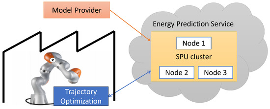
Figure 1.
High-level overview of a cloud-based energy prediction use case integrating a privacy-preserving SMPC workflow [3].
1.2. Related Work
In the following section we discuss the state of the art in the two main fields relevant for our work, i.e., the work that has been conducted on data-driven energy modeling in manufacturing and the field of privacy-preserving computing for machine learning.
1.2.1. Energy Modeling
For modeling the energy consumption of industrial processes, several approaches have been utilized including (i) analytical modeling where energy demand is modeled by analyzing different operation modes (e.g. on, off, idle, etc.) and defining the energy consumption of each mode, usually represented as an average demand; (ii) empirical modeling, which commonly uses multiple linear regression to fit a predefined mathematical expression that is linear in the models’ parameters; (iii) physical modeling where fundamental physical relationships are expressed in mathematical equations; (iv) machine learning methods, which utilize data-driven algorithms to identify relationships between input and output data [4]. For analytical modeling, oversimplification can be considered as a possible drawback, while for empirical modeling it can be difficult to find the right mathematical expression that fits the collected data [4]. Physics-based models can be very accurate, but they are often difficult to implement and require a high level of insight and expertise about the problem to be modeled [1,4]. Data-driven approaches such as neural networks offer a flexible alternative that harnesses network approximation capabilities, although with acknowledged tradeoffs in terms of accuracy and extrapolation compared to, e.g., physics-based models.
Concerning energy consumption modeling for industrial robots, research was conducted based on the development of a physical model [5,6,7], which commonly requires the identification of parameters for robot dynamics and parameters describing power losses due to, e.g., friction, copper losses in the motors or losses in the control system. For dynamic parameter identification torque measurements must usually be obtained [8,9,10]. However, for some industrial robots, it is not trivial to determine the torque of the robot axis, which is addressed in [5], where the dynamic robot parameters are identified based only on the total electrical power consumption. In [11], modeling is performed using the Modelica language, while dynamic parameters are obtained from documentation and related studies. Works applying data-driven approaches to the robotic energy modeling problem include strategies such as the utilization of neural networks for determining operation parameters and optimizing energy consumption. Zhang and Yang [12] use a feedforward neural network to determine the operating parameters of maximum velocity and acceleration with a focus on minimizing total energy consumption on a given path and type of motion. Yin [13] et al. used a deep neural network for modeling and optimizing the energy consumption of a robot on a simplified case study. In [1], different states of operation are identified which are the approximated using linear regression.
In general, energy modeling using machine learning techniques has provided promising results and is increasingly applied in industrial manufacturing processes. However, regarding energy modeling for IRs, more research needs to be conducted in terms of case studies on real applications and by applying different machine learning algorithms in order to compare their performance.
1.2.2. Privacy-Preserving Machine Learning
The concept of SMPC was invented more than 30 years ago, but for a long time, it was considered only of theoretical interest. However, progress in recent years has led to many interesting applications which can be realized with practical efficiency (e.g., as in [14,15]). Some SMPC frameworks with general use-cases like MPyC (https://github.com/lschoe/mpyc (accessed on 7 January 2025)) support simple neural networks or MP-SPDZ [16], which enables simple neural networks or the importing of neural networks from well-known frameworks like PyTorch 2.8. This progress, along with the popularity of deep-neural network usage, has led to the development of many SMPC frameworks developed specifically for neural network usage.
SecretFlow-SPU [17] is a multi-party computation (MPC) framework suitable for machine learning that currently supports three MPC protocols, namely ABY3 [18], Semi2k-SPDZ [19], and Cheetah [20]. ABY3 [18] is a framework for ppML across three servers using secure three-party computation. The framework enables efficient conversion between arithmetic, binary, and Yao computation methods, incorporating new techniques for fixed-point multiplication and polynomial time evaluation. CrypTen [21] is an MPC-enabling framework for machine learning. It utilizes a semi-honest threat model and abstracts many MPC primitives in the form of tensor computation, automatic differentiation, and many widely used neural network layers.
1.3. Contribution and Structure
This paper significantly extends preliminary work from [3]. Specifically, the contributions are, first, a comprehensive research and evaluation of data-driven energy prediction for industrial robots with high accuracy based on small models for later ppML integration; second, a comprehensive analysis of ppML integration for the given models specifically considering performance optimization and privacy–security trade-offs; and third, an analysis and discussion of ppML integration into MLOps workflow to support seamless development for non-security experts in support of future applications.
To achieve this, we first develop a neural network-based prediction model for energy consumption. We then apply ppML methods to these models to achieve data safety and integrity in collaborative environments. Finally, we investigate and locate the parts of the MLOps pipeline that would require attention specific to ppML integration.
The remainder of the paper is structured as follows: In Section 2 the process of acquiring the data for training and testing from the industrial robot is explained, followed by Section 3 where feature engineering, data preprocessing, and different model architectures developed are shown. In Section 4 the framework for privacy-preserving energy prediction is introduced along with a brief explanation of the two optimization methods used for decreasing inference times in the ppML domain. Next, in Section 5 an analysis of the developed model’s results is conducted in both plaintext and ppML forms, followed by Section 6, where MLOps is introduced, and its required changes for ppML integration are discussed. Section 7 concludes this paper.
2. Data Acquisition
In this section a developed method for robot data acquisition is presented in detail, as dedicated hardware and software were necessary to acquire data with high accuracy and quality.
2.1. Boundary Conditions
The system for which energy consumption is to be modeled is the seven-axis collaborative industrial robot LBR iiwa R800, developed by KUKA Germany GmbH, Augsburg, Germany. The main components of the robotic system are depicted in Figure 2a. The robot is integrated into a laboratory setup that simulates a production line, where it is employed for assembly and handling tasks. Robot applications and motion programming are developed using the KUKA Sunrise.Workbenchdevelopment environment. Within this environment, the KUKA RoboticsAPI is available, offering functionalities for motion planning, execution, and data recording.
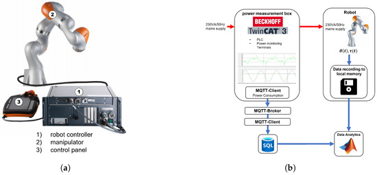
Figure 2.
Data acquisition model components and structure [3]. (a) Components of the robotic system (adapted from [22]); (b) general structure of the measurement concept.
2.2. Data Acquisition
To enable the development of data-driven models, it is essential to first collect meaningful data that captures relevant aspects of the system’s behavior. For the problem addressed in this work, the relevant data includes
- Robot axis angles over time,
- Consumed electrical active power,
The measurement concept designed to obtain data from both the electrical and mechanical domains is illustrated in Figure 2b. The figure outlines the general structure and operational principle of the data acquisition setup. The flow of electrical energy is represented by red arrows moving from left to right. As shown, the robot’s electrical supply passes through an additional power measurement box, which measures the robot’s power consumption. For power measurement, voltage and current are sampled at a rate of 20,000 and aggregated over two mains supply periods, corresponding to ms. These aggregated values are then used to compute the active power. Mechanical data is captured using functions provided by the KUKA RoboticsAPI, which logs motion data directly to a file. From the mechanical domain, axis angles and measured axis torques are recorded at a sampling interval of 40 ms. The mechanical data flow is indicated by blue arrows. Electrical data is transmitted using the MQTT network protocol and stored in a central SQL database. Both the data collected from the database and from the robot controller are subsequently available for further analysis.
2.3. Trajectory Generation and Execution
Sufficient excitation is necessary to obtain enough data for the creation of accurate models by machine learning. To this end, we use two different methods to generate trajectories suitable for excitation, namely
- Limited Space Random (LimSp)—where random positions within a defined subspace of all reachable manipulator poses are generated. The orientation of the end-effector was fixed.
- All Space Random (AllSp)—where random robot configurations, i.e., axis angles, are generated using the entire configuration space of the robot. Valid robot configurations are subject to physical constraints, e.g., collisions with environment.
Limited Space Random has the advantage that trajectories can be generated more easily and that models, due to reduced complexity, can faster mimic system behavior. However, such models are likely to not perform well outside the provided training data by extrapolation. To develop models that generalize well over all possible robot movements and to test the limitations of the models obtained by Limited Space data, the All Space data is generated as well.
For both methods, we created several trajectories (46 Lim.Sp., 30 AllSp.) and stored their robot configuration, which can be later used as inputs for execution on the real robot. Trajectories were executed as ptp motions between given positions. To get additional variability and to produce more data out of the same source trajectories, each motion is executed with a random blending factor and random velocity. Figure 3 shows an example of one LimSp. and one AllSp. trajectory, with the effect of blending also shown. For Limited Space data 202 recordings corresponding to 2.8 h recording time were made; for All Space 135 recordings and 2.7 h.
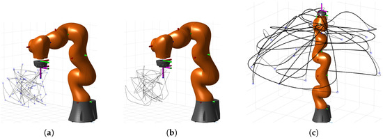
Figure 3.
Effect of relative blending factor: (a)—example of Limited Space Random points indicated with circles and the ptp motion between points as a solid line; (b)—recordings when trajectory (a) is executed with blending; (c)—example of All Space Random points indicated as circles, ptp motion as a solid line, and recorded motion as a dotted fat line. Taken from [3].
2.4. Data Preparation and Analysis
The data was recorded by two different systems: the electrical data from the measurement box and the mechanical data from the robot controller. Each of these systems operates independently, resulting in both systems generating their own timestamps, so the measurements must be combined using an appropriate method. To this end, the obtained time series are combined with a common time vector with sampling interval using linear interpolation between points.
In addition to merging of the data, we also examined how the time series fit together by observing distinctive patterns in the data. For comparison of the electrical and mechanical data, the mechanical power is calculated with the angular velocity and measured axis torque (1).
Angular velocity is calculated out of the measured axis angles by calculating the first-order centered finite difference (2).
Figure 4 top shows the resulting mechanical and electrical power of a selected measurement. Apart from the initial peak, attributed to inrush currents, the results are similar in amplitude and course, but a considerable shift in time can be observed.
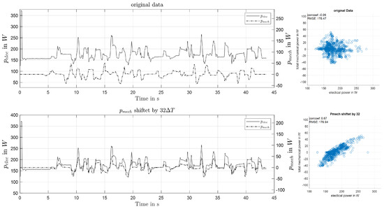
Figure 4.
Comparison of shifted and non-shifted power sequences.
This time difference in the acquired data can be attributed to non-synchronized clocks of the measurement systems. To compensate for this overall offset, or lag, the cross-correlation of the two time series was calculated, and the time difference to compensate for was determined as the lag at which cross-correlation becomes maximal. Figure 4 shows an example of the original and the shifted data. The sequences are shown in the time domain along with a scatter plot for visualizing the correlation.
3. Model Development
In the following section the development of energy models is assessed for our case studies. The used modeling approaches are based on machine learning techniques as well as neural networks. Multiple network architectures are explored, including long short-term memory (LSTM) networks with engineered features as inputs, LSTM networks using a convolutional head for automated feature extraction, and dense networks. Specifically, we train neural networks based on certain input features derived from robot trajectory data to predict the energy consumption in a sequence-to-sequence-based problem.
3.1. Feature Engineering
To select suitable features, we will first take a closer look at the system shown in Figure 5. Our input to the system is the desired trajectory , and the system response we are interested in is the electrical power supplied . The desired trajectory goes as reference input to the robot controller, which ensures that the angles of the manipulator axis follow the reference as closely as possible.
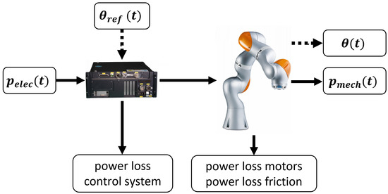
Figure 5.
Energy flow through the robot system [3]. The target variable for modeling is the electrical power supplied .
Portions of the total power supplied are lost due to losses in the control system, losses in the motors, as well as losses through friction. What remains is the mechanical power that can be used for performing various tasks.
As already shown in Section 2.4, the mechanical power is closely related to the electrical power and can be calculated by (). In robotics, the torque acting on a robot axis can be calculated by solving the so-called inverse dynamics problem, which is given as a set of nonlinear differential equations in the variables angle , angular velocity , and angular acceleration [23].
where is a symmetric, positively defined mass matrix, and are forces that combine centripetal, coriolis, gravitational, and frictional terms. By multiplying (3) with , the mechanical power of the system under consideration is given by a nonlinear function with the variables angle , angular velocity , and angular acceleration . Since the electrical power is closely related to the mechanical power, and the mechanical power depends substantially on the three variables: , , and . These variables can be considered as suitable features to model the system behavior via machine learning algorithms.
For extraction of the engineered features, the first- and second-order finite difference method is applied to the recorded data ((2) and (4)).
Before the collected data is handed over to the selected modeling algorithms, normalization is performed. For the electrical power, normalization is chosen with , with power normalization parameters are chosen with and .Angle, angular velocity, and angular acceleration are scaled by the factors , , and .
3.2. Models
Three different distinct model architectures were developed, namely dense models, LSTM models, and LSTM models with convolutional layers, as can be seen in Figure 6. Both the dense and LSTM models can take a variable amount of input features. One network has only the normalized seven axis angles as input, the second additionally has the normalized angular velocities as input, which leads to a 14-dimensional input, and the third network has all 21 constructed features as input.
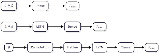
Figure 6.
Architectures of the models developed ranging from the least to the most complex. From top to bottom: dense architecture, LSTM architecture, and LSTM with convolutional layer architecture.
The dense models consist of four linear layers with a ReLU activation function. It accepts features in the format , where b is the batch size, and f is the number of features for one timestamp. The LSTM network structure consists of a sequence input layer, followed by an LSTM layer with 10 hidden units, succeeded by a four-layered dense network without activation functions. The last layer is a one-dimensional output layer. It accepts features in the format , where b is the batch size, t is the timestamps, and f is the individual features. With this structure, three networks were set up that differ only in their input dimension. Importantly, the datasets used for LSTM and dense models are identical, only the input arrays are reshaped to match the required format of each architecture before training and evaluation.
LSTM with convolutional layer for feature extraction is a model structure that is capable of automatically extracting features from the data without requiring any prior knowledge of the system. It is interesting to note that the derivative of a signal can be computed by convolution of the signal with an appropriate filter kernel. Common filter kernels are therefore the first- and second-order derivative of a Gaussian g(t) ((5) and (6)) [24].
When the width of the kernels is reduced to L = 3, then the convolution of the resulting kernels with a signal is the same as the calculation of the first and second finite differences given by (2) and (4) for . Hence, a convolutional layer with multiple filter kernels of width 3 prior to the LSTM layer can, in principle, provide the same performance as the networks with manually extracted features. For this architecture, the input features are arranged in the format , where b is batch size, f is the individual features, and L corresponds to the kernel width. The datasets remain the same but are reshaped so that the CNN consistently receives L timestamps, with appropriate padding applied at the sequence boundaries.
The tested network structures are LSTM, dense, and LSTM with preceding convolutional layers. Shown in Table 1 are the tested structures and their number of parameters for complexity comparison.

Table 1.
Number of parameters for each model [3].
We use LSTM (lstm-) and dense (mlp-) networks with different input features. We either use only the angular values (-Nf7), angular values and angular velocity (-Nf14), or all (-Nf21) as input to the neural nets. For dense versions, small architectures (-small) with similar numbers of parameters as compared to the LSTMs as well as architectures with higher parameter numbers (-large) were assessed. For LSTM with convolutional layer (cnn-), we trained two networks with three kernels (-k3) and a varying kernel width of (-L3) and (-L5). This configuration only expects the angular values . For model training and evaluation, the datasets were split into training, testing, and validation sets. When splitting, we ensured that no recordings based on the same source trajectory were found in the same split. All models were trained using Adam optimizer [25].
4. Privacy-Preserving Collaborative Energy Prediction
To address the challenges related to disclosing sensitive information, we introduce a ppML framework that utilizes SMPC techniques for energy modeling. This framework ensures that
- Model providers maintain the confidentiality of their trained energy models.
- Clients can perform encrypted inference on proprietary trajectories without exposing sensitive data.
SMPC can be computationally intensive. In scenarios where real-time or near real-time performance is required—such as energy optimization—slow computation can be a limiting factor for certain approaches. It is important to note that the computations performed by the adopted methodology are accurate up to floating-point rounding errors. As a result, the prediction accuracy of the underlying networks remains unaffected.
To ensure that the performance requirements of our use case are satisfied, we evaluate three state-of-the-art secure multi-party computation (SMPC) frameworks: MP-SPDZ [16], CrypTen [21], and SecretFlow-SPU [17]. For improved reproducibility, two well-established and widely adopted neural network architectures—AlexNet [26] and LeNet [27]—were used. Inference was conducted using SMPC following a clear-text training phase. It is important to note that training neural network models in the encrypted domain was not feasible due to performance limitations. As shown in Table 2, SecretFlow-SPU achieved the lowest inference time per sample. Combined with its user-friendly interface and ease of implementation, SecretFlow-SPU was chosen as the primary framework for this work.
Table 2.
Comparison of the inference times of several SMPC frameworks on two open-source models. The times shown are for single sample inference [3].
4.1. Overview of SPU
For privacy-preserving inference, the SecretFlow-SPU framework [17] was employed. The architecture of the SPU framework is illustrated in Figure 7. Unlike other frameworks such as CrypTen [21] and MP-SPDZ [16], SPU can integrate machine learning models from any popular framework that can be compiled to the higher level operations (HLO) intermediate representation, requiring only minimal modifications to the training and inference scripts. The SPU frontend processes this HLO representation and transforms it into a SPU-specific PPHLO representation, where additional MPC-specific optimizations and data visibility annotations are applied. This representation is then passed to the SPU backend, which operates across multiple nodes based on the underlying MPC protocol. SPU follows the single-program-multiple-data (SPMD) model, meaning all nodes receive and execute the same code.
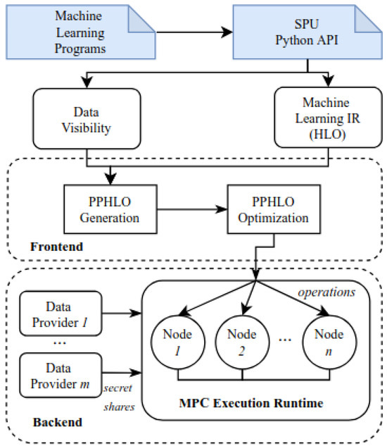
Figure 7.
Overview of SPU architecture [17]. For machine learning development the main interaction is with SPU Python API.
4.2. Problems ppML
The major obstacle that ppML using SMPC presents is the increased computational and communication overhead required for the computing nodes. This is illustrated in Table 3, where a noticeable difference between inference of plaintext models and SMPC models can be observed. Coupled with other real-world factors like network latency and packet loss, a faster inference speed for SMPC is required in order to achieve real-world adoption. Several optimization strategies have been proposed and evaluated in the past [28,29,30]. However, these are mostly used for large language models (LLMs), and their effect on smaller networks similar to the ones we have developed is untested. Two such optimizations are evaluated in this paper, namely enabling plaintext weights through model permutation and evaluating activation functions in plaintext.
Table 3.
Comparison of plaintext vs. SMPC inference times.
Typically, SPU or other popular SMPC frameworks view neural network inference as a function of two inputs, those being the input features (robots angles and their derivations in this case) and trained model weights. A typical inference in SPU secret shares both of those inputs, making them illegible for honest-but-curious adversaries. While this approach is secure for both inputs, it suffers from larger computational overhead and therefore larger inference times, making it harder to apply for real-life applications. One way to speed up the inference is to make one of the inputs public. In the case of open-source models, the biggest candidates are the pre-trained model parameters. To still ensure a secure model inference, linear layer parameters and input features can be permuted using predetermined random permutation matrices [28]. This way linear layers can be kept public, and the input features will be used in their permuted secret-shared state. This has the potential to drastically reduce inference times for fully connected linear layers without sacrificing too much of the security.
Another way of possibly reducing model inference times in SMPC is to evaluate the activation functions in plaintext. Activation functions in SMPC inference take, contrary to the plaintext inference, the majority of the inference time [29]. Different activation functions have different impacts on inference times and there has been an effort to minimize this added overhead by simplifying the activation functions. In the case of our developed networks, ReLU activation is used. This belongs to the class of already very simple functions, and further reducing it would introduce a significant error to the utility of the network. Therefore, a different approach was chosen to investigate, which is the evaluation of activations in plaintext. The secret-shared intermediary values can be sent to and reconstructed by the data owner, who then performs the activation locally in plaintext and again secret-shares the resulting values to the nodes. This process is repeated until all activations in the network have been evaluated.
5. Evaluation Results
In this section, all our developed models are evaluated. First, the qualitative results of the models are discussed purely in plaintext form. Second, the inference times of the models are discussed in SMPC form. As the quality of the models does not change compared to plaintext, only inference time is taken into consideration as the main metric. Third, the impact of the two proposed optimization strategies is discussed on the best-performing model. Finally, the deployment considerations for SMPC models are evaluated, and the impact of network delay and packet loss is analyzed.
5.1. Models’ Quality Evaluation
The trained models are evaluated using the metrics mean absolute error (MAE), root mean squared error (RMSE). and mean absolute percentage error (MAPE) given the following equations:
Metrics computed from the combined LimSp and AllSp datasets are shown in Table 4. The results indicate that the manually engineered features are informative. Using the complete set of , , and features (-Nf21) resulted in the lowest error rates. In contrast, models without CNN layers and trained solely on seven axis angles (-Nf7) showed the weakest performance. Although the MAE for convolutional models is slightly higher compared to models using all three input feature types (-Nf21), the difference remains within a comparable range. Notably, LSTM networks outperform fully connected models when only or are used as inputs. However, when all features are included, fully connected models achieve better performance. Furthermore, the number of weights in the dense models does not appear to have a significant impact on performance, as the metrics remain stable across different configurations.
Table 4.
Comparison of metrics for tested model structures. Values are calculated from the combined LimSp and AllSp datasets [3].
To assess the impact of different datasets on model performance, metrics were computed separately for the LimSp and AllSp datasets. Table 5 summarizes the results, with mean absolute error (MAE) used as the primary evaluation metric. The results show that performance is notably better on the LimSp dataset. This outcome is expected, as the AllSp dataset covers a much larger configuration space, which in turn requires a substantially greater number of samples for comparable performance.
Table 5.
Comparison of mean absolute error for tested model structures. Values are calculated from the combined LimSp and AllSp datasets [3].
The difference in performance is depicted in Figure 8, which shows predictions for selected sequences from selected model mlpNf21-large. The sequences illustrate the worst predictions according to the MAE value for the LimSp and AllSp datasets, respectively.
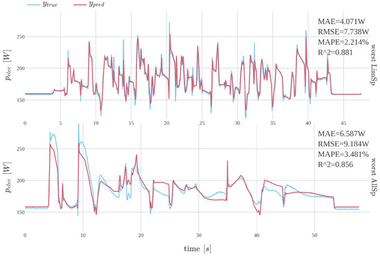
Figure 8.
Comparison of the worst predictions on LimSp and AllSp datasets with respect to MAE using model mlpNf21-large.
The results indicate that the model performs effectively on the LimSp dataset, with predictions closely matching the measured values—even for the lowest-performing sequences. In contrast, the AllSp dataset reveals discrepancies in certain parts of the sequences, suggesting that model performance may be limited by the relatively small number of available training samples. Overall, these findings support the feasibility of using a data-driven approach with neural networks for energy prediction modeling.
5.2. Models Evaluation Under SMPC
The trained models are evaluated using inference time under SMPC and inference time in plaintext form. All the benchmarks were established on an Intel Xeon W-2245 CPU, 126 GB of RAM using Ubuntu 24.04 and Python 3.10.14. The SMPC protocol chosen was ABY3 with three computing nodes and two provider nodes, one providing the inputs and the other one providing the trained model weights. All tests were conducted within a local area network. Table 6 presents the performance measurements for SecretFlow-SPU using the developed energy prediction networks. The results highlight the following observations:
Table 6.
Comparison of inference time for all models in both SMPC and plaintext form. For SMPC inference both model weights and inputs are secret shared [3].
- Feature dimensionality has minimal impact on inference performance in the encrypted domain.
- The type of network layers (recurrent, convolutional, or dense) plays the most significant role in determining performance when used with SPU.
Convolutional networks exhibit increased computational demands in the encrypted domain. In contrast, dense architectures, which require fewer operations, are particularly well-suited for SMPC environments. Recurrent networks such as LSTMs, while composed of relatively simple operations, are less amenable to parallelization due to their sequential computation of hidden and cell states.
5.3. Analyzing Performance-Privacy Trade-Off
The impact of the two optimization strategies mentioned in the previous chapter on the encrypted inference time was studied as well. The results can be seen on Table 7. The model chosen is the MLP 21 due to its best performance in both inference time and qualitative results and due to its simple architecture, which made experimentation easier.
Table 7.
Impact of different optimization attempts on mlpNf21-large. Time encrypted shows how the optimization affects the SMPC inference. For permutation of weights this shows the impact of keeping the model weights public and permuted, while the inputs are permuted and secret-shared.
For the first strategy of evaluating activation functions in plaintext form, slightly worse inference time was measured. This could be because the time required for collecting shares, reconstructing them, and then again resharing the outputs multiple times during forward pass is more computationally expensive than just a simple evaluation of the function in SMPC form. This optimization can prove useful for more complex neural networks with more complicated and less frequent activations and is subject to further study.
The second strategy of permuting both the weights and inputs, while keeping the weights in plaintext form, proved to be a significant speed increase resulting in a 2.4-times inference time decrease compared to a full encrypted MLP 21 inference. This is an expected outcome, as computing on one less encrypted output significantly reduces the computational overhead.
5.4. Deployment Considerations
The impact of network delay and packet loss on the inference has also been studied, as these metrics are an important factor to consider [31], especially when talking about SMPC inference, as it relies heavily on inter-node communication for some operations. As can be seen on Figure 9, the effect of network delay linearly increases the inference time for all models, but the LSTM and LSTM with convolution have much steeper slopes and are therefore more affected. From the figure, it can also be seen that both LSTM and LSTM with convolution have almost the same increase, which hints at the fact that the LSTM layer affects this metric the most. Similarly for packet loss, the relationship seems to be almost linear, with some visible nonlinearities occurring with higher packet loss, especially for models using LSTM layers. However, scenarios involving very high packet loss are not the primary focus of this work, as they reflect severe communication issues rather than typical real-world conditions.
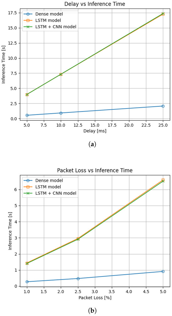
Figure 9.
Effects of network complications on inference time: (a) effect of added network delay; (b) effect of added packet loss. Note that both models using LSTM layer have almost identical inference times under these conditions and are therefore overlapping in the graphs.
6. Integration into MLOps
Machine learning operations (MLOps) are a set of best practices for experimenting, developing, deploying, and monitoring of machine learning (ML) systems in an end-to-end manner. Bringing the ML system to production involves several steps shown in Figure 10.
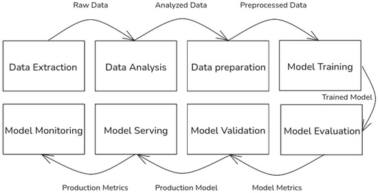
Figure 10.
Data science steps required for the development of a machine learning system.
The amount of automation of these steps dictates the level of maturity of the ML system (https://cloud.google.com/architecture/mlops-continuous-delivery-and-automation-pipelines-in-machine-learning (accessed on 30 June 2025)). When it comes to impact of privacy-preserving machine learning inference on these steps, especially the final two steps, model serving and model monitoring are most affected.
6.1. MLOps Workflow
An example of an MLOps workflow can be seen in Figure 11. One of the key differences between MLOps workflows and non-MLOps workflows is the development target. In non-MLOps workflows, a trained and validated model is deployed to production and served for inference. In MLOps workflows an automated pipeline that conducts the data processing, model training, and evaluation is deployed to production. This pipeline, if the resulting model is deemed ready for production, pushes the model to a model registry, which serves as a centralized repository for model structure and artifacts. From here the model-serving service takes the latest, best model and conducts prediction service. The prediction service is then monitored and acts as a trigger to initiate the deployed pipeline again if the model’s performance degrades under a certain threshold.
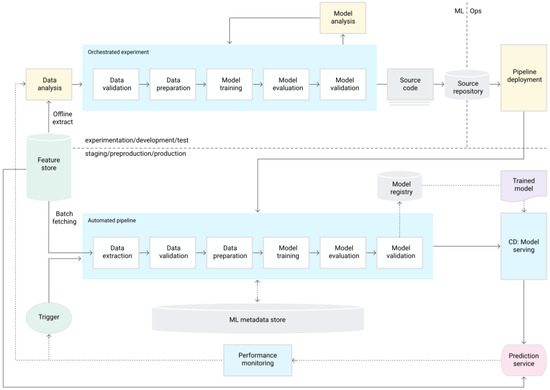
Figure 11.
Example of an MLOps workflow. Taken from [32].
6.2. Towards a ppMLOps Workflow
To integrate ppML into the existing approach, the following extensions would be required, as encountered in our experiments:
Model serving is a process where the validated model that is being promoted to production is being served to be used for inference by the end user. Services that provide this process are typically cloud providers (Amazon AWS, Microsoft Azure, Google Cloud, etc.). In the context of ppML, the inference process generally involves three parties:
- The model owner, who provides the model structure as well as the trained parameters of the latest validated model,
- The end user, who provides private data for inference, and
- The SMPC inference service, which processes inputs from the other two parties and returns the result to the End User.
Among these, the SMPC service bears the majority of the complexity. The developers of this service should abstract the SMPC process enough so that it behaves like a singular virtual machine from the perspective of both the model owner and the end user. Once this abstraction is developed and standardized, model serving will be similar to that of traditional MLOps pipelines, since the underlying privacy-preserving operations are abstracted and no longer interfere with the deployment process.
Model monitoring is a process that provides data about the quality of the model being used in production. This data can then be potentially used as a trigger to retrain/redevelop the model, as models are inherently decaying over time due to the availability of new data or shifting of the trends in data.If the model inference is to be run with SMPC, then this step is impossible to complete, as the result of the inference should only be visible to the end user. A solution to this could be monitoring of a copy of the model conducted within the domain of the model owner.
The final part that needs to be addressed regarding the MLOps pipeline as well as machine learning model design is the actual model architecture and the experimental phase of model development. In the previous chapter, it was shown that even with a much simpler model structure similar or even better qualitative results can be achieved, while having the lowest inference times. The simpler architecture has even more impact on ppML, as the inference time in the encrypted domain has become a critical metric to keep track of. Machine learning experts should strive for simplicity and very specifically designed models for the problem they address if optimal performance in the encrypted domain is to be achieved.
7. Conclusions
Our findings demonstrate that a purely data-driven learning approach achieves competitive accuracy in predicting energy consumption, particularly when using manually engineered features such as joint angles, velocities, and accelerations. Among the evaluated model architectures, dense networks that used all available features delivered the best results in terms of qualitative metrics and inference speed, both in plaintext and encrypted settings.
We further integrated privacy-preserving machine learning (ppML) techniques based on secure multi-party computation (SMPC) to enable secure inference on proprietary data without revealing either the input or the trained model weights. Our analysis revealed that model architecture significantly affects inference performance in the encrypted domain, with dense networks being more efficient than convolutional or recurrent architectures. We also evaluated optimization strategies such as plaintext weight permutation and plaintext activation evaluations, showing that plaintext weight permutation can significantly reduce inference times but with trade-offs in privacy.
Furthermore, we examined the implications of ppML integration within modern machine learning operations (MLOps) workflows. Most MLOps stages remain unaffected, but our analysis identified two areas, namely model serving and model monitoring, that require some adaptations. More specifically, serving privacy-preserving models demands careful coordination between model owners, end-users, and secure computation services, while traditional monitoring must be redesigned since model outputs are not directly observable under SMPC.
This work provides a framework for secure, data-driven energy prediction in industrial robotics. It contributes insights for both the design of efficient ppML models and the adaptation of MLOps pipelines, supporting adoption of ppML in increasingly complex industrial ecosystems.
Future work might focus on developing and evaluating more complex modeling tasks in industrial settings (different robot configurations, effect of a loaded arm on the model, etc.), potentially giving more insights on ppML for a different set of machine learning architectures. It would be also interesting to streamline the performance evaluation process, be it by researching novel means to support software developers, by estimating expected performance for given models, or by providing automated guidance for optimization. Another focus might be deploying and testing our framework in a live setting and evaluating it with realistic network complications. Investigating the potential integration of industrial standards for communication (e.g., OPC UA) into the ppML pipeline is another potential extension in the future.
Author Contributions
Conceptualization, P.S., A.S., T.L., S.H. and R.H.; methodology, P.S., A.S., T.L., S.H. and R.H.; software, A.S. and P.S.; validation, A.S. and P.S.; formal analysis, P.S.; investigation, A.S. and P.S.; data curation, P.S.; writing—original draft preparation, A.S. and P.S.; writing—review and editing, A.S., P.S., T.L., S.H. and R.H.; visualization, A.S. and P.S.; supervision, T.L., S.H. and R.H.; All authors have read and agreed to the published version of the manuscript.
Funding
This work has received funding from the EU Horizon Europe Work Programme under project QSNP (no. 101114043) and the Austrian Research Promotion Agency FFG within the PRESENT project (grant no. 899544).
Institutional Review Board Statement
Not applicable.
Data Availability Statement
Dataset available on request from the authors.
Conflicts of Interest
The authors declare no conflicts of interest.
References
- Abdoune, F.; Ragazzini, L.; Nouiri, M.; Negri, E.; Cardin, O. Toward Digital Twin for Sustainable Manufacturing: A Data-Driven Approach for Energy Consumption Behavior Model Generation. Comput. Ind. 2023, 150, 103949. [Google Scholar] [CrossRef]
- Sekala, A.; Blaszczyk, T.; Foit, K.; Kost, G. Selected Issues, Methods, and Trends in the Energy Consumption of Industrial Robots. Energies 2024, 17, 641. [Google Scholar] [CrossRef]
- Steurer, P.; Skuta, A.; Hegenbart, S.; Hoch, R.; Loruenser, T. Data-Driven Modeling for Privacy-Preserving Energy Prediction of Industrial Robots. In Proceedings of the 5th Winter IFSA Conference on Automation, Robotics & Communications for Industry 4.0/5.0, ARCI’ 2025, Granada, Spain, 19–21 February 2025; Yurish, S., Ed.; pp. 184–189. [Google Scholar] [CrossRef]
- Walther, J.; Weigold, M. A Systematic Review on Predicting and Forecasting the Electrical Energy Consumption in the Manufacturing Industry. Energies 2021, 14, 968. [Google Scholar] [CrossRef]
- Liu, A.; Liu, H.; Yao, B.; Xu, W.; Yang, M. Energy consumption modeling of industrial robot based on simulated power data and parameter identification. Adv. Mech. Eng. 2018, 10, 1687814018773852. [Google Scholar] [CrossRef]
- Yan, K.; Xu, W.; Yao, B.; Zhou, Z.; Pham, D.T. Digital Twin-Based Energy Modeling of Industrial Robots. In Methods and Applications for Modeling and Simulation of Complex Systems, Proceedings of the 18th Asia Simulation Conference, AsiaSim 2018, Kyoto, Japan, 27–29 October 2018; Communications in Computer and Information Science. Li, L., Hasegawa, K., Tanaka, S., Eds.; Springer: Singapore, 2018; pp. 333–348. [Google Scholar] [CrossRef]
- Kajzr, D.; Myslivec, T.; Černohorský, J. Modelling, Analysis and Comparison of Robot Energy Consumption for Three-Dimensional Concrete Printing Technology. Robotics 2024, 13, 78. [Google Scholar] [CrossRef]
- Swevers, J.; Verdonck, W.; De Schutter, J. Dynamic Model Identification for Industrial Robots. IEEE Control Syst. Mag. 2007, 27, 58–71. [Google Scholar] [CrossRef]
- Wu, J.; Wang, J.; You, Z. An overview of dynamic parameter identification of robots. Robot. Comput.-Integr. Manuf. 2010, 26, 414–419. [Google Scholar] [CrossRef]
- Bargsten, V.; Zometa, P.; Findeisen, R. Modeling, parameter identification and model-based control of a lightweight robotic manipulator. In Proceedings of the 2013 IEEE International Conference on Control Applications (CCA), Hyderabad, India, 28–30 August 2013; pp. 134–139, ISSN 1085-1992. [Google Scholar] [CrossRef]
- Paryanto; Brossog, M.; Bornschlegl, M.; Franke, J. Reducing the energy consumption of industrial robots in manufacturing systems. Int. J. Adv. Manuf. Technol. 2015, 78, 1315–1328. [Google Scholar] [CrossRef]
- Zhang, M.; Yan, J. A data-driven method for optimizing the energy consumption of industrial robots. J. Clean. Prod. 2021, 285, 124862. [Google Scholar] [CrossRef]
- Yin, S.; Ji, W.; Wang, L. A machine learning based energy efficient trajectory planning approach for industrial robots. Procedia CIRP 2019, 81, 429–434. [Google Scholar] [CrossRef]
- Lorünser, T.; Wohner, F.; Krenn, S. A Privacy-Preserving Auction Platform with Public Verifiability for Smart Manufacturing. In Proceedings of the ICISSP 2022, Online, 9–11 February 2022; Mori, P., Lenzini, G., Furnell, S., Eds.; SCITEPRESS: Setúbal, Portugal, 2022; pp. 637–647. [Google Scholar] [CrossRef]
- Lorünser, T.; Wohner, F.; Krenn, S. A Verifiable Multiparty Computation Solver for the Linear Assignment Problem: And Applications to Air Traffic Management. In Proceedings of the CCSW 2022, Los Angeles, CA, USA, 7–11 November 2022; Regazzoni, F., van Dijk, M., Eds.; ACM: New York, NY, USA, 2022; pp. 41–51. [Google Scholar] [CrossRef]
- Keller, M. MP-SPDZ: A Versatile Framework for Multi-Party Computation. In Proceedings of the 2020 ACM SIGSAC Conference on Computer and Communications Security, Virtual, 9–13 November 2020. [Google Scholar]
- Ma, J.; Zheng, Y.; Feng, J.; Zhao, D.; Wu, H.; Fang, W.; Tan, J.; Yu, C.; Zhang, B.; Wang, L. SecretFlow-SPU: A Performant and User-Friendly Framework for Privacy-Preserving Machine Learning. In Proceedings of the USENIX ATC ’23, Boston, MA, USA, 10–12 July 2023; pp. 17–33. [Google Scholar]
- Mohassel, P.; Rindal, P. ABY3: A Mixed Protocol Framework for Machine Learning. In Proceedings of the 2018 ACM SIGSAC CCS, CCS ’18, Toronto, ON, Canada, 15–19 October 2018; pp. 35–52. [Google Scholar] [CrossRef]
- Cramer, R.; Damgård, I.; Escudero, D.; Scholl, P.; Xing, C. SPD2k: Efficient MPC mod 2k for Dishonest Majority. In Advances in Cryptology – CRYPTO 2018, Proceedings of the 38th Annual International Cryptology Conference, Santa Barbara, CA, USA, August 19–23, 2018; Springer: Berlin/Heidelberg, Germany, 2018; Volume II, pp. 769–798. [Google Scholar] [CrossRef]
- Huang, Z.; Lu, W.j.; Hong, C.; Ding, J. Cheetah: Lean and Fast Secure Two-Party Deep Neural Network Inference. In Proceedings of the 31st USENIX Security Symposium (USENIX Security 22), Boston, MA, USA, 10–12 August 2022. [Google Scholar]
- Knott, B.; Venkataraman, S.; Hannun, A.; Sengupta, S.; Ibrahim, M.; van der Maaten, L. CrypTen: Secure Multi-Party Computation Meets Machine Learning. In Proceedings of the Advances in Neural Information Processing Systems 34 (NeurIPS 2021), Online, 6–14 December 2021. [Google Scholar]
- Pub MA KUKA Sunrise Cabinet (PDF) en. Available online: https://www.oir.caltech.edu/twiki_oir/pub/Palomar/ZTF/KUKARoboticArmMaterial/MA_KUKA_Sunrise_Cabinet_en.pdf (accessed on 27 August 2025).
- Lynch, K.M.; Park, F.C. Modern Robotics: Mechanics, Planning, and Control; Cambridge University Press: Cambridge, UK, 2017. [Google Scholar]
- Birchfield, S. Image Processing and Analysis, 1st ed.; Cengage Learning: Mason, OH, USA, 2016. [Google Scholar]
- Kingma, D.P.; Ba, J. Adam: A Method for Stochastic Optimization. In Proceedings of the 3rd International Conference on Learning Representations, ICLR 2015, San Diego, CA, USA, 7–9 May 2015; Conference Track Proceedings. Bengio, Y., LeCun, Y., Eds.; 2015. [Google Scholar]
- Krizhevsky, A.; Sutskever, I.; Hinton, G.E. ImageNet Classification with Deep Convolutional Neural Networks. In Proceedings of the Advances in Neural Information Processing Systems 25 (NIPS 2012), Lake Tahoe, NV, USA, 3–6 December 2012; Pereira, F., Burges, C., Bottou, L., Weinberger, K., Eds.; Curran Associates, Inc.: Red Hook, NY, USA, 2012; Volume 25. [Google Scholar]
- Lecun, Y.; Bottou, L.; Bengio, Y.; Haffner, P. Gradient-based learning applied to document recognition. Proc. IEEE 1998, 86, 2278–2324. [Google Scholar] [CrossRef]
- Luo, J.; Chen, G.; Zhang, Y.; Liu, S.; Wang, H.; Yu, Y.; Zhou, X.; Qi, Y.; Xu, Z. Centaur: Bridging the Impossible Trinity of Privacy, Efficiency, and Performance in Privacy-Preserving Transformer Inference. arXiv 2024, arXiv:2412.10652. [Google Scholar] [CrossRef]
- Luo, J.; Zhang, Y.; Zhang, Z.; Zhang, J.; Mu, X.; Wang, H.; Yu, Y.; Xu, Z. SecFormer: Fast and Accurate Privacy-Preserving Inference for Transformer Models via SMPC. arXiv 2024, arXiv:2401.00793. [Google Scholar] [CrossRef]
- Li, D.; Shao, R.; Wang, H.; Guo, H.; Xing, E.P.; Zhang, H. MPCFormer: Fast, performant and private Transformer inference with MPC. arXiv 2023, arXiv:2211.01452. [Google Scholar] [CrossRef]
- Lorünser, T.; Wohner, F. Performance Comparison of Two Generic MPC-frameworks with Symmetric Ciphers. In Proceedings of the ICETE (2), Paris, France, 8–10 July 2020; pp. 587–594. [Google Scholar]
- Google MLOps Archtecture. Available online: https://cloud.google.com/architecture/mlops-continuous-delivery-and-automation-pipelines-in-machine-learning (accessed on 1 July 2025).


Disclaimer/Publisher’s Note: The statements, opinions and data contained in all publications are solely those of the individual author(s) and contributor(s) and not of MDPI and/or the editor(s). MDPI and/or the editor(s) disclaim responsibility for any injury to people or property resulting from any ideas, methods, instructions or products referred to in the content. |
© 2025 by the authors. Licensee MDPI, Basel, Switzerland. This article is an open access article distributed under the terms and conditions of the Creative Commons Attribution (CC BY) license (https://creativecommons.org/licenses/by/4.0/).