A Novel Adaptive and Nonlinear Electrohydraulic Active Suspension Control System with Zero Dynamic Tire Liftoff

Abstract

In this paper, a novel adaptive control system (NAC) is proposed for a restricted quarter-car electrohydraulic active suspension system. The main contribution of this NAC is its explicit tackling of the trade-off between passenger comfort/road holding and passenger comfort/suspension travel. Reducing suspension travel oscillations is another control target that was considered. Many researchers have developed control laws for constrained active suspension systems. However, most of the studies in the works of the latter have not directly examined the compromise between road holding, suspension travel, and passenger comfort. In this study, we proposed a novel adaptive control system to explicitly address the trade-off between passenger comfort and road holding, as well as the compromise between passenger comfort and suspension travel limits. The novelty of our control technique lies in its introduction of a modeling system for a dynamic landing tire system aimed at avoiding a dynamic tire liftoff. The proposed control consists of an adaptive neural networks’ backstepping control, coupled with a nonlinear control filter system aimed at tracking the output position of the nonlinear filter. The tracking control position is the difference between the sprung mass position and the output nonlinear filter signal. The results indicate that the novel adaptive control (NAC) can achieve the handling of car–road stability, ride comfort, and safe suspension travel compared to that of the other studies, demonstrating the controller’s effectiveness.

1. Introduction

A vehicle active suspension is a mechanical vibration system. The active suspension aims primarily to minimize the transmission of vertical road forces to the sprung mass (passenger comfort) and to maximize tire–road contact (road holding) [1]. An active suspension system must operate within safe travel ranges to avoid exceeding the suspension travel limits. Consequently, the hydraulic actuator of the active suspension generates vertical forces to enable a compromise between ride comfort, suspension deflection, and road holding. To ensure passenger comfort, the hydraulic actuator can absorb the road energy transmitted to the sprung mass. Further, the actuator can generate vertical forces to improve car stability and safety. Although the active suspension is an important system in the vehicle structure, it must deal with several challenges. For example, the system has several inherent undesirable dynamic characteristics, such as nonlinear dynamics, parametric uncertainties, and external perturbations [2]. Moreover, it forces a trade-off between passenger comfort, road holding, and limited suspension travels.

Many control strategies have been applied in vehicle systems, which have multiple modeling systems. A high-precision hydraulic pressure control based on linear pressure drop modulation in valve critical equilibrium state was developed in [3]. The control methodology in that study was a sliding mode control based on high-precision hydraulic pressure for an automobile brake system. The experimental tests and validation system showed improvements in the control performance and robustness. In [4], a dynamic state estimation for the advance brake system of an electric vehicle was implemented by using deep recurrent neural networks. In that study, an integrated time series model based on multivariate deep recurrent neural networks with long short-term memory units was applied for brake pressure estimation of the electric vehicle system. The test results showed the effectiveness of the proposed integrated method. In [5], a neuro-fuzzy adaptive control for a full car nonlinear active suspension with onboard antilock braking system was investigated. A comparative study was done between the intelligent control system and passive suspension. The method showed an improvement in control performance.

The vehicle active suspension system is among the systems that have been most studied in recent years. Active suspensions in vehicles serve mainly to isolate the car cabin from road perturbations and provide vehicle handling under different operating conditions. Many researchers have developed control strategies for these systems. Testing and simulation of a motor vehicle suspension were carried out in [6]. In the study, experiments were done by applying impulse road input perturbation. The results showed reduction of transmitted road energy to the system. Road profiles on a rig for indoor vehicle chassis and suspension durability testing were reproduced in [7]. An impulse road input was applied in the test rig. The results showed control performance improvements. Other studies have been developed for the active suspension system in a bed to overcome the dynamic nonlinearities and parametric uncertainties present. In [8], a sliding mode and fuzzy hybrid control system were developed to overcome dynamic nonlinearities and reduce control chattering for a quarter-car active suspension. There, a fuzzy hybrid control system was designed to track a force and a position and reduce the control chattering. The controller provided control performance improvements. On the other hand, the road holding and the suspension travel limits were not addressed.

Many researchers have also developed control strategies for active suspension systems. For example, in [9], an adaptive tracking control was developed to overcome the dynamic nonlinearities for a non-ideal actuator of a quarter-car active suspension. The actuator’s nonlinearities of both dead-zone and hysteresis were addressed in that study. The experimental results showed a better balance between isolation performance and energy consumption for the active suspension. Even though several road case designs were applied, road holding was not clearly indicated in results. An adaptive neural networks’ control system was designed by [10]. In that study, the road design could not generate the tire liftoff phenomenon to indicate road holding. In [11], a backstepping control law was investigated to monitor suspension travel by using a nonlinear control filter. The results showed an improvement in control performance. However, road holding was not addressed. A multi-objective control system for a constrained active suspension, designed based on both barrier and quadratic Lyapunov functions, was developed in [12], with results showing control performance improvements. However, the system did not address tire liftoff phenomenon. In [13], an adaptive control was developed for nonlinear active suspension. While the system provided suspension deflection and road holding, its bumpy road design did not address tire liftoff either. In [14], an adaptive backstepping-based tracking controller was investigated for nonlinear half-active suspension. In that study, zero dynamics system was applied to ensure that all dynamic order errors were bounded. Although the results showed improvements in control performance, tire liftoff was not tested. In [15], an adaptive backstepping tracking control was developed for an uncertain nonlinear active suspension. The control consisted of a model-reference control combined with coordinated adaptive backstepping control systems. Simulation results showed control performance degradation and, once again, tire liftoff was not examined. In [16], a linear disturbance observer coupled with a sliding mode scheme was developed for an active suspension with a non-ideal actuator. The results showed compensation improvements despite the presence of a dead-zone and hysteresis, as well as modeling uncertainty. In this case as well, the tire liftoff effect was not considered. In [17], an adaptive neural networks’ control was developed for a restricted quarter-car active suspension. Both the barrier Lyapunov function and zero dynamics system were applied to prevent any violation of the system’s constraints. There was an improvement in the control performance, but the tire liftoff was not evaluated.

As we can see, while previous works showed improvements in control performance, they universally did not examine tire liftoff. Therefore, the results in previous studies cannot indicate road-holding robustness.

In general, high-frequency bumpy road input can generate tire liftoff phenomenon. Thus, road holding can clearly be addressed. In [18], an approximation-free control was developed for quarter-car active suspension. In that study, both a random road and a high-frequency bumpy road designs were examined. The results showed an improvement in road holding when the random road design was applied. Even though previous studies were developed, improving in control performance, the researchers did not explicitly address both a trade-off between ride comfort and road holding, and a trade-off between ride comfort and suspension travel limits.

In this study, a novel control system was developed to handle the inherent trade-off between passenger comfort/road holding, passenger comfort/suspension contraction limitation, and passenger comfort/suspension expansion limitation, as well as to overcome the dynamic nonlinearities and parametric uncertainties of quarter-car active suspension systems. The novelty of this study lies in its aim, which is two-fold. On the one hand, it aimed to overcome and prevent the dynamic tire liftoff phenomenon by implementing a new model of a dynamic landing tire system. On the other hand, it aimed to avoid exceeding suspension travel limits. We broke down the suspension deflection into two different suspension travel limits, namely, suspension contraction limitation and suspension expansion limitation. We then redesigned a nonlinear control filter that was introduced in [11]. The redesigned filter became three regions, which are a dead zone, a dynamic landing tire nonlinear function, and a suspension deflection nonlinear function. This design of the nonlinear control filter can accommodate and improve the trade-off between passenger comfort, road holding, and suspension travel. Therefore, the novel adaptive control system ‘NAC’ system is an adaptive neural networks’ backstepping control system coupled with the nonlinear control filter. The adaptive neural networks’ control system can deal with unknown smooth functions of the modeling system. The summarized contributions of this article are:

• The NAC was established to achieve passenger comfort while keeping road holding and prevention of exceeding suspension travel limits.
• The NAC was also designed to reduce suspension travel oscillations.
• A dynamic landing tire modeling system was developed to evaluate a required tire vertical displacement, which maintains road holding for the car.
• The suspension travel limits were separately chosen to be suspension contraction limitation and suspension expansion limitation in order to realize operation conditions.
• In NAC structure, the adaptive radial basis function neural networks were designed to approximate nonlinear and unknown bounding functions in the modeling system.

Finally, simulation examples demonstrated the performance of the NAC in enhancing passenger comfort, maintaining road holding, avoiding reaching suspension travel limits, and reducing suspension travel oscillation.

The rest of the paper is broken down as follows. Section 2 presents the notations used and the problem statement. Section 3 describes the control law design, which includes the nonlinear control filter, the adaptive neural networks’ backstepping control design, and zero dynamics system. Section 4 discusses the illustrated example of a comparative study of a filtered active suspension, an unfiltered active suspension, and a passive suspension. Section 5 presents the conclusion and future works.

2. Notation and Problem Statement

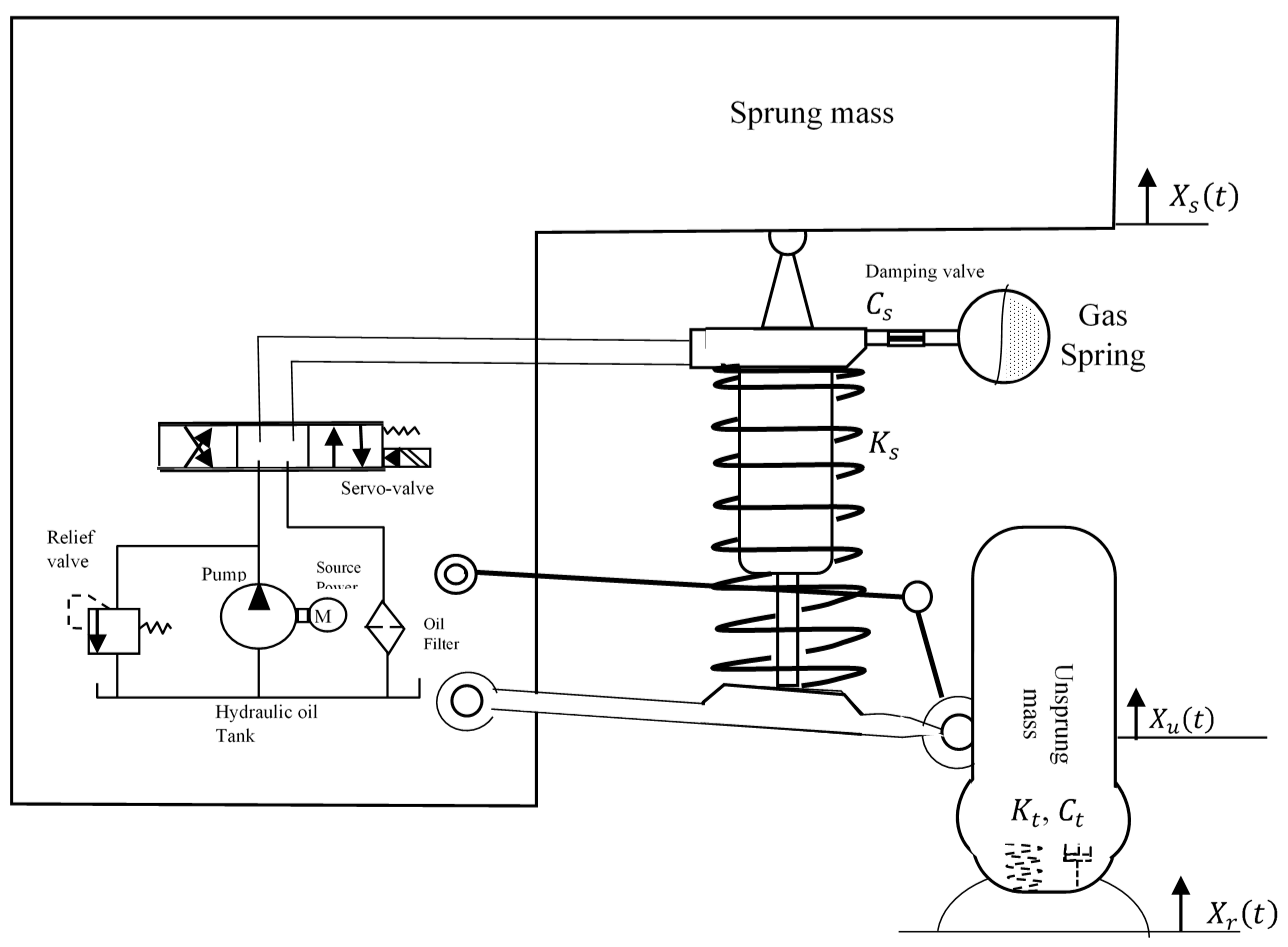
The primary purpose of the active suspension is to provide a compromise between ride comfort, car–road stability, and safety [19]. This suspension is mainly composed of a sprung mass, an unsprung mass, a spring suspension, a suspension damper, a tire, an electrohydraulic servovalve system, and other accessories [20], as shown in Figure 1. Passenger comfort definition is to isolate the sprung mass from road perturbations. Moreover, road holding definition is to handle vehicle–road stability. The electrohydraulic servovalve system (EHSS) of the active suspension generates hydraulic forces to provide a compromise between ride comfort and road holding. In

Table 1. Active suspension parameters and their descriptions.

Quantity	Description	Quantity	Description
${\mathrm{A}}_{\mathrm{p}}$	Actuator piston area, $m^2$	${\mathrm{V}}_{\mathrm{t}}$	Actuator volume, m3
${\mathrm{A}}_{\mathrm{v}}$	Spool valve projected area, m2	${\mathrm{X}}_{\mathrm{L}}$	The landing tire position, m
${\mathrm{b}}_{\mathrm{j}}$	Gaussian function width for RBFNN	${\mathrm{X}}_{\mathrm{u}}$	Unsprung mass position, m
${\mathrm{C}}_{\mathrm{d}}$	Low discharge coefficient, -	${\mathrm{X}}_{\mathrm{s}}$	Sprung mass position, m
${\mathrm{C}}_{\mathrm{tp}}$	Coefficient of leakage, m5/(Ns)	${\dot{\mathrm{X}}}_{\mathrm{s}}$	Sprung mass velocity, m/s
${\mathrm{c}}_{\mathrm{i}}$	Positive constant, -	${\ddot{\mathrm{X}}}_{\mathrm{s}}$	Sprung mass acceleration, m/s2
${\mathrm{C}}_{\mathrm{sf}}$	Parameter for static friction	${\dot{\mathrm{X}}}_{\mathrm{u}}$	Unsprung mass velocity, m/s
${\mathrm{C}}_{\mathrm{s}}$	Suspension viscous coefficient, Ns/m	${\ddot{\mathrm{X}}}_{\mathrm{u}}$	Unsprung mass acceleration, m/s2
${\mathrm{C}}_{\mathrm{t}}$	Tire viscous coefficient, Ns/m	${\mathrm{W}}_{\mathrm{i}}$	an unknown weight vector for RBFNN
${\mathrm{f}}_{\mathrm{i}}$	Unknown function i	${\check{\mathrm{X}}}_{\mathrm{u}}$	Unsprung mass position nonlinear control filter output, m
${\hat{\mathrm{f}}}_{\mathrm{i}}$	An approximate smooth function i	${\mathsf{\delta }}_0$	Positive constant, -
${\mathrm{F}}_{\mathrm{c}0}$	Coulomb friction coefficient	$\mathsf{\sigma }$	Parameter for viscous friction
${\mathrm{F}}_{\mathrm{s}0}$	Static friction coefficient	${\mathsf{\tau }}_{\mathrm{v}}$	Servovalve time constant, s
$\mathrm{g}$	Gravitational acceleration, m/$s^2$	${\mathsf{\beta }}_{\mathrm{e}}$	Effective bulk modulus, N/m2
${\mathrm{g}}_{\mathrm{i}}$	Unknown modeling function i	$\mathsf{\rho }$	Hydraulic oil density, kg/m3
${\mathrm{K}}_{\mathrm{u}\min }$	Lower bound control signal gain, m2/V	${\mathsf{\kappa }}_{\mathrm{st}}$	Positive constant, -
${\mathrm{K}}_{\mathrm{u}\max }$	Upper bound of control signal gain, m2/V	${\mathsf{\kappa }}_{\mathrm{Rh}}$	Positive constant, -
${\mathrm{K}}_{\mathrm{s}}$	Suspension spring stiffness, N/m		Adjustable factor for the road holding ratio ‘${\mathrm{R}}_{\mathrm{h}}$’, -
${\mathrm{K}}_{\mathrm{t}}$	Tire spring stiffness, N/m	${\mathsf{\phi }}_{\mathrm{i},\mathrm{j}}$	centers of the receptive field in RBFNN
$\mathrm{l}$	Number of RFBNN nodes	${\mathsf{\epsilon }}_{\mathrm{N}}$	Positive designed error of RBFNN
${\mathrm{n}}_{1,2}$,${\mathrm{m}}_{1,2,3,4}$	Positive constants	$\propto$	A virtual control function
${\mathrm{m}}_{\mathrm{u}}$	Unsprung (wheel) mass, Kg	$\zeta$	RBFNN compact set parameters
${\mathrm{m}}_{\mathrm{s}}$	Sprung (body) mass, Kg	NAC	Novel adaptive control
$\mathrm{m}$	Number of variables in the compact set	ANNC	Adaptive neural networks control system
$\mathrm{n}$	State-space order system	RBFNN	Radial basis function neural networks
${\mathrm{P}}_{\mathrm{L}}$	Operational hydraulic pressure, N/m2
${\mathrm{P}}_{\mathrm{s}}$	Pressure supply, N/m2
${\mathrm{R}}_{\mathrm{h}}$	Road holding ratio, -
$\mathrm{ST}$	Suspension travel, m
${\mathrm{ST}}_{\mathrm{D}}$	Minimum allowable of suspension travel “contraction”, m
${\mathrm{ST}}_{\mathrm{E}}$	Maximum allowable of suspension travel “expansion”, m.

, the nomenclature for the active suspension system parameters is listed with accompanying descriptions as follows.

The mathematical modeling of the quarter-car active suspension can be described as shown in Figure 1, while the sprung mass of the same is described as in [21]:

$${\mathrm{m}}_{\mathrm{s}}\left(\mathrm{t}\right){\ddot{\mathrm{X}}}_{\mathrm{s}}=-{\mathrm{F}}_{\mathrm{su}}-{\mathrm{F}}_{\mathrm{f}}+{\mathrm{A}}_{\mathrm{p}}{\mathrm{P}}_{\mathrm{L}}$$

(1)

The unsprung mass dynamic system with tire liftoff can be modeled as [22].

$${\mathrm{m}}_{\mathrm{u}}{\ddot{\mathrm{X}}}_{\mathrm{u}}=\{\begin{array}{cc}{\mathrm{F}}_{\mathrm{su}}+{\mathrm{F}}_{\mathrm{f}}-{\mathrm{A}}_{\mathrm{p}}{\mathrm{P}}_{\mathrm{L}}+{\mathrm{F}}_{\mathrm{Dt}}& \left|{\mathrm{F}}_{\mathrm{Dt}}\right|\le \left({\mathrm{m}}_{\mathrm{s}}+{\mathrm{m}}_{\mathrm{u}}\right)\mathrm{g}\\ {\mathrm{F}}_{\mathrm{su}}+{\mathrm{F}}_{\mathrm{f}}-{\mathrm{A}}_{\mathrm{p}}{\mathrm{P}}_{\mathrm{L}}\hfill & \left|{\mathrm{F}}_{\mathrm{Dt}}\right|>\left({\mathrm{m}}_{\mathrm{s}}+{\mathrm{m}}_{\mathrm{u}}\right)\mathrm{g}\end{array}$$

(2)

The spring-damper forces $F_{su}$ can be modeled as:

$$F_{su}=K_s\left(X_s-X_u\right)+C_s\left({\dot{X}}_s-{\dot{X}}_u\right)$$

(3)

The dynamic tire force $F_{Dt}$ is modeled as:

$${\mathrm{F}}_{\mathrm{Dt}}=-{\mathrm{K}}_{\mathrm{t}}\left({\mathrm{X}}_{\mathrm{u}}-{\mathrm{X}}_{\mathrm{r}}\right)-{\mathrm{C}}_{\mathrm{t}}\left({\dot{\mathrm{X}}}_{\mathrm{u}}-{\dot{\mathrm{X}}}_{\mathrm{r}}\right)$$

(4)

In this study, we considered friction forces, which consisted of a viscous friction, Coulomb friction, and a stiction friction phenomenon [23]. The friction forces are undesirable effects on the control performance. The friction forces $F_f$ of the hydraulic servosystem can be presented as in [24].

$${\mathrm{F}}_{\mathrm{f}}=\mathsf{\sigma }\left({\dot{\mathrm{X}}}_{\mathrm{s}}-{\dot{\mathrm{X}}}_{\mathrm{u}}\right)+\mathrm{sign}\left({\dot{\mathrm{X}}}_{\mathrm{s}}-{\dot{\mathrm{X}}}_{\mathrm{u}}\right)\left[{\mathrm{F}}_{\mathrm{c}0}+{\mathrm{F}}_{\mathrm{s}0}\exp \left(-\frac{\left|\left({\dot{\mathrm{X}}}_{\mathrm{s}}-{\dot{\mathrm{X}}}_{\mathrm{u}}\right)\right|}{{\mathrm{C}}_{\mathrm{sf}}}\right)\right]$$

(5)

In Equation (2), the tire must contact the road surface; otherwise, it loses the road contact (tire liftoff phenomenon). The following formula is used to express road holding:

$$\frac{\left|\mathrm{Dynamic}\mathrm{tire}\mathrm{force}\right|}{\mathrm{Suspension}\mathrm{weight}}=\frac{\left|{\mathrm{F}}_{\mathrm{Dt}}\right|}{\left({\mathrm{m}}_{\mathrm{s}}+{\mathrm{m}}_{\mathrm{u}}\right)\mathrm{g}}\le 1$$

(6)

Suspension travel limitations are other suspension restrictions. The maximum allowable suspension deflection can be represented as [17]:

$$\left|{\mathrm{X}}_{\mathrm{s}}-{\mathrm{X}}_{\mathrm{u}}\right|\le {\mathrm{ST}}_{\mathrm{D}}$$

(7)

In real operating conditions, both suspension travel limitations do not always equal the same. In this study, the suspension travel limitations became as following the form:

$${\mathrm{ST}}_{\mathrm{E}}>{\mathrm{X}}_{\mathrm{s}}-{\mathrm{X}}_{\mathrm{u}}>{\mathrm{ST}}_{\mathrm{c}}$$

(8)

where the ${\mathrm{ST}}_{\mathrm{c}}$ is a suspension travel contraction limit and the ${\mathrm{ST}}_{\mathrm{E}}$ is a suspension travel expansion limit.

The electrohydraulic servovalve system for the hydraulic actuator and the servovalve can be presented as [25]:

$$\frac{{\mathrm{V}}_{\mathrm{t}}}{2{\mathsf{\beta }}_{\mathrm{e}}}{\dot{\mathrm{P}}}_{\mathrm{L}}\left(\mathrm{t}\right)={\mathrm{C}}_{\mathrm{d}}{\mathrm{A}}_{\mathsf{\upsilon }}\left(\mathrm{t}\right)\sqrt{\frac{{\mathrm{P}}_{\mathrm{s}}-{\mathrm{P}}_{\mathrm{L}}\mathrm{sgn}({\mathrm{A}}_{\mathsf{\upsilon }}\left(\mathrm{t}\right))}{\mathsf{\rho }}}-{\mathrm{A}}_{\mathrm{p}}\left({\mathrm{X}}_{\mathrm{s}}-{\mathrm{X}}_{\mathrm{u}}\right)-{\mathrm{C}}_{\mathrm{tp}}{\mathrm{P}}_{\mathrm{L}}$$

(9)

$${\dot{\mathrm{A}}}_{\mathsf{\upsilon }}=\frac{1}{{\mathsf{\tau }}_{\mathsf{\upsilon }}}\left(-{\mathrm{A}}_{\mathsf{\upsilon }}+{\mathrm{K}}_{\mathrm{u}}\mathrm{u}\left(\mathrm{t}\right)\right)$$

(10)

In this study, a new modeling for a dynamic landing tire system was developed to avoid the dynamic tire liftoff phenomenon, as shown in Figure 2.

Dynamic tire liftoff only occurs if the unsprung mass position ${\mathrm{X}}_{\mathrm{u}}$ is higher than the road position ${\mathrm{X}}_{\mathrm{r}}$. However, Equation (6) does not consider this condition. Hence, we can rearrange Equation (6):

$${\mathrm{R}}_{\mathrm{h}}=\frac{\left({\mathrm{K}}_{\mathrm{t}}\left({\mathrm{X}}_{\mathrm{u}}-{\mathrm{X}}_{\mathrm{r}}\right)+{\mathrm{C}}_{\mathrm{t}}\left({\dot{\mathrm{X}}}_{\mathrm{u}}-{\dot{\mathrm{X}}}_{\mathrm{r}}\right)\right)}{\left({\mathrm{m}}_{\mathrm{s}}+{\mathrm{m}}_{\mathrm{u}}\right)\mathrm{g}}\le 1$$

(11)

where ${\mathrm{R}}_{\mathrm{h}}$ is a road holding ratio.

Therefore, the vertical tire displacement $\left({\mathrm{X}}_{\mathrm{u}}-{\mathrm{X}}_{\mathrm{r}}\right)$ can use ${\mathrm{X}}_{\mathrm{L}}$ as a required tire landing position.

$${\mathrm{K}}_{\mathrm{t}}{\mathrm{X}}_{\mathrm{L}}+{\mathrm{C}}_{\mathrm{t}}{\dot{\mathrm{X}}}_{\mathrm{L}}\le \left({\mathrm{m}}_{\mathrm{s}}+{\mathrm{m}}_{\mathrm{u}}\right)$$

(12)

In order to avoid tire liftoff, the tire landing position must be evaluated before the critical road holding ratio ‘${\mathrm{R}}_{\mathrm{h}}=1$’. Thus, the dynamic landing position ${\mathrm{X}}_{\mathrm{L}}$ is created in the following form:

$${\dot{\mathrm{X}}}_{\mathrm{L}}\left(\mathrm{t}\right)=\{\begin{array}{cc}0& {\mathrm{R}}_{\mathrm{h}}\left(\mathrm{t}\right)<1\\ \frac{{\mathrm{K}}_{\mathrm{t}}}{{\mathrm{C}}_{\mathrm{t}}}\left({\mathrm{X}}_{\mathrm{L}}\left(\mathrm{t}\right)+\frac{{\mathsf{\kappa }}_{\mathrm{w}}\left({\mathrm{m}}_{\mathrm{s}}+{\mathrm{m}}_{\mathrm{u}}\right)\mathrm{g}}{{\mathrm{K}}_{\mathrm{t}}}\left({\mathrm{R}}_{\mathrm{h}}\left(\mathrm{t}\right)-1\right)\right)& {\mathsf{\kappa }}_{\mathrm{w}}^{-1}\ge {\mathrm{R}}_{\mathrm{h}}\left(\mathrm{t}\right)\ge 1\end{array}$$

(13)

where the ${\mathsf{\kappa }}_{\mathrm{w}}$ is an adjustable factor for the road holding ratio $\left(0\le {\mathsf{\kappa }}_{\mathrm{w}}\le 1\right)$.

Moreover, the differential road holding ${\dot{\mathrm{R}}}_{\mathrm{h}}$ is differentially determined, as follows:

Equations (12) and (13) can represent the dynamic landing tire system into the state-space modeling system.

$${\dot{\mathrm{R}}}_{\mathrm{h}}\left(\mathrm{t}\right)=\begin{array}{cc}\frac{{\mathrm{K}}_{\mathrm{t}}\left({\dot{\mathrm{X}}}_{\mathrm{u}}-{\dot{\mathrm{X}}}_{\mathrm{r}}\right)+{\mathrm{C}}_{\mathrm{t}}\left({\ddot{\mathrm{X}}}_{\mathrm{u}}-{\ddot{\mathrm{X}}}_{\mathrm{r}}\right)}{{\mathsf{\kappa }}_{\mathrm{w}}\left({\mathrm{m}}_{\mathrm{s}}+{\mathrm{m}}_{\mathrm{u}}\right)\mathrm{g}}& {\mathrm{R}}_{\mathrm{h}}\left(\mathrm{t}\right)\end{array}\le {\mathsf{\kappa }}_{\mathrm{w}}^{-1}$$

(14)

3. Control Design

This section consists of three subsections: Nonlinear control filter system, adaptive neural networks’ backstepping control system, and zero dynamic systems.

3.1. Nonlinear Control Filter

In [11], a nonlinear control filter was developed to adjust the trade-off between passenger comfort and suspension travel for a quarter-car active suspension system. In this study, we redesigned the nonlinear control filter by modifying a nonlinear tire land function $\mathsf{\varphi }\left({\mathrm{X}}_{\mathrm{L}}\right)$. The input filter was the unsprung mass position ${\mathrm{X}}_{\mathrm{u}}$. Therefore, the nonlinear control filter was able to compromise between passenger comfort and road holding and also suspension travel, as follows:

$${\dot{\check{\mathrm{X}}}}_{\mathrm{u}}=-\left({\mathsf{\delta }}_0+{\mathsf{\kappa }}_{\mathrm{st}}\mathsf{\psi }\left(\mathrm{ST}\right)+{\mathsf{\kappa }}_{\mathrm{Rh}}\mathsf{\varphi }\left({\mathrm{X}}_{\mathrm{L}}\right)\right)\left({\breve{\mathrm{X}}}_{\mathrm{u}}-{\mathrm{X}}_{\mathrm{u}}\right)$$

(15)

where the symbols ${\mathsf{\delta }}_0$, ${\mathsf{\kappa }}_{\mathrm{st}}$, and ${\mathsf{\kappa }}_{\mathrm{Rh}}$ are positive constants, and the suspension travel $\mathrm{ST},$ $\mathrm{ST}={\mathrm{X}}_{\mathrm{s}}-{\mathrm{X}}_{\mathrm{u}}$.

The nonlinear function of suspension travel $\mathsf{\psi }\left(\mathrm{ST}\right)$ is a positive nonlinear function.

$$\mathsf{\psi }\left(\mathrm{ST}\right)=\{\begin{array}{cc}{\left(\frac{\mathrm{ST}-{\mathrm{m}}_2}{{\mathrm{m}}_1}\right)}^4,& \mathrm{ST}<{\mathrm{m}}_2\\ 0,& {\mathrm{m}}_3\ge \mathrm{ST}\ge {\mathrm{m}}_2\\ {\left(\frac{\mathrm{ST}-{\mathrm{m}}_3}{{\mathrm{m}}_4}\right)}^4,& \mathrm{ST}>{\mathrm{m}}_3\end{array}$$

(16)

where ${\mathrm{m}}_2$ is a chosen constant $0\ge {\mathrm{m}}_2\ge {\mathrm{ST}}_{\mathrm{c}}$, ${\mathrm{m}}_3$ is a chosen constant ${\mathrm{ST}}_{\mathrm{E}}\ge {\mathrm{m}}_3\ge 0$, and the ${\mathrm{m}}_1{\mathrm{and}\mathrm{m}}_4$ are positive constants.

The landing tire nonlinear function $\mathsf{\varphi }\left({\mathrm{X}}_{\mathrm{L}}\right)$ is a positive nonlinear function and evaluates as follows.

$$\mathsf{\varphi }\left({\mathrm{X}}_{\mathrm{L}}\right)=\{\begin{array}{cc}{\left(\frac{{\mathrm{X}}_{\mathrm{L}}+{\mathrm{n}}_2}{{\mathrm{n}}_1}\right)}^4& {\mathsf{\kappa }}_{\mathrm{w}}^{-1}\ge {\mathrm{R}}_{\mathrm{h}}\ge 1\\ 0& {\mathrm{R}}_{\mathrm{h}}<1\end{array}$$

(17)

where ${\mathrm{n}}_1$ and ${\mathrm{n}}_1$ are positive constants.

It can be concluded that the flow chart of the nonlinear control filter dynamic system is sketched in Figure 3. When the filter dead-zone $\left({\mathrm{R}}_{\mathrm{h}}<1,{\mathrm{m}}_3\ge \mathrm{ST}\ge {\mathrm{m}}_2\right)$ was activated, the nonlinear bandwidth filter became a chosen small constant ${\mathsf{\delta }}_0$ to obtain passenger comfort. Otherwise, at least one of the suspension constraints $\left({\mathrm{m}}_3<\mathrm{ST},\mathrm{ST}<{\mathrm{m}}_2,{\mathsf{\kappa }}_{\mathrm{w}}^{-1}\ge {\mathrm{R}}_{\mathrm{h}}\ge 1\right)$ was expected; the nonlinear function $\left(\mathsf{\psi }\left(\mathrm{ST}\right),\mathsf{\varphi }\left({\mathrm{X}}_{\mathrm{L}}\right)\right)$ rapidly increased the filter bandwidth. Thus, the suspension travel became stiff:

The state-space modeling system was built from Equations (1), (2), (9), (10), and (13)–(15). Therefore, the state-space modeling of the filtered active suspension system had nine variables, as follows.

State-space modeling system:

$${\mathrm{X}}_1={\mathrm{X}}_{\mathrm{s}},{\mathrm{X}}_2={\dot{\mathrm{X}}}_{\mathrm{s}},{\mathrm{X}}_3={\mathrm{C}}_{\mathrm{h}}{\mathrm{P}}_{\mathrm{L}},{\mathrm{X}}_4={\mathrm{C}}_{\mathrm{v}}{\mathrm{A}}_{\mathrm{v}},{\mathrm{X}}_5={\check{\mathrm{X}}}_{\mathrm{u}},{\mathrm{X}}_6={\mathrm{X}}_{\mathrm{u}},{\mathrm{X}}_7={\dot{\mathrm{X}}}_{\mathrm{u}},{\mathrm{X}}_8={\mathrm{X}}_{\mathrm{L}},{\mathrm{X}}_9={\mathrm{R}}_{\mathrm{h}}$$

$${\dot{\mathrm{X}}}_1={\mathrm{X}}_2$$

$$\begin{gathered} {\dot{\mathrm{X}}}_2=-\frac{{\mathrm{K}}_{\mathrm{s}}}{{\mathrm{m}}_{\mathrm{s}}}\left({\mathrm{X}}_1-{\mathrm{X}}_3\right)-\frac{{\mathrm{C}}_{\mathrm{s}}}{{\mathrm{m}}_{\mathrm{s}}}\left({\mathrm{X}}_2-{\mathrm{X}}_4\right)+\frac{{\mathrm{A}}_{\mathrm{p}}}{{\mathrm{m}}_{\mathrm{s}}}{\mathrm{X}}_5 \\ {\dot{\mathrm{X}}}_3=\frac{2{\mathsf{\beta }}_e{\mathrm{C}}_{\mathrm{d}}}{{\mathrm{V}}_{\mathrm{t}}}{\mathrm{X}}_4\sqrt{\frac{{\mathrm{P}}_{\mathrm{s}}-{\mathrm{X}}_3\mathrm{sgn}\left({\mathrm{X}}_4\right)}{\mathsf{\rho }}}-\frac{2{\mathsf{\beta }}_e{\mathrm{A}}_{\mathrm{p}}}{{\mathrm{V}}_{\mathrm{t}}}\left({\mathrm{X}}_2-{\mathrm{X}}_7\right)+\frac{2{\mathsf{\beta }}_e{\mathrm{C}}_{\mathrm{tp}}}{{\mathrm{V}}_{\mathrm{t}}}{\mathrm{X}}_3 \end{gathered}$$

$${\dot{\mathrm{X}}}_4=\frac{1}{{\mathsf{\tau }}_{\mathrm{v}}}\left(-{\mathrm{X}}_4+{\mathrm{K}}_{\mathrm{u}}\mathrm{u}\left(\mathrm{t}\right)\right)$$

(18)

$${\dot{\mathrm{X}}}_5=-\left({\mathsf{\delta }}_0+{\mathsf{\kappa }}_{\mathrm{st}}\mathsf{\psi }\left(\mathsf{\eta }\right)+{\mathsf{\kappa }}_{\mathrm{Rh}}\mathsf{\varphi }\left({\mathrm{X}}_8\right)\right)\left({\mathrm{X}}_5-{\mathrm{X}}_6\right)$$

$${\dot{\mathrm{X}}}_6={\mathrm{X}}_7$$

$${\dot{\mathrm{X}}}_7=\{\begin{array}{cc}{\mathrm{K}}_{\mathrm{s}}\left({\mathrm{X}}_1-{\mathrm{X}}_6\right)+{\mathrm{C}}_{\mathrm{s}}\left({\mathrm{X}}_2-{\mathrm{X}}_7\right)-{\mathrm{A}}_{\mathrm{p}}{\mathrm{X}}_3-{\mathrm{K}}_{\mathrm{t}}\left({\mathrm{X}}_6-{\mathrm{X}}_{\mathrm{r}}\right)-{\mathrm{C}}_{\mathrm{t}}\left({\mathrm{X}}_7-\dot{{\mathrm{X}}_{\mathrm{r}}}\right)& {\mathrm{X}}_9\le {\mathsf{\kappa }}_{\mathrm{w}}^{-1}\\ {\mathrm{K}}_{\mathrm{s}}\left({\mathrm{X}}_1-{\mathrm{X}}_6\right)+{\mathrm{C}}_{\mathrm{s}}\left({\mathrm{X}}_2-{\mathrm{X}}_7\right)-{\mathrm{A}}_{\mathrm{p}}{\mathrm{X}}_3& {\mathrm{X}}_9>{\mathsf{\kappa }}_{\mathrm{w}}^{-1}\end{array}$$

$${\dot{\mathrm{X}}}_8=\{\begin{array}{cc}0& {\mathrm{X}}_9<1\\ -\frac{{\mathrm{K}}_{\mathrm{t}}}{{\mathrm{C}}_{\mathrm{t}}}\left({\mathrm{X}}_8-\frac{{\mathsf{\kappa }}_{\mathrm{w}}\left({\mathrm{m}}_{\mathrm{s}}+{\mathrm{m}}_{\mathrm{u}}\right)\mathrm{g}}{{\mathrm{K}}_{\mathrm{t}}}\left({\mathrm{X}}_9-1\right)\right)& {\mathsf{\kappa }}_{\mathrm{w}}^{-1}\ge {\mathrm{X}}_9\ge 1\end{array}$$

$$\begin{gathered} {\dot{\mathrm{X}}}_9=\frac{1}{{\mathsf{\kappa }}_{\mathrm{w}}\left({\mathrm{m}}_{\mathrm{s}}+{\mathrm{m}}_{\mathrm{u}}\right)\mathrm{g}}\left\{-{\mathrm{K}}_{\mathrm{t}}\left({\mathrm{X}}_7-\dot{\mathrm{r}}\right)-{\mathrm{K}}_{\mathrm{s}}{\mathrm{C}}_{\mathrm{t}}\left({\mathrm{X}}_1-{\mathrm{X}}_6\right)-{\mathrm{C}}_{\mathrm{s}}{\mathrm{C}}_{\mathrm{t}}\left({\mathrm{X}}_2-{\mathrm{X}}_7\right)+{\mathrm{C}}_{\mathrm{t}}{\mathrm{A}}_{\mathrm{p}}{\mathrm{X}}_3 \\ +{\mathrm{C}}_{\mathrm{t}}{\mathrm{K}}_{\mathrm{t}}\left({\mathrm{X}}_6-{\mathrm{X}}_{\mathrm{r}}\right)+{\mathrm{C}}_{\mathrm{t}}^2\left({\mathrm{X}}_7-\dot{{\mathrm{X}}_{\mathrm{r}}}\right)+{\mathrm{C}}_{\mathrm{t}}\ddot{\mathrm{r}}\right\},{\mathrm{X}}_9\le {\mathsf{\kappa }}_{\mathrm{w}}^{-1} \end{gathered}$$

$$\mathrm{y}={\mathrm{X}}_1-{\mathrm{X}}_5$$

3.2. Adaptive Neural Networks’ Backstepping Control Design

In this section, an adaptive neural networks’ backstepping was developed for the recursive closed-loop system in Equation (18). Lyapunov’s stability theory was employed to guarantee control stability. One advantages of this technique is that it allows circumventing the unmodeled model uncertainties of multiple dynamic systems. Several research studies have applied the backstepping control technique to overcome the inherent nonlinearities and uncertainties of the system. The backstepping design complicity is to determine regression matrices of uncertain nonlinear functions. In order to linearize the state-space modeling and simplify the backstepping control system, a linear radial basis function neural networks (RBFNN) was implemented, and could deal with unknown functions. Hence, the state space modeling of the adaptive neural networks’ control (ANNC) design was reduced to fourth orders.

$$\begin{gathered} {\dot{\mathrm{X}}}_1={\mathrm{X}}_2 \\ {\dot{\mathrm{X}}}_2={\mathrm{X}}_3+{\mathrm{g}}_2\left(\mathrm{X}\right) \\ {\dot{\mathrm{X}}}_3={\mathrm{X}}_4+{\mathrm{g}}_3\left(\mathrm{X}\right) \\ {\dot{\mathrm{X}}}_4=\mathsf{\beta }\mathrm{u}\left(\mathrm{t}\right)+{\mathrm{g}}_4\left(\mathrm{X}\right) \\ \mathrm{y}={\mathrm{X}}_1-{\mathrm{X}}_5\forall \left[{\mathrm{X}}_1,{\mathrm{X}}_2,{\mathrm{X}}_3,{\mathrm{X}}_4\right]\in {\mathsf{\Omega }}_{\mathrm{X}}\subset {\mathrm{R}}^4 \end{gathered}$$

(19)

Thus, the functions ${\mathrm{g}}_2\left(\mathrm{X}\right),{\mathrm{g}}_3\left(\mathrm{X}\right),{\mathrm{g}}_4\left(\mathrm{X}\right)$ and the parameter $\mathsf{\beta }$ are chosen as follows.

$$\begin{gathered} {\mathrm{g}}_2\left(\mathrm{X}\right)=-{\mathrm{X}}_3-\frac{{\mathrm{K}}_{\mathrm{s}}}{{\mathrm{m}}_{\mathrm{s}}}\left({\mathrm{X}}_1-{\mathrm{X}}_6\right)-\frac{{\mathrm{C}}_{\mathrm{s}}}{{\mathrm{m}}_{\mathrm{s}}}\left({\mathrm{X}}_2-{\mathrm{X}}_7\right)+\frac{{\mathrm{A}}_{\mathrm{p}}}{{\mathrm{m}}_{\mathrm{s}}}{\mathrm{X}}_3 \\ {\mathrm{g}}_3\left(\mathrm{X}\right)=-{\mathrm{X}}_4+\frac{2{\mathsf{\beta }}_e{\mathrm{C}}_{\mathrm{d}}}{{\mathrm{V}}_{\mathrm{t}}}{\mathrm{X}}_4\sqrt{\frac{{\mathrm{P}}_{\mathrm{s}}-{\mathrm{X}}_3\mathrm{sgn}\left({\mathrm{X}}_4\right)}{\mathsf{\rho }}}-\frac{2{\mathsf{\beta }}_e{\mathrm{A}}_{\mathrm{p}}}{{\mathrm{V}}_{\mathrm{t}}}\left({\mathrm{X}}_2-{\mathrm{X}}_7\right)+\frac{2{\mathsf{\beta }}_e{\mathrm{C}}_{\mathrm{tp}}}{{\mathrm{V}}_{\mathrm{t}}}{\mathrm{X}}_3 \\ {\mathrm{g}}_4\left(\mathrm{X}\right)=-\frac{{\mathrm{X}}_4}{{\mathsf{\tau }}_{\mathrm{v}}} \\ \mathsf{\beta }=\frac{{\mathrm{K}}_{\mathrm{u}}}{{\mathsf{\tau }}_{\mathrm{v}}} \end{gathered}$$

(20)

In order to approximate the unknown functions ${\mathrm{g}}_{\mathrm{i}}\left(\mathsf{\zeta }\right)$, we needed to know the aspect of the radial basis function neural network. The radial basis function neural networks (RBFNN) can approximate nonlinear and unknown bounding functions. In this study, we used a linear RBFNN to approximate the unknown functions of the modeling system. The linear RBFNN had one hidden layer, a fixed size, and fixed moving basis functions [26,27]. Therefore, the unknown smooth functions ${\mathrm{f}}_{\mathrm{i}}\left(\mathsf{\zeta }\right)$ could be presented as [28,29]:

$${\mathrm{f}}_{\mathrm{i}}\left(\mathsf{\zeta }\right)={\mathrm{W}}_{\mathrm{i}}^{\mathrm{T}}{\mathrm{H}}_{\mathrm{i}}\left(\mathsf{\zeta }\right)+{\mathsf{\epsilon }}_{\mathrm{i}},\mathrm{i}=1,2,\dots ,\mathrm{n},\forall \mathsf{\zeta }\in {\mathsf{\Omega }}_{\mathsf{\zeta }}\subset {ℝ}^{\mathrm{m}}$$

(21)

where the input vector $\mathsf{\zeta }\in {\mathsf{\Omega }}_{\mathsf{\zeta }}\subset {ℝ}^{\mathrm{m}}$, the ${\mathsf{\epsilon }}_{\mathrm{i}}$ is the approximation error, the ${\mathrm{W}}_{\mathrm{i}}^{\mathrm{T}}$ is an unknown weight vector, ${\mathrm{W}}_{\mathrm{i}}^{\mathrm{T}}={\left[\begin{array}{ccc}{\mathrm{W}}_1& {\mathrm{W}}_2& \begin{array}{cc}\dots & {\mathrm{W}}_{\mathrm{l}}\end{array}\end{array}\right]}_{\mathrm{i}}^{\mathrm{T}}$, the ${\mathrm{H}}_{\mathrm{i}}\left(\mathsf{\zeta }\right)$ is a basis function vector, ${\mathrm{H}}_{\mathrm{i}}\left(\mathsf{\zeta }\right)={\left[\begin{array}{ccc}{\mathrm{h}}_1\left(\mathsf{\zeta }\right)& {\mathrm{h}}_2\left(\mathsf{\zeta }\right)& \begin{array}{cc}\dots & {\mathrm{h}}_{\mathrm{l}}\left(\mathsf{\zeta }\right)\end{array}\end{array}\right]}_{\mathrm{i}}$, and the ${\mathrm{h}}_{\mathrm{i}}\left(\mathsf{\zeta }\right),\mathrm{i}=1,\dots ,\mathrm{l}$ are hidden Gaussian functions, which satisfy:

$${\mathrm{h}}_{\mathrm{i}}\left(\mathsf{\zeta }\right)={\mathrm{e}}^{-\left\{\frac{\zeta -{\mathsf{\phi }}_{i,j}{}^2}{2{\mathrm{b}}_{\mathrm{j}}^2}\right\}},\mathrm{i}=1,\dots ,\mathrm{l},\zeta =\left[{\mathsf{\zeta }}_1,{\mathsf{\zeta }}_2,\dots ,{\mathsf{\zeta }}_{\mathrm{m}}\right]\forall \mathsf{\zeta }\in {\mathsf{\Omega }}_{\mathsf{\zeta }}\subset {ℝ}^{\mathrm{l}}$$

(22)

where the $\left\{{\mathsf{\phi }}_{i,j},{\mathrm{b}}_{\mathrm{j}},\mathrm{i}=1,\dots ,\mathrm{l}\mathrm{and}\mathrm{j}=1,\dots ,\mathrm{m}\right\}$ are the centers of the receptive field and the width of Gaussian function, respectively.

Therefore, approximate smooth functions ${\widehat{f}}_i\left(\mathsf{\zeta }\right)$ could be estimated by RBFNN as follows:

$${\hat{\mathrm{f}}}_{\mathrm{i}}\left(\mathsf{\zeta }\right)={\hat{\mathrm{W}}}_{\mathrm{i}}^{\mathrm{T}}{\mathrm{H}}_{\mathrm{i}}\left(\mathsf{\zeta }\right),\mathrm{i}=1,2,\dots ,\mathrm{n}\forall \mathsf{\zeta }\in {\mathsf{\Omega }}_{\mathsf{\zeta }}\subset {ℝ}^{\mathrm{m}}$$

(23)

To minimize the approximation error, the optimal weight value ‘${\mathrm{W}}_i$’ of the RBFNN was defined [30]:

$${\mathrm{W}}_{\mathrm{i}}:=\arg \underset{{\hat{\mathrm{W}}}_{\mathrm{i}}\in {\mathrm{R}}^{\mathrm{n}}}{\min }\left\{\underset{\mathsf{\zeta }\in {\mathsf{\Omega }}_{\mathrm{i}}}{\sup }\left|\right|{\mathrm{f}}_{\mathrm{i}}\left(\mathsf{\zeta }\right)-{\hat{\mathrm{f}}}_{\mathrm{i}}\left(\mathsf{\zeta }\right)\right|\left|\right\},{\mathrm{W}}_{\mathrm{i}}\mathrm{is}\mathrm{l}\times \mathrm{m},\forall \mathsf{\zeta }\in {\mathsf{\Omega }}_{\mathrm{i}}$$

(24)

As a result, a tiny positive design error ${\mathsf{\epsilon }}_{\mathrm{N}}$ could have occurred:

$$\max \left|\right|f\left(\mathsf{\zeta }\right)-\widehat{f}\left(\mathsf{\zeta }\right)\left|\right|\le {\mathsf{\epsilon }}_{\mathrm{N}}$$

(25)

where $f\left(\mathsf{\zeta }\right)=\left[\begin{array}{ccc}{\mathrm{f}}_1\left(\mathsf{\zeta }\right)& {\mathrm{f}}_2\left(\mathsf{\zeta }\right)& \begin{array}{cc}\dots & {\mathrm{f}}_{\mathrm{n}}\left(\mathsf{\zeta }\right)\end{array}\end{array}\right]$ and $\widehat{f}\left(\mathsf{\zeta }\right)=\left[\begin{array}{ccc}{\hat{\mathrm{f}}}_1\left(\mathsf{\zeta }\right)& {\hat{\mathrm{f}}}_2\left(\mathsf{\zeta }\right)& \begin{array}{cc}\dots & {\hat{\mathrm{f}}}_{\mathrm{n}}\left(\mathsf{\zeta }\right)\end{array}\end{array}\right]$.

The “centers and widths” of the RBFNN were chosen based on a range of input values. Therefore, we applied a gradient descent learning algorithm to obtain the optimal RBFNN parameters such as the centers ${\mathsf{\phi }}_{i,j}$, widths ${\mathrm{b}}_{\mathrm{j}}$, and number of nodes $\mathrm{l}$.

The backstepping control was organized into four backstepping control steps, as follows.

Step 1: Sprung mass velocity

The control coordinate ${\mathrm{Z}}_1$ was defined as:

$${\mathrm{Z}}_1={\mathrm{X}}_1-{\mathrm{X}}_5$$

(26)

To stabilize the controller, let us consider a quadratic Lyapunov function candidate ${\mathrm{V}}_1:$

$${\mathrm{V}}_1=\frac{1}{2}{\mathrm{z}}_1^2\left(27\right)$$

(27)

The Lyapunov derivative function ${\dot{\mathrm{V}}}_1$ of step 1 becomes:

$${\dot{\mathrm{V}}}_1={\mathrm{Z}}_1{\dot{\mathrm{Z}}}_1={\mathrm{Z}}_1\left({\dot{\mathrm{X}}}_1-{\dot{\mathrm{X}}}_5\right)$$

(28)

To stabilize the system, the derivative control coordinate ${\dot{\mathrm{Z}}}_1$ becomes:

$${\dot{\mathrm{Z}}}_1={\mathrm{Z}}_2+{\propto }_1-{\dot{\mathrm{X}}}_5=-{\mathrm{c}}_1{\mathrm{Z}}_1$$

(29)

where ${\mathrm{c}}_1$ is a positive constant.

Then, the virtual control function ${\propto }_1$ is:

$${\propto }_1={\dot{\mathrm{X}}}_5-{\mathrm{c}}_1{\mathrm{Z}}_1$$

(30)

Substitute ${\propto }_1$ into ${\dot{\mathrm{V}}}_1$:

$${\dot{\mathrm{V}}}_1={\mathrm{Z}}_1{\mathrm{Z}}_2-{\mathrm{c}}_1{\mathrm{Z}}_1^2\left(31\right)$$

(31)

Step 2: Sprung mass dynamic acceleration

We can define the virtual control coordinate ${\mathrm{Z}}_{\mathrm{i}}$ as:

$${\dot{\mathrm{Z}}}_{\mathrm{i}}={\dot{\mathrm{X}}}_{\mathrm{i}}-{\dot{\propto }}_{\mathrm{i}-1}$$

(32)

Lemma 1: 

The control derivative function${\dot{\propto }}_{i-1}$produces two parts, namely, a countable part${\dot{\propto }}_{{\left(i-1\right)}_c}$and an uncountable part${\dot{\propto }}_{{\left(i-1\right)}_u}$ [31]. The ${\propto }_{i-1}$ is defined.

$${\propto }_{\mathrm{i}-1}\equiv {\propto }_{\mathrm{i}-1}\left({\mathrm{X}}_1,\dots ,{\mathrm{X}}_{\mathrm{i}},{\hat{\mathrm{W}}}_{\mathrm{i}-1}\right)$$

Then, the partial derivative of the function ${\propto }_{i-1}$ is:

$${\dot{\propto }}_{\mathrm{i}-1}=\frac{\partial {\propto }_{\mathrm{i}-1}}{\partial {\mathrm{X}}_1}{\mathrm{X}}_2+\dots +\frac{\partial {\propto }_{\mathrm{i}-1}}{\partial {\mathrm{X}}_{\mathrm{i}-1}}{\mathrm{X}}_{\mathrm{i}}+\frac{\partial {\propto }_{\mathrm{i}-1}}{\partial {\hat{\mathrm{W}}}_{\mathrm{i}-1}}{\dot{\hat{\mathrm{W}}}}_{\mathrm{i}-1}$$

Therefore, the uncountable part ${\dot{\propto }}_{{\left(i-1\right)}_u}$ consists of unknown smooth functions:

$${\dot{\propto }}_{{\left(\mathrm{i}-1\right)}_{\mathrm{u}}}={\displaystyle \sum }_{\mathrm{k}=1}^{\mathrm{i}-1}\frac{\partial {\propto }_{\mathrm{i}-1}}{\partial {\mathrm{X}}_{\mathrm{k}}}{\mathrm{g}}_{\mathrm{k}}\left(\mathrm{X}\right)+\frac{\partial {\propto }_{\mathrm{i}-1}}{\partial {\hat{\mathrm{W}}}_{\mathrm{i}-1}}{\dot{\hat{\mathrm{W}}}}_{\mathrm{i}-1}$$

The countable part ${\dot{\propto }}_{{\left(i-1\right)}_c}$ is a smooth function described as:

$${\dot{\propto }}_{{\left(\mathrm{i}-1\right)}_{\mathrm{c}}}={\displaystyle \sum }_{\mathrm{k}=1}^{\mathrm{i}-1}\frac{\partial {\propto }_{\mathrm{i}-1}}{\partial {\mathrm{X}}_{\mathrm{k}}}{\mathrm{X}}_{\mathrm{k}+1}$$

Thus, the total unknown functions at step i-1 are defined:

$${\dot{\propto }}_{{\left(\mathrm{i}-1\right)}_{\mathrm{c}}}={\displaystyle \sum }_{\mathrm{k}=1}^{\mathrm{i}-1}\frac{\partial {\propto }_{\mathrm{i}-1}}{\partial {\mathrm{X}}_{\mathrm{k}}}{\mathrm{X}}_{\mathrm{k}+1}$$

The unknown function $f_i\left(X\right)$ can be represented by the RBFNN as follows:

$${\mathrm{f}}_{\mathrm{i}}\left(\mathrm{X}\right)={\mathrm{W}}_{\mathrm{i}}^{\mathrm{T}}{\mathrm{h}}_{\mathrm{i}}\left(\mathsf{\zeta }\right)+{\mathsf{\epsilon }}_{\mathrm{i}},\mathsf{\zeta }\equiv \mathrm{X},\forall \mathsf{\zeta }\in {\mathsf{\Omega }}_{\mathsf{\zeta }}\subset {ℝ}^{\mathrm{m}}$$

Therefore, the Lyapunov function candidate $V_2$ design is selected:

$${\mathrm{V}}_2={\mathrm{V}}_1+\frac{1}{2}{\mathrm{Z}}_2^2+\frac{1}{2}{\tilde{\mathrm{W}}}_2{\mathsf{\Gamma }}_2^{-1}{\tilde{\mathrm{W}}}_2$$

(33)

By applying Lemma 1, the Lyapunov derivative function candidate ${\dot{V}}_2$ becomes:

$${\dot{\mathrm{V}}}_2={\dot{\mathrm{V}}}_1+{\mathrm{Z}}_2\left({\mathrm{X}}_3+{\mathrm{W}}_2^{\mathrm{T}}{\mathrm{h}}_2\left(\mathsf{\zeta }\right)+{\mathsf{\epsilon }}_2-{\dot{\propto }}_{1_{\mathrm{c}}}\right)+{\tilde{\mathrm{W}}}_2{\mathsf{\Gamma }}_2{}^{-1}{\dot{\hat{\mathrm{W}}}}_2$$

(34)

The adaptive RBFNN law ${\dot{\widehat{W}}}_2$ is defined [32,33]:

$${\dot{\hat{\mathrm{W}}}}_2={\mathsf{\Gamma }}_2{\mathrm{Z}}_2{\mathrm{h}}_2\left(\mathsf{\zeta }\right)-{\mathsf{\Gamma }}_2{\mathsf{\sigma }}_{\mathsf{\theta }}{}_2{\hat{\mathrm{W}}}_2$$

(35)

where the ${\Gamma }_2$ is a positive definite matrix and the ${\sigma }_{\theta }{}_2$ is a positive constant.

Therefore, the selected virtual control${\propto }_2$is:

$${\propto }_2=-{\mathrm{Z}}_1-{\mathrm{c}}_2{\mathrm{Z}}_2-{\hat{\mathrm{W}}}_2^{\mathrm{T}}{\mathrm{h}}_2\left(\mathsf{\zeta }\right)+{\dot{\propto }}_{1_{\mathrm{c}}}$$

(36)

By substituting Equations (35) and (36) into the Lyapunov derivative function${\dot{V}}_2$:

$${\dot{\mathrm{V}}}_2=-{\mathrm{c}}_1{\mathrm{Z}}_1^2-{\mathrm{c}}_2{\mathrm{Z}}_2^2+{\mathrm{Z}}_3{\mathrm{Z}}_2+{\mathrm{Z}}_2{\mathsf{\epsilon }}_2-{\mathsf{\sigma }}_{\mathsf{\theta }}{}_2{\tilde{\mathrm{W}}}_2{\hat{\mathrm{W}}}_2$$

(37)

The function${\dot{V}}_2$is moved to the next step.

Step 3: Hydraulic actuator dynamic system

The virtual control coordinate ${\mathrm{Z}}_3$ is:

$${\mathrm{Z}}_3={\mathrm{X}}_3-{\propto }_2$$

(38)

Hence, the ${\mathrm{Z}}_3$ derivative function becomes

$${\dot{\mathrm{Z}}}_3={\dot{\mathrm{X}}}_3-{\dot{\propto }}_2={\mathrm{X}}_4+{\mathrm{g}}_3\left(\mathrm{X}\right)-{\dot{\propto }}_2$$

(39)

The Lyapunov function candidate ${\mathrm{V}}_{\mathrm{i}}$ design is selected:

$${\mathrm{V}}_3={\mathrm{V}}_2+\frac{1}{2}{\mathrm{Z}}_3^2+\frac{1}{2}{\tilde{\mathrm{W}}}_3{\mathsf{\Gamma }}_3^{-1}{\tilde{\mathrm{W}}}_3$$

(40)

By applying Lemma 1, the Lyapunov derivative function candidate ${\dot{\mathrm{V}}}_3$ becomes:

$${\dot{\mathrm{V}}}_3={\dot{\mathrm{V}}}_2+{\mathrm{Z}}_3\left({\mathrm{X}}_4+{\mathrm{W}}_3^{\mathrm{T}}{\mathrm{h}}_3\left(\mathsf{\zeta }\right)+{\mathsf{\epsilon }}_3-{\dot{\propto }}_{2_{\mathrm{c}}}\right)+{\tilde{\mathrm{W}}}_3{\mathsf{\Gamma }}_3{}^{-1}{\dot{\hat{\mathrm{W}}}}_3$$

(41)

Therefore, the selected virtual control ${\propto }_3$ is:

$${\propto }_3=-{\mathrm{Z}}_2-{\mathrm{c}}_3{\mathrm{Z}}_3-{\hat{\mathrm{W}}}_3^{\mathrm{T}}{\mathrm{h}}_3\left(\mathsf{\zeta }\right)+{\dot{\propto }}_{2_{\mathrm{c}}}$$

(42)

By substituting Equation (42) into the Lyapunov derivative function ${\dot{\mathrm{V}}}_2$:

$${\dot{\mathrm{V}}}_3=-{\mathrm{c}}_1{\mathrm{Z}}_1^2-{\mathrm{c}}_2{\mathrm{Z}}_2^2-{\mathrm{c}}_3{\mathrm{Z}}_3^2+{\mathrm{Z}}_4{\mathrm{Z}}_3+{\mathrm{Z}}_2{\mathsf{\epsilon }}_2+{\mathrm{Z}}_3{\mathsf{\epsilon }}_3-{\mathsf{\sigma }}_{\mathsf{\theta }}{}_2{\tilde{\mathrm{W}}}_2{\hat{\mathrm{W}}}_2-{\mathsf{\sigma }}_{\mathsf{\theta }}{}_3{\tilde{\mathrm{W}}}_3{\hat{\mathrm{W}}}_3$$

(43)

The right-side terms in ${\dot{\mathrm{V}}}_3$ are moved to the last step.

Step 4: Servovalve dynamic system

In this step, the control signal design $\mathrm{u}\left(\mathrm{t}\right)$ is designed and the overall Lyapunov candidate stability is guaranteed. The virtual control coordinate ${\mathrm{Z}}_4$ is selected:

$${\mathrm{Z}}_4={\mathrm{X}}_4-{\propto }_3$$

(44)

The time derivative ${\mathrm{Z}}_4$ is:

$${\dot{\mathrm{Z}}}_4={\mathrm{g}}_4\left(\mathrm{X}\right)+\mathsf{\beta }\mathrm{u}\left(\mathrm{t}\right)-{\dot{\propto }}_3$$

(45)

The overall Lyapunov candidate function $\mathrm{V}$ is selected as follows:

$$\mathrm{V}={\mathrm{V}}_3+\frac{1}{2}{\mathrm{Z}}_4^2+\frac{1}{2}{\tilde{\mathrm{W}}}_4{\mathsf{\Gamma }}_4^{-1}{\tilde{\mathrm{W}}}_4+\frac{1}{2\mathsf{\mu }}{\tilde{\mathsf{\beta }}}^2$$

(46)

where $\mathsf{\mu }$ is a positive constant.

By using Lemma 1, the overall Lyapunov derivative function $\dot{\mathrm{V}}$ Equation (46) becomes:

$$\dot{\mathrm{V}}={\dot{\mathrm{V}}}_3+{\mathrm{Z}}_4\left({\mathrm{W}}_4^{\mathrm{T}}{\mathrm{h}}_4\left(\mathsf{\zeta }\right)+{\mathsf{\epsilon }}_4+\hat{\mathsf{\beta }}\mathrm{u}\left(\mathrm{t}\right)-{\dot{\propto }}_{3_{\mathrm{c}}}\right)-{\tilde{\mathsf{\beta }}\mathrm{Z}}_4\mathrm{u}\left(\mathrm{t}\right)+\frac{1}{\mathsf{\mu }}\tilde{\mathsf{\beta }}\dot{\hat{\mathsf{\beta }}}+{\tilde{\mathrm{W}}}_4{\mathsf{\Gamma }}_4^{-1}{\dot{\hat{\mathrm{W}}}}_4$$

(47)

Thus, the design control signal $\mathrm{u}\left(\mathrm{t}\right)$ is selected:

$$\mathrm{u}\left(\mathrm{t}\right)=\frac{1}{\hat{\mathsf{\beta }}}\left(-{\mathrm{Z}}_3-{\hat{\mathrm{W}}}_4^{\mathrm{T}}{\mathrm{h}}_4\left(\mathsf{\zeta }\right)+{\dot{\propto }}_{3_{\mathrm{c}}}\right)$$

(48)

The RBF neural network adaptive law ${\dot{\hat{\mathrm{W}}}}_4$ is expressed as:

$${\dot{\hat{\mathrm{W}}}}_4={\mathsf{\Gamma }}_4{\mathrm{Z}}_4{\mathrm{h}}_4\left(\mathsf{\zeta }\right)-{\mathsf{\Gamma }}_4{\mathsf{\sigma }}_{\mathsf{\theta }}{}_4{\hat{\mathrm{W}}}_4$$

(49)

The adaptive control law $\dot{\hat{\mathsf{\beta }}}$ is designed by the triangularity condition. The triangularity condition technique of the adaptive law is applied to estimate the unknown coefficient of the control signal $\mathsf{\beta }$. The lower and upper bound known values of the uncertain parameter $\mathsf{\beta }$ is defined as ${\mathsf{\beta }}_{\min }$ and ${\mathsf{\beta }}_{\max }$, which satisfies:

$$\mathsf{\beta }\in {\mathsf{\Omega }}_{\mathsf{\beta }}=\left\{\mathsf{\beta }:{\mathsf{\beta }}_{\min }\le \mathsf{\beta }\le {\mathsf{\beta }}_{\max }\right\}$$

Hence, to guarantee $\left(\hat{\mathsf{\beta }}-\mathsf{\beta }\right)\left(\frac{1}{\mathsf{\mu }}\dot{\hat{\mathsf{\beta }}}-{\mathrm{Z}}_4\mathrm{u}\left(\mathrm{t}\right)\right)\le 0$, a projection-type adaptive law $\dot{\hat{\mathsf{\beta }}}$ is applied [32]:

$$\dot{\hat{\mathsf{\beta }}}=\mathrm{Proj}\left({\mathsf{\mu }\mathrm{Z}}_4\mathrm{u}\left(\mathrm{t}\right)\right)=\{\begin{array}{cc}0& \mathrm{if}\hat{\mathsf{\beta }}={\mathsf{\beta }}_{\max }{\mathrm{and}\mathsf{\mu }\mathrm{Z}}_4\mathrm{u}\left(\mathrm{t}\right)>0\\ 0& \mathrm{if}\hat{\mathsf{\beta }}={\mathsf{\beta }}_{\min }{\mathrm{and}\mathsf{\mu }\mathrm{Z}}_4\mathrm{u}\left(\mathrm{t}\right)<0\\ {\mathsf{\mu }\mathrm{Z}}_4\mathrm{u}\left(\mathrm{t}\right)& \mathrm{otherwise}\end{array}$$

(50)

According to the control signal $\mathrm{u}\left(\mathrm{t}\right)$ compact set, the $\mathrm{u}\left(\mathrm{t}\right)$ is a function of the state variables ${\mathrm{X}}_{\mathrm{s}},{\dot{\mathrm{X}}}_{\mathrm{s}},{\mathrm{X}}_{\mathrm{u}},{\dot{\mathrm{X}}}_{\mathrm{u}},{\mathrm{P}}_{\mathrm{L}},{\mathrm{X}}_{\mathrm{v}},{\check{\mathrm{X}}}_{\mathrm{u}},{\mathrm{X}}_{\mathrm{L}},{\mathrm{R}}_{\mathrm{h}}$. To ensure the Gaussian basis function mapping, the constant scaling factors of the operational hydraulic pressure ${\mathrm{C}}_{\mathrm{h}}$ and the servovalve area ${\mathrm{C}}_{\mathrm{v}}$ are applied as follows:

$${\mathsf{\zeta }}_1\equiv {\mathrm{X}}_{\mathrm{s}},{\mathsf{\zeta }}_2\equiv {\dot{\mathrm{X}}}_{\mathrm{s}},{\mathsf{\zeta }}_3\equiv {\mathrm{C}}_{\mathrm{h}}{\mathrm{P}}_{\mathrm{L}},{\mathsf{\zeta }}_4\equiv {\mathrm{C}}_{\mathrm{v}}{\mathrm{A}}_{\mathrm{v}},{\mathsf{\zeta }}_5\equiv {\check{\mathrm{X}}}_{\mathrm{u}},{\mathsf{\zeta }}_6\equiv {\mathrm{X}}_{\mathrm{u}},{\mathsf{\zeta }}_7\equiv {\dot{\mathrm{X}}}_{\mathrm{u}},{\mathsf{\zeta }}_8\equiv {\mathrm{X}}_{\mathrm{L}},{\mathsf{\zeta }}_9\equiv {\mathrm{R}}_{\mathrm{h}}$$

$$\forall \mathsf{\zeta }=\left[{\mathsf{\zeta }}_1,{\mathsf{\zeta }}_2,{\mathsf{\zeta }}_3,{\mathsf{\zeta }}_4,{\mathsf{\zeta }}_5,{\mathsf{\zeta }}_6,{\mathsf{\zeta }}_7,{\mathsf{\zeta }}_8,{\mathsf{\zeta }}_9\right]\in {\mathsf{\Omega }}_{\mathsf{\zeta }}\subset {ℝ}^9$$

Therefore, the RBFNN input variable $m$ has nine input variables.

The $\dot{\mathrm{V}}$ becomes

$$\dot{\mathrm{V}}=-{\mathrm{c}}_1{\mathrm{Z}}_1^2-{\mathrm{c}}_2{\mathrm{Z}}_2^2-{\mathrm{c}}_3{\mathrm{Z}}_3^2-{\mathrm{c}}_4{\mathrm{Z}}_4^2+{\mathrm{Z}}_2{\mathsf{\epsilon }}_2+{\mathrm{Z}}_3{\mathsf{\epsilon }}_3+{\mathrm{Z}}_4{\mathsf{\epsilon }}_4-{\mathsf{\sigma }}_{\mathsf{\theta }}{}_2{\tilde{\mathrm{W}}}_2{\hat{\mathrm{W}}}_2-{\mathsf{\sigma }}_{\mathsf{\theta }}{}_3{\tilde{\mathrm{W}}}_3{\hat{\mathrm{W}}}_3-{\mathsf{\sigma }}_{\mathsf{\theta }}{}_4{\tilde{\mathrm{W}}}_4{\hat{\mathrm{W}}}_4$$

(51)

Applying inequality [33] for term ${\displaystyle \sum }_{\mathrm{i}=2}^4{\mathrm{Z}}_{\mathrm{i}}{\mathsf{\epsilon }}_{\mathrm{i}}$ in Equation (51):

$$\left|{\mathrm{Z}}_{\mathrm{i}}\right|\left|{\mathsf{\epsilon }}_{\mathrm{i}}\right|\le \left|{\mathrm{Z}}_{\mathrm{i}}\right|{\mathsf{\epsilon }}_{\mathrm{N}}$$

(52)

The RBFNN error function ${\mathsf{\epsilon }}_1$ is satisfied:

$$\left|\right|0,{\mathsf{\epsilon }}_2,{\mathsf{\epsilon }}_3,{\mathsf{\epsilon }}_4\left|\right|\le {\mathsf{\epsilon }}_{\mathrm{N}}$$

(53)

where ${\mathsf{\epsilon }}_{\mathrm{N}}$ is a designed positive error.

Applying Young’s inequality [34]:

$$\left|\mathrm{Z}\right|{\mathsf{\epsilon }}_{\mathrm{N}}\le \frac{{\mathrm{Z}}^2}{2\mathsf{\delta }}+\mathsf{\delta }\frac{{\mathsf{\epsilon }}_{\mathrm{N}}{}^2}{2},\mathsf{\delta }>0$$

(54)

We apply the completing squares for each step [35] as follows:

$${\mathsf{\sigma }}_{\mathsf{\theta }}{}_{\mathrm{i}}{\tilde{\mathrm{W}}}_{\mathrm{i}}{\hat{\mathrm{W}}}_{\mathrm{i}}={\mathsf{\sigma }}_{\mathsf{\theta }}{}_{\mathrm{i}}\left({\hat{\mathrm{W}}}_{\mathrm{i}}^{\mathrm{T}}-{\mathrm{W}}_{\mathrm{i}}^{\mathrm{T}}\right){\hat{\mathrm{W}}}_{\mathrm{i}}^{\mathrm{T}}=\frac{1}{2}{\mathsf{\sigma }}_{\mathsf{\theta }}{}_{\mathrm{i}}{\left|{\hat{\mathrm{W}}}_{\mathrm{i}}^{\mathrm{T}}-{\mathrm{W}}_{\mathrm{i}}^{\mathrm{T}}\right|}^2+\frac{1}{2}{\mathsf{\sigma }}_{\mathsf{\theta }}{}_{\mathrm{i}}{\left|{\hat{\mathrm{W}}}_{\mathrm{i}}\right|}^2-\frac{1}{2}{\mathsf{\sigma }}_{\mathsf{\theta }}{}_{\mathrm{i}}{\left|{\mathrm{W}}_{\mathrm{i}}\right|}^2$$

(55)

$$\dot{\mathrm{V}}\le {\displaystyle \sum }_{\mathrm{i}=1}^{\mathrm{n}}\left(-{\mathsf{\Pi }}_{\mathrm{i}}{\mathrm{V}}_{\mathrm{i}}+{\mathsf{\Xi }}_{\mathrm{i}}\right)$$

(56)

where the factors ${\mathsf{\Pi }}_{\mathrm{i}}$ and ${\mathsf{\Xi }}_{\mathrm{i}}$ are positive values with ${\mathsf{\Pi }}_{\mathrm{i}}:=\min \left\{c_{\mathrm{i}},\frac{{\mathsf{\sigma }}_{\mathsf{\theta }}{}_{\mathrm{i}}}{{\mathsf{\eta }}_{\max }{\mathsf{\Gamma }}_{\mathrm{i}}^{-1}}\right\}$, ${\mathsf{\Xi }}_{\mathrm{i}}=\frac{1}{2}{\mathsf{\sigma }}_{\mathsf{\theta }}{}_{\mathrm{i}}{\left|{\mathrm{W}}_{\mathrm{i}}\right|}^2-\frac{1}{2}{\mathsf{\sigma }}_{\mathsf{\theta }}{}_{\mathrm{i}}{\left|{\hat{\mathrm{W}}}_{\mathrm{i}}^{\mathrm{T}}-{\mathrm{W}}_{\mathrm{i}}^{\mathrm{T}}\right|}^2+\mathsf{\delta }\frac{{\mathsf{\epsilon }}_{\mathrm{N}}{}^2}{2}$, and the ${\mathsf{\eta }}_{\max }$ being the maximum eigenvalue of the positive definite matrix $\mathsf{\Gamma }$.

By integrating the overall Lyapunov derivative function $\dot{\mathrm{V}}$ in Equation (56), we obtain:

$$0\le \mathrm{V}\left(\mathrm{t}\right)\le \frac{\mathsf{\Xi }}{\mathsf{\Pi }}+\left(\mathrm{V}\left(0\right)-\frac{\mathsf{\Xi }}{\mathsf{\Pi }}\right){\mathrm{e}}^{-\mathsf{\Pi }\mathrm{t}}$$

(57)

where the $\mathsf{\Pi }$ and $\mathsf{\Xi }$ are the positive matrices.

The ${\dot{\mathrm{Z}}}_{\mathrm{i}}$ is thus bounded. Therefore, ${\mathrm{Z}}_{\mathrm{i}}$, goes to zero automatically when $\mathrm{t}\to \infty$.

In conclusion, the ${\dot{\mathrm{Z}}}_{\mathrm{i}}$ guarantee Barbalat’s Lemma [36] and the $\left({\mathrm{Z}}_1,{\mathrm{Z}}_2,{\mathrm{Z}}_3,{\mathrm{Z}}_4,{\mathrm{W}}_2,{\mathrm{W}}_3,{\mathrm{W}}_4\right)$ are uniformly bounded.

3.3. Zero Dynamics’ System

In Section 3.2, the fourth-order error systems ${\mathrm{Z}}_1,$ ${\mathrm{Z}}_2,$ ${\mathrm{Z}}_3,\mathrm{and}$ ${\mathrm{Z}}_4$ existed to design the adaptive neural networks’ backstepping control system. On the other hand, there were nine state-space modelings for the active suspension system in Equation (18). The zero dynamics system can find the other five closed-loop systems of the ninth-order error system. In order to obtain the control output $\mathrm{y}=0$, the minimization force transmits to the sprung mass can be equivalent, as follows:

$${\mathrm{F}}_{\mathrm{ZD}}={\mathrm{A}}_{\mathrm{p}}{\mathrm{X}}_3={\mathrm{K}}_{\mathrm{s}}\left({\mathrm{X}}_1-{\mathrm{X}}_6\right)+{\mathrm{C}}_{\mathrm{s}}\left({\mathrm{X}}_2-{\mathrm{X}}_7\right)$$

(58)

In order to find zero dynamics closed-loop system of the other state-space system ${\mathrm{X}}_5,{\mathrm{X}}_6,{\mathrm{X}}_7,{\mathrm{X}}_8,{\mathrm{and}\mathrm{X}}_9$, the control output $\mathrm{y}$ and first and second output derivative functions $\dot{\mathrm{y}},\ddot{\mathrm{y}}$ must be zeros, as follows:

$$\mathrm{y}={\mathrm{X}}_1-{\mathrm{X}}_5=0.$$

(59)

Hence, ${\mathrm{X}}_1={\mathrm{X}}_5$

$$\dot{\mathrm{y}}={\dot{\mathrm{X}}}_{\mathrm{s}}-{\dot{\check{\mathrm{X}}}}_{\mathrm{u}}=0$$

(60)

$$={\mathrm{X}}_2+\left({\mathsf{\delta }}_0+{\mathsf{\kappa }}_{\mathrm{st}}\mathsf{\psi }\left(\mathrm{ST}\right)+{\mathsf{\kappa }}_{\mathrm{Rh}}\mathsf{\varphi }\left({\mathrm{X}}_8\right)\right)\left({\mathrm{X}}_5-{\mathrm{X}}_6\right)=0.$$

Then,

$${\mathrm{X}}_2=-\left({\mathsf{\delta }}_0+{\mathsf{\kappa }}_{\mathrm{st}}\mathsf{\psi }\left(\mathrm{ST}\right)+{\mathsf{\kappa }}_{\mathrm{Rh}}\mathsf{\varphi }\left({\mathrm{X}}_8\right)\right)\left({\mathrm{X}}_5-{\mathrm{X}}_6\right)$$

(61)

$$\begin{array}{ll}\ddot{\mathrm{y}}=-\frac{{\mathrm{K}}_{\mathrm{s}}}{{\mathrm{m}}_{\mathrm{s}}}\left({\mathrm{X}}_1-{\mathrm{X}}_6\right)& -\frac{{\mathrm{C}}_{\mathrm{s}}}{{\mathrm{m}}_{\mathrm{s}}}\left({\mathrm{X}}_2-{\mathrm{X}}_7\right)+\frac{{\mathrm{A}}_{\mathrm{p}}}{{\mathrm{m}}_{\mathrm{s}}}{\mathrm{X}}_3\\ & +\left({\mathsf{\kappa }}_{\mathrm{st}}\frac{\partial \mathsf{\psi }\left(\mathrm{ST}\right)}{\partial \mathrm{ST}}\dot{\mathrm{ST}}+{\mathsf{\kappa }}_{\mathrm{Rh}}\frac{\mathsf{\partial }\mathsf{\varphi }\left({\mathrm{X}}_8\right)}{\mathsf{\partial }{\mathrm{X}}_8}\dot{{\mathrm{X}}_8}\right)\left({\mathrm{X}}_5-{\mathrm{X}}_6\right)\\ & +({\mathsf{\delta }}_0+{\mathsf{\kappa }}_{\mathrm{st}}\mathsf{\psi }\left(\mathrm{ST}\right)\\ & +{\mathsf{\kappa }}_{\mathrm{Rh}}\mathsf{\varphi }\left({\mathrm{X}}_8\right))\left\{-({\delta }_0+{\mathsf{\kappa }}_{\mathrm{st}}\mathsf{\psi }\left(\mathrm{ST}\right)+{\mathsf{\kappa }}_{\mathrm{Rh}}\mathsf{\varphi }\left({\mathrm{X}}_8\right))\left({\mathrm{X}}_5-{\mathrm{X}}_6\right)-{\mathrm{X}}_7\right\}=0\end{array}$$

(62)

Substitute Equations (59)–(61) into state-space Equation (18). The zero dynamics’ state-space modeling system becomes:

$${\dot{\mathrm{X}}}_5={\dot{\check{\mathrm{X}}}}_{\mathrm{u}}=-\left({\mathsf{\delta }}_0+{\mathsf{\kappa }}_{\mathrm{st}}\mathsf{\psi }\left(\mathrm{ST}\right)+{\mathsf{\kappa }}_{\mathrm{Rh}}\mathsf{\varphi }\left({\mathrm{X}}_8\right)\right)\left({\mathrm{X}}_5-{\mathrm{X}}_6\right)$$

(63)

$${\dot{\mathrm{X}}}_6={\mathrm{X}}_7$$

$$\begin{gathered} {\dot{\mathrm{X}}}_7=\frac{{\mathrm{m}}_{\mathrm{s}}}{{\mathrm{m}}_{\mathrm{u}}}\left\{-\left({\mathsf{\kappa }}_{\mathrm{st}}\frac{\partial \mathsf{\psi }\left(\mathrm{ST}\right)}{\partial \mathrm{ST}}\dot{\mathrm{ST}}+{\mathsf{\kappa }}_{\mathrm{Rh}}\frac{\partial \mathsf{\varphi }\left({\mathrm{X}}_8\right)}{\partial {\mathrm{X}}_8}\frac{{\mathrm{K}}_{\mathrm{t}}}{{\mathrm{C}}_{\mathrm{t}}}\left({\mathrm{X}}_8-{\mathsf{\kappa }}_{\mathrm{w}}{\mathrm{X}}_{\mathrm{us}}\left({\mathrm{X}}_9-1\right)\right)\right)\left({\mathrm{X}}_5-{\mathrm{X}}_6\right) \\ -{\mathsf{\varrho }}_{\mathrm{f}}\left\{-{\mathsf{\varrho }}_{\mathrm{f}}\left({\mathrm{X}}_5-{\mathrm{X}}_6\right)-{\mathrm{X}}_7\right\}\right\}+{\mathsf{\kappa }}_{\mathrm{w}}{\mathrm{X}}_{\mathrm{us}}{\mathrm{X}}_9 \end{gathered}$$

(64)

$${\mathrm{X}}_8=\{\begin{array}{cc}-\frac{{\mathrm{K}}_{\mathrm{t}}}{{\mathrm{C}}_{\mathrm{t}}}\left({\mathrm{X}}_8-{\mathsf{\kappa }}_{\mathrm{w}}{\mathrm{X}}_{\mathrm{us}}\left({\mathrm{X}}_9-1\right)\right)& {\mathsf{\kappa }}_{\mathrm{w}}^{-1}\ge {\mathrm{X}}_9\ge 1\\ 0& {\mathrm{X}}_9<1\end{array}$$

(65)

$$\begin{array}{ll}{\dot{\mathrm{X}}}_9=\frac{-1}{{\mathsf{\kappa }}_{\mathrm{w}}\left({\mathrm{m}}_{\mathrm{s}}+{\mathrm{m}}_{\mathrm{u}}\right)\mathrm{g}}& \{{\mathrm{K}}_{\mathrm{t}}{\mathrm{X}}_7\\ & +\frac{{\mathrm{C}}_{\mathrm{t}}}{{\mathrm{m}}_{\mathrm{u}}}\left({\mathrm{m}}_{\mathrm{s}}\right({\mathsf{\kappa }}_{\mathrm{st}}\frac{\mathsf{\partial }\mathsf{\psi }\left(\mathrm{ST}\right)}{\mathsf{\partial }\mathrm{ST}}\left\{-{\mathsf{\varrho }}_{\mathrm{f}}\left({\mathrm{X}}_5-{\mathrm{X}}_6\right)-{\mathrm{X}}_7\right\}\\ & +{\mathsf{\kappa }}_{\mathrm{Rh}}\frac{\mathsf{\partial }\mathsf{\varphi }\left({\mathrm{X}}_8\right)}{\mathsf{\partial }{\mathrm{X}}_8}\left(-\frac{{\mathrm{K}}_{\mathrm{t}}}{{\mathrm{C}}_{\mathrm{t}}}\left({\mathrm{X}}_8-{\mathsf{\kappa }}_{\mathrm{w}}{\mathrm{X}}_{\mathrm{us}}\left({\mathrm{X}}_9-1\right)\right)\right))\left({\mathrm{X}}_5-{\mathrm{X}}_6\right)\\ & +{\mathrm{m}}_{\mathrm{s}}{\mathsf{\varrho }}_{\mathrm{f}}\left\{-{\mathsf{\varrho }}_{\mathrm{f}}\left({\mathrm{X}}_5-{\mathrm{X}}_6\right)-{\mathrm{X}}_7\right\}+{\mathrm{m}}_{\mathrm{u}}{\mathsf{\kappa }}_{\mathrm{w}}{\mathrm{X}}_{\mathrm{us}}{\mathrm{X}}_9)-{\mathrm{K}}_{\mathrm{t}}\dot{\mathrm{r}}-{\mathrm{C}}_{\mathrm{t}}\ddot{\mathrm{r}}\}\end{array}$$

(66)

The nonlinear derivative functions of $\frac{\partial \mathsf{\psi }\left(\mathrm{ST}\right)}{\partial \mathrm{ST}}$ and $\frac{\partial \mathsf{\varphi }\left({\mathrm{X}}_8\right)}{\partial {\mathrm{X}}_8}$ satisfy:

$$\frac{\partial \mathsf{\psi }\left(\mathrm{ST}\right)}{\partial \mathrm{ST}}=\{\begin{array}{cc}4{\left(\frac{\mathrm{ST}-{\mathrm{m}}_2}{{\mathrm{m}}_1}\right)}^3,& \mathrm{ST}<{\mathrm{m}}_2\\ 0,& {\mathrm{m}}_3\ge \mathrm{ST}\ge {\mathrm{m}}_2\\ 4{\left(\frac{\mathrm{ST}-{\mathrm{m}}_3}{{\mathrm{m}}_4}\right)}^3,& \mathrm{ST}<{\mathrm{m}}_3\end{array}$$

$$\frac{\partial \mathsf{\varphi }\left({\mathrm{X}}_8\right)}{\partial {\mathrm{X}}_8}=\{\begin{array}{cc}4{\left(\frac{{\mathrm{X}}_8+{\mathrm{n}}_2}{{\mathrm{n}}_1}\right)}^3& {\mathsf{\kappa }}_{\mathrm{w}}^{-1}\ge {\mathrm{R}}_{\mathrm{h}}\ge 1\\ 0& {\mathrm{R}}_{\mathrm{h}}<1\end{array}$$

and the ${\mathrm{X}}_{\mathrm{us}}$ is a static tire deflection defined as:

$${\mathrm{X}}_{\mathrm{us}}=\frac{\left({\mathrm{m}}_{\mathrm{s}}+{\mathrm{m}}_{\mathrm{u}}\right)\mathrm{g}}{{\mathrm{K}}_{\mathrm{t}}}$$

$${\mathrm{X}}_{\mathrm{us}}=\frac{\left({\mathrm{m}}_{\mathrm{s}}+{\mathrm{m}}_{\mathrm{u}}\right)\mathrm{g}}{{\mathrm{K}}_{\mathrm{t}}}.$$

The positive nonlinear function ${\varrho }_{\mathrm{f}}$ is a function of the suspension travel and the tire liftoff as follows:

$${\mathsf{\varrho }}_{\mathrm{f}}\left(\mathrm{ST},{\mathrm{X}}_8\right)={\mathsf{\delta }}_0+{\mathsf{\kappa }}_{\mathrm{st}}\mathsf{\psi }\left(\mathrm{ST}\right)+{\mathsf{\kappa }}_{\mathrm{Rh}}\mathsf{\varphi }\left({\mathrm{X}}_8\right)>0$$

Zero dynamic Lyapunov candidate is designed to guarantee its stability. Let us consider the linearized state-space model as:

$$\dot{\mathrm{X}}=\mathrm{AX}+\mathsf{\varnothing }\left(\mathrm{t}\right).$$

(67)

The Lyapunov candidate ${\mathrm{V}}_0$ is suggested:

$${\mathrm{V}}_0={\mathrm{X}}^{\mathrm{T}}\mathrm{PX}.$$

(68)

Therefore, the zero dynamics’ Lyapunov candidate derivative function ${\dot{\mathrm{V}}}_0$ is:

$${\dot{\mathrm{V}}}_0={\dot{\mathrm{X}}}^{\mathrm{T}}\mathrm{PX}+{\mathrm{X}}^{\mathrm{T}}\mathrm{P}\dot{\mathrm{X}}$$

$${\dot{\mathrm{V}}}_0={\mathrm{X}}^{\mathrm{T}}\left({\mathrm{A}}^{\mathrm{T}}\mathrm{P}+\mathrm{AP}\right)\mathrm{X}+2{\mathrm{X}}^{\mathrm{T}}\mathrm{P}\mathsf{\varnothing }\left(\mathrm{t}\right)$$

$${\dot{\mathrm{V}}}_0=-{\mathrm{X}}^{\mathrm{T}}\mathrm{Q}X+2{\mathrm{X}}^{\mathrm{T}}\mathrm{P}\mathsf{\varnothing }\left(\mathrm{t}\right).$$

(69)

In the previous equation ${\dot{\mathrm{V}}}_0$, we applied the Young’s inequality for the second term on the right side:

$${\mathrm{X}}^{\mathrm{T}}\mathrm{P}\mathsf{\varnothing }\left(\mathrm{t}\right)\le \frac{1}{{\mathsf{\xi }}_0}{\mathrm{X}}^{\mathrm{T}}\mathrm{PPX}+{\mathsf{\xi }}_0{\mathsf{\varnothing }}^{\mathrm{T}}\left(\mathrm{t}\right)\mathsf{\varnothing }\left(\mathrm{t}\right),\mathrm{where}{\mathsf{\xi }}_0>0.$$

Applying inequality, for term ${\mathsf{\varnothing }}^{\mathrm{T}}\left(\mathrm{t}\right)\mathsf{\varnothing }\left(\mathrm{t}\right)$ in Equation (69):

$${\mathsf{\varnothing }}^{\mathrm{T}}\left(\mathrm{t}\right)\mathsf{\varnothing }\left(\mathrm{t}\right)\le {\Vert \mathsf{\varnothing }\Vert }_{\infty }^2.$$

Therefore, the Lyapunov derivative function ${\dot{\mathrm{V}}}_0$ becomes:

$${\dot{\mathrm{V}}}_0\le -{\mathrm{X}}^{\mathrm{T}}\mathrm{QX}+\frac{1}{{\mathsf{\xi }}_0}{\mathrm{X}}^{\mathrm{T}}\mathrm{PPX}+{\mathsf{\xi }}_0{\Vert \mathsf{\varnothing }\Vert }_{\infty }^2$$

(70)

where ${\mathsf{\xi }}_0$ is a positive tunable factor:

$${\dot{\mathrm{V}}}_0\le \left[-{\mathsf{\lambda }}_{\min }\left({\mathrm{P}}^{-0.5}{\mathrm{QP}}^{-0.5}\right)+\frac{1}{{\mathsf{\xi }}_0}{\mathsf{\lambda }}_{\max }\mathrm{P}\right]{\mathrm{V}}_0+{\mathsf{\xi }}_0{\Vert \mathsf{\varnothing }\Vert }_{\infty }^2.$$

(71)

$${\dot{\mathrm{V}}}_0\le {\mathsf{\Pi }}_0{\mathrm{V}}_0+{\mathsf{\Xi }}_0$$

(72)

By integrating the overall Lyapunov derivative function $\dot{\mathrm{V}}$ into Equation (72), we obtain:

$$0\le {\mathrm{V}}_0\left(\mathrm{t}\right)\le \frac{{\mathsf{\Xi }}_0}{{\mathsf{\Pi }}_0}+\left({\mathrm{V}}_0\left(0\right)-\frac{{\mathsf{\Xi }}_0}{{\mathsf{\Pi }}_0}\right){\mathrm{e}}^{-{\mathsf{\Pi }}_0\mathrm{t}}.$$

(73)

Hence, ${\dot{\mathrm{X}}}_{\mathrm{i}},\mathrm{i}=5,\dots ,9$ is uniformly bounded.

Finally, the flow pattern of the NAC design is sketched in Figure 4. There were four control paths, which combined together to build the NAC system.

The path blue is the nonlinear control filter. The operational backstepping control system is shown in the orange bath. The unknown functions $f_2\left(\zeta \right),f_3\left(\zeta \right),\mathrm{and}{f}_4\left(\zeta \right)$ are approximated by using the green path for the radial basis function neural networks ‘RBFNN’ system. The fourth path is the adaptive control law to estimate $\widehat{\beta }$.

4. Simulation and Results’ Discussion

To carry out the NAC control target successfully, we applied a comparative simulation between a filtered active suspension, an unfiltered active suspension, and passive suspension. By definition, the filtered active suspension was controlled by the novel adaptive control system (NAC), while for the unfiltered active suspension, the active suspension was only controlled by the adaptive neural networks control system (ANNC) with no coupling with the nonlinear control filter. To illustrate the comparative study, we considered several road perturbation designs and the active suspension simulation data. The simulation data of the active suspension system are presented in

Table 2. Simulation data values of the active suspension mathematical model.

Data Setup
$m_s$= 290 Kg.	$m_u$ = 59 Kg	$C_s$ = 1000 Ns/m	$C_t$= 800 N/m
${\mathrm{P}}_{\mathrm{s}}$= 10,340,000 N/m2	${\mathsf{\beta }}_{\mathrm{e}}=7.995\times {10}^8$ N/m2	${\mathrm{K}}_{\mathrm{s}}$= 16,812 N/m	${\mathrm{K}}_{\mathrm{t}}$= 190,000 N/m
${\mathrm{C}}_{\mathrm{d}}$= 0.63	${\mathrm{V}}_{\mathrm{t}}=135.4\times {10}^{-13}{\mathrm{m}}^3$	${\mathrm{A}}_{\mathrm{p}}=3.35\times {10}^{-4}{\mathrm{m}}^2$	${\mathrm{C}}_{\mathrm{tp}}=9.047\times {10}^{-13}{\mathrm{m}}^5/\left(\mathrm{Ns}\right)$
${\mathrm{K}}_{\mathrm{u}}=\left(2.72-3.33\right)\times {10}^{-6}\mathrm{m}2/\mathrm{mA}$		$\mathsf{\rho }$ =867 kg/m3	${\mathsf{\tau }}_{\mathrm{v}}$=0.01 s
The NAC setup is shown below
${\mathrm{c}}_1=200$	${\mathrm{c}}_2=201$	${\mathrm{c}}_3=203$	${\mathrm{c}}_4=202$
${\mathsf{\Gamma }}_2=27.773$	${\mathsf{\Gamma }}_3=88.33$	${\mathsf{\Gamma }}_4=117.01$	${\mathsf{\sigma }}_{\mathsf{\theta }}{}_2=0.000108$
${\mathsf{\sigma }}_{\mathsf{\theta }}{}_3=0.00095$	${\mathsf{\sigma }}_{\mathsf{\theta }}{}_4=0.0097$	${\mathrm{m}}_2=-0.0375$	${\mathrm{m}}_3=0.035$
${\mathrm{m}}_1=0.02$	${\mathrm{m}}_4=0.045$	${\mathrm{n}}_1=0.004$	${\mathrm{n}}_2=0.00001$
${\mathrm{C}}_{\mathrm{v}}=1\times {10}^5$	${\mathrm{C}}_{\mathrm{h}}=1\times {10}^{-6}$	${\mathsf{\delta }}_0=1.27$	$\mathrm{m}=9$
${\mathrm{ST}}_{\mathrm{c}}=-0.06\mathrm{m}$	${\mathrm{ST}}_{\mathrm{E}}=0.08\mathrm{m}$	$\mathrm{l}=5$	${\mathsf{\kappa }}_{\mathrm{w}}=0.7$

. The ANNC and the active suspension setup data were selected from the control sensitivity and the literature review. The nonlinear control parameters were manually adjusted.

First, we analyzed a comparative study about control performance between the filtered active suspension NAC and another control system, which was investigated in [37]. In [37], a high gain observer-based integral sliding mode control ‘HGO’ was developed for quarter-vehicle active suspension. A bumpy road input design that was used in [37] was applied for the comparative study. Figure 5 shows the output nonlinear control filter ${\check{X}}_u,$ the estimated sprung mass position $X_{s,}$ and their error. The maximum error of the NAC output was −0.009 m and its percentage of 10% at 1.2 s. In [37], the results showed a high control performance that was less than 1% tracking position error.

In Figure 6, the estimated sprung mass velocity ${\dot{X}}_s$, nonlinear filter output time derivative ${\dot{\check{X}}}_u,$ and their error are displayed. The maximum absolute error was 0.01 m/s at 1.15 and 1.25 s. In [37], the velocity tracking error was about 40 m/s at initial time and 18 m/s at 1.25 s.

Table 3. Control performance comparative study.

	NAC	HGO	Notes
Maximum position error percentage %	10	>1
Maximum velocity error percentage %	13	18
Noise	No	Yes	There was a noise at initial time estimation

explains the control performance for both of the NAC and the HGO.

Even though the NAC had tiny tracking error in position compared with that in HGO, the NAC had better performance of tracking error velocity, as in Figure 6.

Second, we implemented four road design cases in this study, as follows.

Case 1: 

Road design excitation “bumpy input” had an amplitude of$a=2.5cm$and a frequency of$8\pi \frac{Rad}{S}$

$${\mathrm{X}}_{\mathrm{r}}=\{\begin{array}{cc}\mathrm{a}\left(\left|1-\cos 8\mathsf{\pi }\mathrm{t}\right|\right)& 0.5\le \mathrm{t}\le 0.75\mathrm{s}.\\ 0& \mathrm{otherwise}\end{array}$$

This case has been used by many researchers in order to stimulate active and passive suspensions. In Figure 7, the maximum amplitudes of the dynamic tire force of the filtered active suspension, unfiltered active suspension, and passive suspension are smaller than the suspension weight by 68%, 48%, and 69%, respectively. Also, there was a 39% oscillation reduction in the filtered active suspension versus in the unfiltered active suspension. As result, all dynamic tire forces did not exceed the suspension weight; the filtered and the unfiltered active suspensions and passive suspension held on the road surface.

The comparative transient response of both filtered and unfiltered active suspensions are shown in Figure 8. Although the sprung mass position of filtered active suspension provided 80% road compensation, as compared to 99.6% with the unfiltered active suspension, the filtered active suspension smoothly decayed to the origin.

Also, the filtered active suspension provided 75% improvement compensation of that in passive suspension. Therefore, passenger comfort was improved as compared to the case with the passive suspension. In Figure 9, there is an improvement in suspension travel for the filtered active suspension versus the unfiltered suspension, in which the maximum values of the filtered and unfiltered suspension travels were −0.052 m at 0.62 s and −0.059 m at 0.62, respectively. The filtered suspension travel oscillation was reduced by 85%, versus 50% with the passive suspension.

In conclusion, both filtered and unfiltered active suspensions obtained good transit responses. The filtered active suspension provided better suspension travel oscillation and a smaller suspension travel compared to the unfiltered active suspension. Also, the reduced suspension travel oscillation with the filtered active suspension was improved by 35% over what was seen in the passive suspension. The vehicle road stability could not be indicated by Case 1, which cannot generate tire liftoff phenomenon. Therefore, we introduced Case 2 for bumpy and pothole impulse road design. The frequency of this case was 16π rad/s, and its amplitude was the same as that in Case 1.

Case 2: 

Road design excitation “bumpy input” had an amplitude 2.5 cm and a frequency$16\pi rad/s$.

$${\mathrm{X}}_{\mathrm{r}}=\{\begin{array}{cc}\mathrm{a}\left(\left|1-\cos 16\mathsf{\pi }\mathrm{t}\right|\right)& 0.5\le \mathrm{t}\le 0.625\mathrm{s}\\ -\mathrm{a}\left(\left|1-\cos 16\mathsf{\pi }\mathrm{t}\right|\right)& 2.0\le \mathrm{t}\le 2.125\mathrm{s}\\ 0& \mathrm{otherwise}\end{array}$$

In Figure 10, the filtered active suspension kept tire contact with the road surface despite tiny periods of tire liftoff at 0.68 and (2.12–2.13) seconds. On the other hand, the dynamic tire force of the unfiltered active suspension was greater than the suspension weight at four time periods (0.56–0.61), (0.68–0.72), (2.12–2.18), and (2.24–2.26) seconds. The passive suspension dynamic tire force was higher than the weight suspension at (0.57–0.61) seconds’ period.

Thus, both the unfiltered active suspension and passive suspension had tire liftoff phenomenon that may lose car–road stability. The sprung mass position of the filtered active suspension was compensated by 75% on bumpy road and by 88% on the pothole road, and smoothly decayed to origin, despite the road-holding compensation, as shown in Figure 11.

On the other hand, the passive suspension was roughly compensated by about 60%. A frequency response estimation was applied to show the steady state of the filtered and unfiltered active suspension systems. The frequency response was estimated by using the Simulink tool frequency estimation with the sinusoidal road profile, as shown in Figure 12.

The sensitive human frequency was about 18–50 rad/s [38]. In Figure 12, there is a compromise between road holding and passenger comfort, with the sprung mass acceleration of the filtered active suspension being higher at the sensitive human frequency domain. The reduction in suspension travel oscillation was also our control target. The suspension travel of the filtered active suspension oscillation was reduced by 87% as compared to 57% with the unfiltered active suspension, as can be seen in Figure 13.

The benefits of reducing suspension travel oscillation include the possibility of preventing the suspension travel from reaching its limit, reducing wear in the mechanical suspension system, and saving energy.

The third control objective was to prevent hitting the suspension contraction limit. Hence, we proposed a suspension contraction limit ${\mathrm{ST}}_{\mathrm{c}}$ of −6 cm. The bumpy road design had an amplitude of 3.5 cm and a frequency of $8\mathsf{\pi }\mathrm{rad}/\mathrm{s}$, as in the following case.

Case 3: 

The road excitation “bumpy input” had an amplitude 3.5 cm and a frequency$8\pi rad/s$.

$${\mathrm{X}}_{\mathrm{r}}=\{\begin{array}{cc}\mathrm{a}\left(\left|1-\cos 8\mathsf{\pi }\mathrm{t}\right|\right)& 0.5\le \mathrm{t}\le 0.75\mathrm{s}\\ 0& \mathrm{otherwise}\end{array}$$

Although there was a trade-off between passenger comfort and suspension deflection, the sprung mass position was compensated by 72% and smoothly decayed to its original position, as shown in Figure 14.

The unfiltered active suspension provided the best compensation, of about 99%. In Figure 15, the suspension travel analysis is scoped to indicate the filtered active suspension performance.

Accordingly, the filtered active suspension prevented hitting the suspension travel limit of −0.06 m, as shown in Figure 15; otherwise, the unfiltered active suspension hit the suspension travel limit at the (0.58–0.68) seconds’ period.

Finally, the fourth control objective was the constrained suspension expansion. The suspension travel expansion limit was rarely addressed in previous studies. In particular, depending on how the vehicle is loaded, the suspension travel expansion limit may not be the same magnitude of the suspension travel contraction limit. The suspension travel expansion limit $S{T}_E$ is 0.08 m. Therefore, we proposed a suspension travel expansion limit of 8 cm. In Case 4, there were a pothole road perturbation magnitude at −3.5 cm and the frequency of $8\pi rad/s$, as follows:

Case 4: 

The pothole perturbation road design had an amplitude of$-4.0cm$and a frequency of$8\pi rad/s$.

$${\mathrm{X}}_{\mathrm{r}}=\{\begin{array}{cc}\mathrm{a}\left(\left|1-\cos 8\mathsf{\pi }\mathrm{t}\right|\right)& 0.5\le \mathrm{t}\le 0.75\\ 0& \mathrm{otherwise}\end{array}$$

In Figure 16, the filtered active suspension compensation is 75.5% and 22.5% for the passive suspension.

Even though the unfiltered active suspension had the best control compensation of 99%, the unfiltered active suspension travel hit its limitation at about (0.6–0.67) seconds’ period, as shown in Figure 17. The suspension travel of the filtered active suspension avoided hitting the suspension travel expansion limit $S{T}_E$ of 0.08 m.

On the other hand, the suspension travel of the unfiltered active suspension hit the suspension travel limitation at the (0.06–0.062) seconds’ period.

In conclusion, the sprung mass position of the filtered active suspension was smoothly compensated by 75% in Case 1. The suspension travel oscillations were reduced as compared to the unfiltered active suspension. In Case 2, the filtered active suspension provided both passenger comfort and road holding, as shown in Figure 10. On the other hand, the unfiltered active suspension and passive suspension failed to maintain road holding. The filtered active suspension prevented reaching the suspension travel limitations in both Case 3 and Case 4. Hence, the control objectives were successfully addressed.

5. Conclusions

This paper presented a novel adaptive neural networks’ control system ‘NAC’ for a restricted active suspension in the presence of several road excitations and dynamic nonlinearity and uncertainty systems. A new control strategy was developed to explicitly address active suspension road holding and suspension travel limits. The NAC consisted of a nonlinear control filter combined with the adaptive neural networks’ backstepping control system to accommodate conflicts between passenger comfort, road holding, and suspension travel. Furthermore, the dynamic modeling system had inherent nonlinearities and uncertainties, which were overcome by the adaptive neural networks’ backstepping control system. The results in Case 1 showed that the proposed controller provided a 35% better suspension oscillation than did the passive suspension. In Case 2, the proposed controller explicitly managed the trade-off between passenger comfort and road holding. The NAC provided 75% and 88% compensation based on the bumpy road and the pothole road inputs effects, respectively. In Cases 3 and 4, the suspension travel was displaced by the NAC within allowable displacements. Also, the NAC obtained 72% compensation in Case 3, 75% compensation in Case 4 and smooth decay, and a 22.5% reduced oscillation for the passive suspension.

Future work will focus on the adaptive control design for a full-car active suspension.