Abstract
The heat generated by the ball screw feed system will produce thermal errors, which will cause the positioning accuracy to decrease. The thermal simulation modeling of the ball screw feed system is the basis for compensating thermal errors. The current thermal characteristic modeling method simplifies the reciprocating movement of the nut pair on the screw shaft to varying degrees, which leads to a decrease in simulation accuracy. In this paper, the nut is regarded as a moving heat source, and a novel method is adopted to make the moving process of the heat source closer to the actual nut movement process. The finite difference method is used to simulate the temperature field and thermal error of the ball screw feed system under different working conditions. Firstly, based on the heat transfer theory, the heat conduction differential equation of the feed system is established and discretized. The thermal error model of the ball screw feed system is established. Then, the relationship between nut heat source position and operating time is established to simulate nut reciprocating motion. Finally, the temperature and thermal error experiments of the ball screw feed system were carried out, and the temperature experiment results were compared with the simulation results of the finite difference method. The results show that the maximum simulation error of the average temperature in the operating interval is 11.4%, and the maximum simulation error of thermal error is 16.4%, which verifies the validity and correctness of the method. The thermal characteristic modeling method of the ball screw feed system proposed in this paper has a substantial application value for accurately obtaining the temperature field of the feed system.
1. Introduction
In precision machining, the thermal error accounts for 40% to 70% of the total error of the processed workpiece [1,2]. The feed system is an essential part of CNC (Computer Numerical Control) machine tools, and the high-speed ball screw feed system generates frictional heat. It will increase the temperature of the feed system and produce thermal deformation, which directly affects the positioning accuracy of the feed system, and further affects the machining accuracy of the CNC machine tools. Therefore, scholars are committed to reducing the thermal error of the feed system [3,4,5,6,7]. However, in order to obtain the thermal error of the ball screw feed system, it is necessary to accurately obtain the temperature field of the ball screw feeding system. When the feed system is working, the nut pair reciprocates on the screw shaft. It is difficult to obtain the entire feed system’s temperature and thermal error distribution through the sensor [8]. Therefore, it is of great significance to study and predict the temperature field of the ball screw feed system.
In recent years, numerical methods such as the finite element method, finite difference method, and thermal network method have been widely used to simulate ball screw feed systems [9,10,11,12,13]. The finite element method is the current mainstream thermal simulation method. Horejš [14] considered the non-steady heat source in the bearing and conducted a closed-loop finite element analysis of the ball screw feed system. The numerical model showed the significant influence of the bearing preload on the thermal stability of the ball screw feed system. Cao et al. [15] took the ball screw in a high-speed precision machine tool as the research object. They analyzed the thermal characteristics of the ball screw at different speeds and different coolant flow rates by using ANSYS. Liu et al. [16] optimized the boundary conditions based on the hybrid response surface method, used the method of loading and unloading heat flux step by step to simulate the moving heat source of the nut, and used the finite element software to simulate and analyze the temperature field and thermal deformation of the ball screw feed system. Li et al. [17] proposed a new dynamic thermal network model of the screw system, which can be used to calculate the real-time temperature distribution of the system quickly. Based on the dynamic thermal network model and considering the coupling relationship between the thermal deformation, preload, and stiffness of the screw and bearing, a new real-time dynamics model of the thermomechanical coupling of the ball screw feed system was established. Li et al. [18] used the Monte Carlo method to numerically simulate the heating of each component in the ball screw feed system and combined it with the finite element method to establish the temperature field model and thermal error model of the ball screw feed system. Xu et al. [19] combined the finite element method with the improved lumped parameter method to calculate the temperature field and thermal deformation of the ball screw feed system. Based on the finite element method, Li et al. [20] proposed an exponential model to predict the temperature changes of the ball screw at different stages. Combined with the experimental results, it can also be used to identify the thermal boundary conditions of the ball screw system. Razak et al. [21] used finite element analysis software to simulate the CNC milling machine feed system’s temperature, thermal stress, and thermal strain. Oyanguren et al. [22] established a three-dimensional thermodynamic finite element model of a double-nut ball screw to predict transient temperature, stress, and contact force changes. Li et al. [23] proposed an inverse solution method to estimate the feed system’s time-varying heat source and temperature field. They realized the inverse calculation and estimation of the feed system’s heat source and temperature field distribution. Shang et al. [24] used APDL to define the relationship between the displacement and time of the nut in the table, realized the reciprocating relative motion effect of the ball nut pair, and constructed the thermal characteristics simulation model of the ball screw nut pair. The accuracy of finite element simulation largely depends on the accuracy of the boundary conditions. When the finite element method is used to analyze the thermal characteristics of the ball screw feed system, the reciprocating motion of the nut on the screw shaft is not considered or simplified as a “step” moving heat source applied in a fixed interval. The moving heat source method used in the finite element method cannot flexibly change the operating interval, and the nut heat source movement is not continuous, which is different from the actual nut movement.
Due to its fast calculation speed and many iterative methods, many scholars have also used the finite difference method to analyze the thermal characteristics of the ball screw feed system. Xia et al. [25] obtained the numerical solution of the heat conduction equation of the feed system by the group explicit finite difference method. Min et al. [26] simplified the ball screw model, used 18 types of heat transfer characteristics to mesh the model, and used the implicit finite difference method to obtain the temperature field data. Through comparison with experimental results, the convergence and effectiveness of the model are verified. Bog-Ki et al. [27] regarded the screw shaft as a solid cylinder and the nut as a hollow cylinder. The explicit finite difference method is used to solve the temperature field of the ball screw numerically, and the temperature distribution under different working conditions is calculated to verify the convergence of the method. Many scholars have performed numerical calculations on the thermal characteristics of ball screws based on the finite difference method and verified the methods used through experiments. However, the effect of the nut moving the heat source is not considered, which will decrease the accuracy of the numerical simulation. Li et al. [28] used the finite difference method to simulate the temperature distribution and thermal growth of the ball screw feed system under different working conditions. In order to improve the accuracy of the analysis, the nut was regarded as a moving heat source, and the boundary conditions were optimized based on the response surface method. When the finite difference method is used to study the thermal characteristics of the ball screw feed system, the calculation speed can be increased. Unfortunately, the movement of the nut is rarely considered.
Some scholars consider the ball screw as a one-dimensional rod for research. Horejš et al. [29] proposed an experimental technique based on thermal image measurement to calculate the positioning error caused by the heat of the ball screw feed system. Only the thermal deformation in the axial direction was considered during the analysis. Ahn and Chung [8] established a one-dimensional equation of state model for heat transfer problems through the concept of modal analysis and modal reduction technology. The model is used to estimate the heat source intensity and temperature field of the ball screw feed system. The model’s reliability is verified by comparing the solution obtained by the model with the exact solution. Wang et al. [30] proposed a calculation scheme considering the dynamic changes of boundary conditions for the thermal performance of the ball screw and established a quasi-static model and a thermodynamic model. In the process of model establishment, the screw shaft was treated as a one-dimensional rod. Li et al. [31] derived the analytical solution of the one-dimensional heat conduction equation of the screw shaft based on the variable separation method. Then, the thermal error and temperature prediction model under multiple heat sources were obtained through the superposition principle. Xia et al. [32] regarded the screw as a one-dimensional cylinder, studied the temperature response of the ball screw under a periodic heat source, obtained a thermal error surface diagram, and analyzed the correctness of the method. The ball screw is simplified to a one-dimensional rod for research, ensuring that the calculation result is consistent with the actual temperature change law of the ball screw and improves the calculation speed.
In this paper, the ball screw is simplified as a one-dimensional rod. Based on the consideration of the reciprocating movement of the nut, according to the geometric shape of the ball screw and working conditions, the finite difference method is used to establish the parametric thermal characteristics model of the ball screw feed system. It will provide a new method for modeling the thermal characteristics of the ball screw feed system closer to the nut’s actual moving process. Finally, the calculation results are compared with the experimental results to verify the correctness of the established parametric model.
2. Experimental Process
The test bench of the ball screw feed system is constructed to carry out a thermal characteristics experiment. The bearing at the proximal end of the servo motor (ECMA-C 20604RS) is called the front bearing and consists of two angular contact ball bearings (NSK, 7201C). The bearing at the far end of the servo motor is called the rear bearing, which is a deep groove ball bearing (NSK, 6906). In order to improve the carrying capacity, the rolling linear guides (THK, HSR15A) are installed on both sides of the ball screw nut pair (THK, BNF1610) to support the worktable. The structural parameters of the ball screw nut pair are shown in Table 1, and the material properties of each component of the ball screw feed system are shown in Table 2.

Table 1.
Structure parameters of the ball screw nut pair.
Table 2.
Material properties of components.
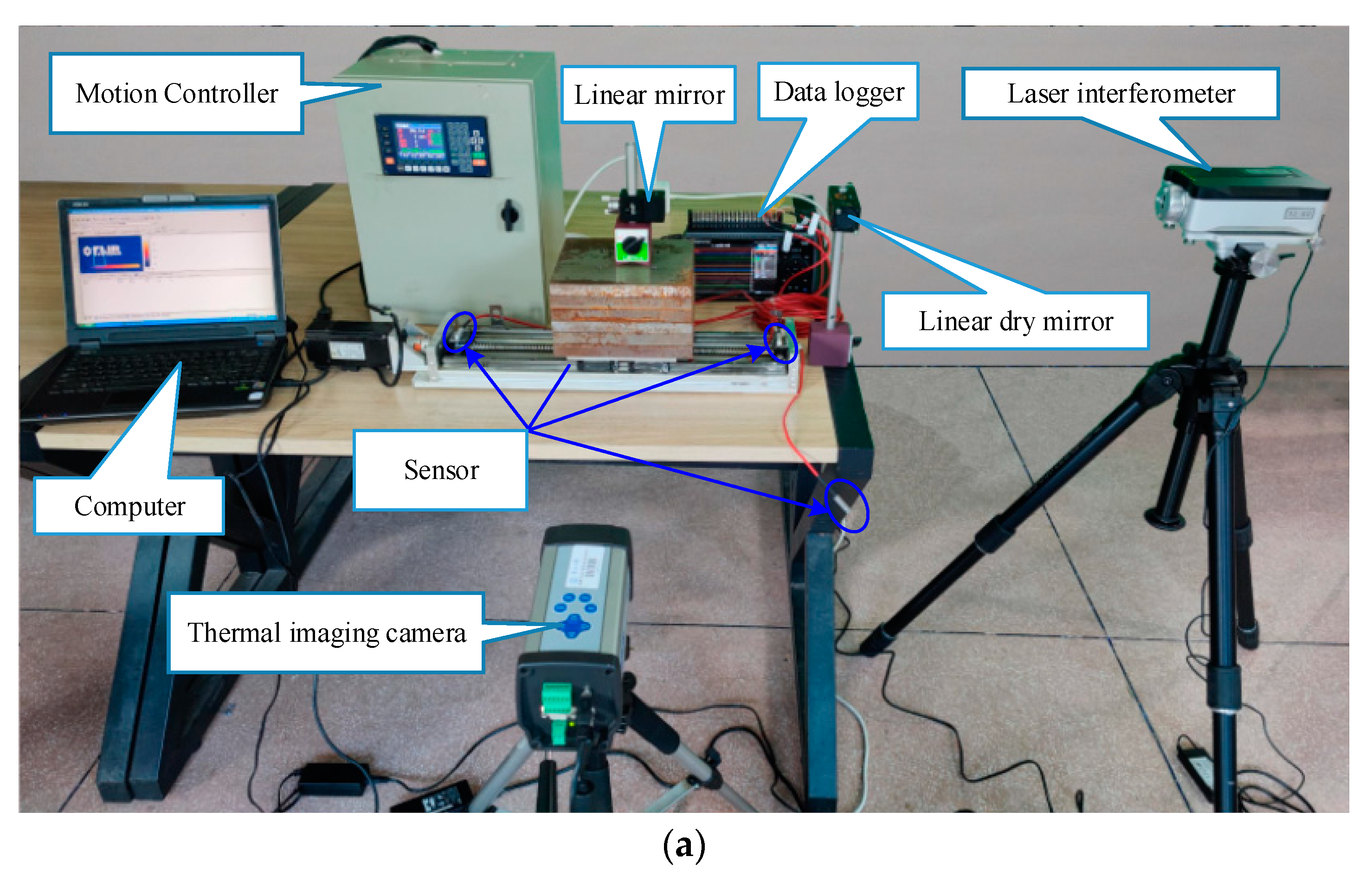
In order to study the thermal characteristics of the ball screw feed system under different working conditions, the experimental equipment is shown in Figure 1. In the experiment, the program was programmed by a motion controller (TC55V) to make the nuts run for 240 min in different operating intervals at a feed rate of 10 m/min. The experimental parameters are shown in Table 3. Due to supporting bearings and bearing seats at both ends of the feed system, the length of the effective stroke is not the full length of the screw shaft, and the actual starting motion coordinate of the ball screw nut pair is at the position of 100 mm. The Pt100-type temperature sensors (with ±0.1 °C accuracy) are used to measure the temperature changes of key points, and the GL840 data logger is used to collect and record the temperature in real-time. The Pt100-type temperature sensor was calibrated before use. The temperature sensor is arranged on the surface of the front bearing (T1) and the rear bearing (T2) by using one component RTV (Room Temperature Vulcanized) Silicone (Ausbong, 189). A sensor is arranged around the test bench to measure the ambient temperature (T3). The specific arrangement position is shown in Figure 2. After the operation, the temperature of the screw shaft is measured by the ThermoVision A40M thermal imaging camera. The uncertainty of the thermal imaging camera is ±2%, and the emissivity is set to 0.95. The temperature distribution of −40~500 °C can be obtained, and the detection accuracy can be as low as 0.08 °C.

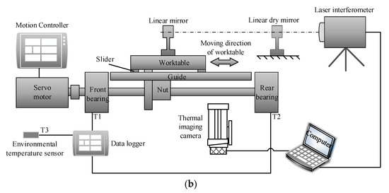
Figure 1.
Experimental equipment and experimental schematic diagram: (a) Experimental equipment; and (b) experimental schematic diagram.
Table 3.
Experimental parameters.
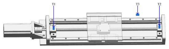
Figure 2.
The layout of the temperature sensors.
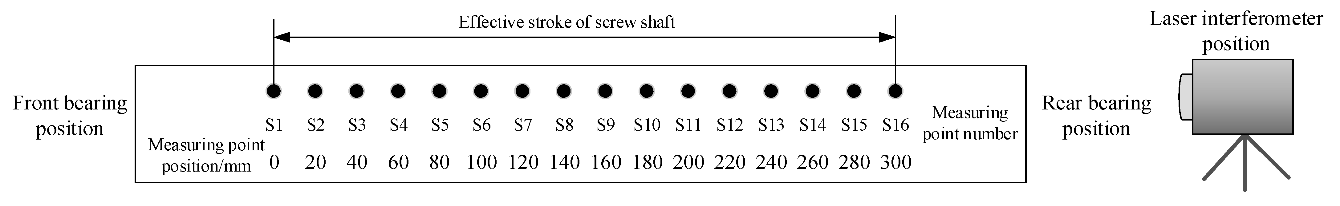
A Renishaw laser interferometer (XL 80, accuracy of 0.5 μm/m) was used to measure the thermal error of the ball screw feed system. First, the positioning error of the feed system in the cold state is measured. Then, by measuring the positioning error in the thermal state under different operating times, the thermal error in the operating state of the ball screw feed system can be obtained through the error separation technology [12,33,34]. During the experiment, 16 points were selected to measure the positioning accuracy to indirectly obtain the thermal error of the ball screw feed system. The distribution of measuring points on the screw shaft is shown in Figure 3. Each point stays for 2 s to ensure the accuracy and stability of data collection.
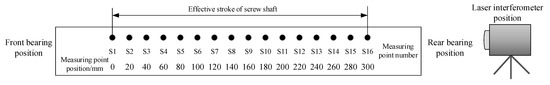
Figure 3.
Distribution of measuring points.
3. Thermal Characteristic Modeling of Ball Screw Feed System
Based on the following assumptions, this paper uses the finite difference method to model the thermal characteristics and analyze the heat transfer of the ball screw feed system [18,19,20]:
- The screw shaft is equivalent to a one-dimensional rod with the same length as the screw shaft;
- The friction heat generated by the reciprocating movement of the nut is uniform, and the heat generated is transferred to the screw shaft in a fixed ratio; the friction heat generated by the rotation of the front and rear bearings is uniform;
- At the same feed rate, the convective heat transfer coefficient is constant;
- When the temperature rise is low, the heat radiation can be ignored;
- The thermal expansion and contraction of the screw shaft are considered to be linear.
3.1. Analysis and Calculation of Boundary Conditions of Ball Screw Feed System
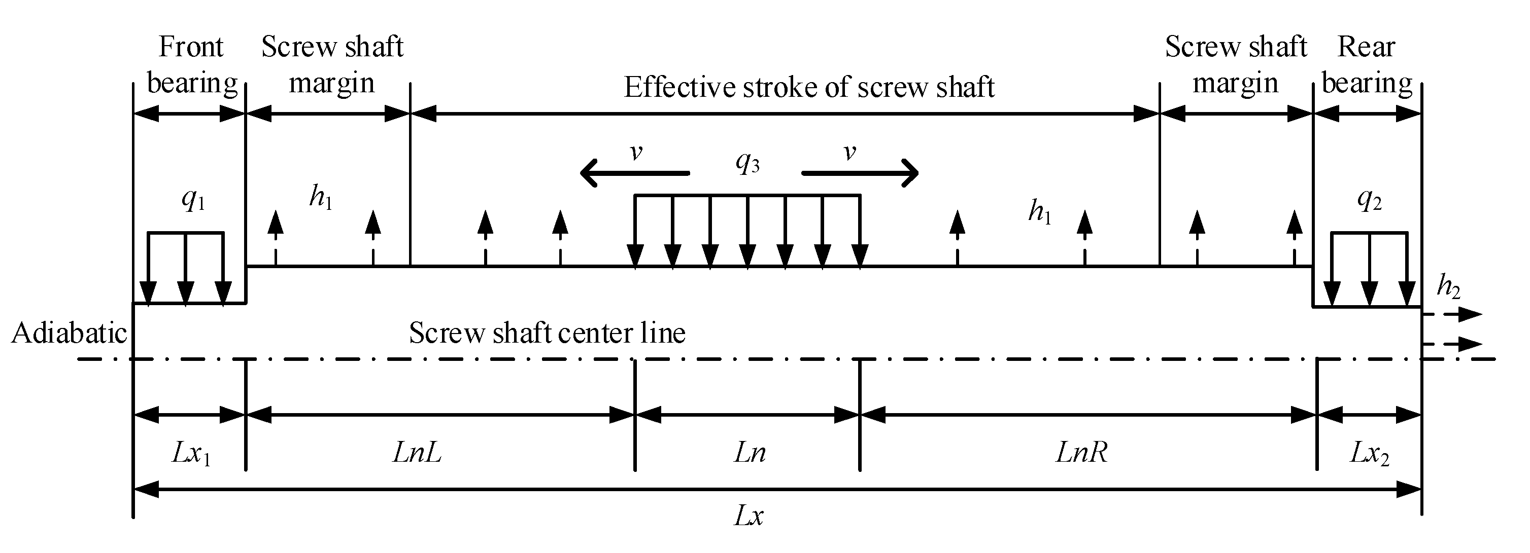
The primary heat sources of the ball screw feed system include servo motors, front bearings, rear bearings, and reciprocating nuts. When the coupling is installed, a flexible diaphragm with an insulating effect is installed between the motor shaft and the screw shaft. The heat generated by the motor is brutal to transfer to the screw shaft. Therefore, the influence of the servo motor on the thermal characteristics of the feed system can be ignored [16]. Replace the nut with a moving heat source and the bearing with a fixed heat source. The thermal characteristic analysis model of the ball screw feed system is shown in Figure 4.
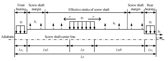
Figure 4.
Thermal characteristics analysis model of ball screw feed system.
The initial boundary condition is as follows:
where Tini represents is the initial temperature of the components of the feed system.
The boundary conditions of the ball screw feed system can be described as follows:
where q1 is the heat generation rate at the front bearing, q2 is the heat generation rate at the rear bearing, and q3 is the heat generation rate at the nut. κ is the thermal conductivity of the screw shaft. Tf is the ambient temperature. h1 is the forced convection heat transfer coefficient on the surface of the screw shaft; and h2 is the convective heat transfer coefficient of the end face of the screw shaft.
3.1.1. Heat Generation of Bearings
According to Harris theory, the heat generated by the bearings is calculated as follows [12,19,35]:
where Qb is the heat generated by the bearing, nb is the bearing speed; Mb is the total friction torques of the bearing; M1 is the friction torque of the bearing caused by the applied load, and Mv is the torque of the bearing caused by viscous friction.
The friction torque M1 caused by the applied load can be obtained as follows:
where f1 is the correlation coefficient with bearing type and load. Fβ is the equivalent load applied to the bearing; dm is the pitch diameter of the bearing; Fa and Fr are the axial loads and radial loads received by the bearing, respectively; α is the contact angle of the bearing.
The friction torque Mv caused by the viscous friction can be obtained as follows:
where f0 is the correlation coefficient with bearing type and lubrication mode, v0 is lubricating oil kinematic viscosity at bearing operating temperature.
3.1.2. Heat Generation of Screw Nut Pair
During the operating of the ball screw nut pair, the heat generated by the friction between the rolling element and the raceway is expressed as follows [36,37]:
where n is the rotation speed of the screw shaft and Mn is the total friction torque of the ball screw nut pair. Md is the driving torque generated to overcome the axial load; Mr is the resistance torque.
The driving torque Md and resistance torque Mr can be obtained as follows:
where Fa and Fp are the axial load and preload of the ball screw nut pair, respectively. Ph is the lead of the screw, η is the transmission conversion efficiency of the ball screw nut pair.
3.1.3. Heat Dissipation
Convection heat transfer coefficient can be obtained as follows [38,39]:
where Nu is the Nusselt number; L is the characteristic length; λair is the thermal conductivity of the surrounding fluid.
According to Equation (10), as long as the Nusselt number Nu is determined, the heat transfer coefficient h can be obtained. There are different calculation methods for the natural convection heat transfer coefficient and forced convection heat transfer coefficient.
During the operation of the feed system, the screw shaft rotates at high speed, which will intensify the heat exchange and heat convection with the surrounding air, which belongs to forced convection heat exchange. The Nusselt number can be defined as follows:
where Re is the Reynolds number; ω is the angular velocity of the screw shaft; Pr is the Prandtl number; and v is the kinematic viscosity of air.
The heat exchange between other parts of the feed system and the air belongs to natural convection heat exchange. The Nusselt number can be defined as follows:
where C is a constant, which is selected according to the heat source and flow pattern; Gr is the Graschev number; g is the acceleration of gravity; β is the expansion coefficient of air; and ΔT is the temperature difference between the air and the parts of the ball screw feed system.
3.2. Construction and Discrete of Heat Conduction Differential Equation for Ball Screw Feeding System
The thermal deformation of the screw shaft is mainly axial thermal deformation, which can be ignored in the radial direction. Therefore, the screw shaft is simplified as a one-dimensional rod, and the differential equation of heat conduction of the ball screw feed system is described as follows:
where ρ is the density of the screw shaft; c is the specific heat capacity of the screw shaft; T(x,t) is the temperature distribution under the action of the heat source of the screw shaft; and S is the system heat source term.
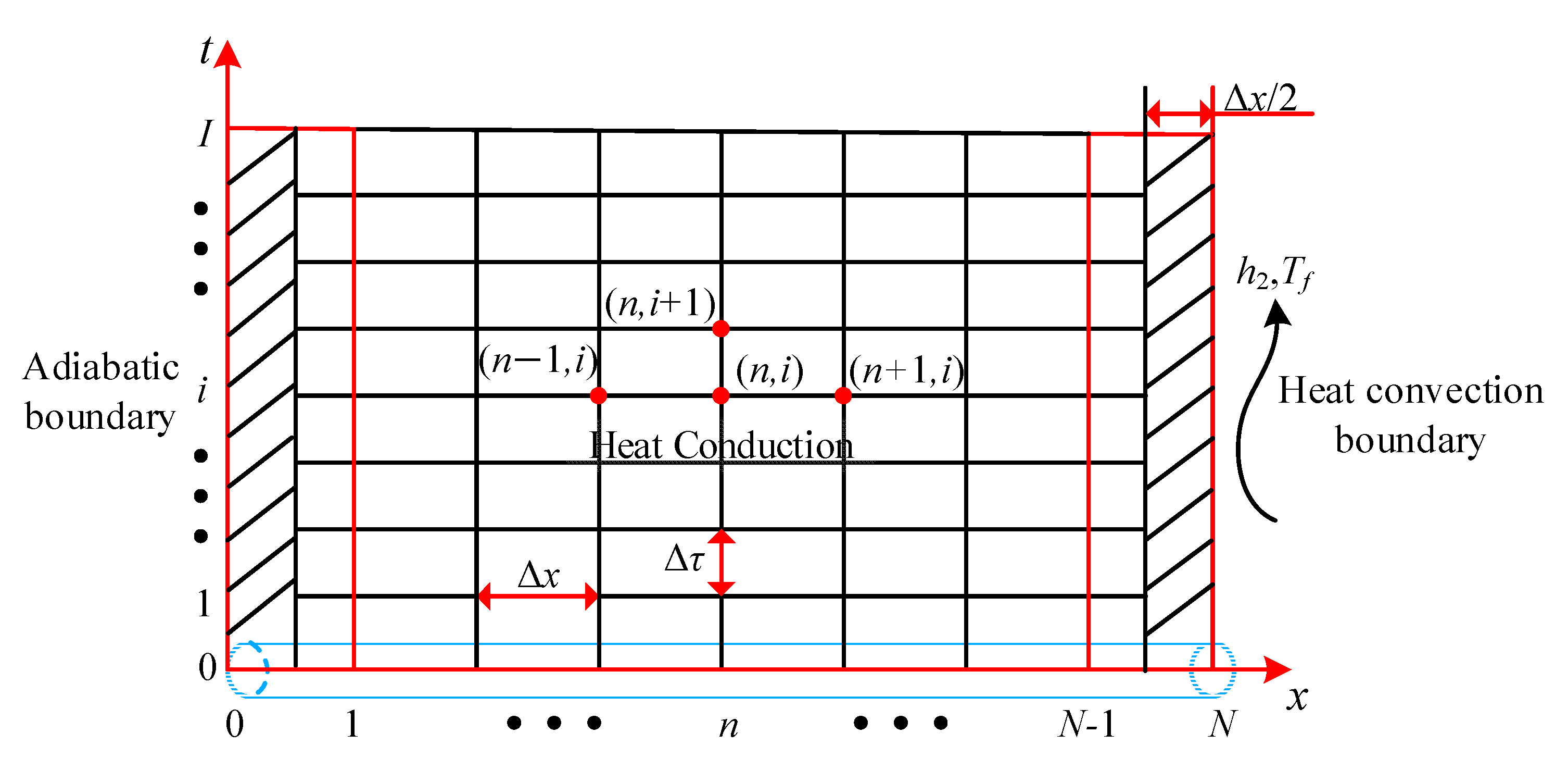
In order to solve the differential equation of heat conduction, the screw shaft is discretized into a grid according to the time step Δτ and the space step Δx, as shown in Figure 5. The intersection point in the graph, such as (n, i), represents a specific “time-space” node position. In order to facilitate the calculation of the node temperature value, is used to represent the current temperature of the node, and is used to represent the temperature of the node at the next time.
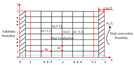
Figure 5.
Schematic diagram of the “time-space” dispersion of the screw shaft.
The length of the screw shaft is divided into N equal parts, and (N + 1) spatial nodes are obtained in the length direction. The total length L can be described as follows:
The total time is divided into I equal parts. The total time t is described as follows:
Equation (15) can be rewritten base on the explicit difference method. The first-order and second-order differential terms can be described as follows:
The discrete equation of the inner node is described as follows:
The right side of the screw shaft is exposed to the air and exchanges heat with the air. The surface heat transfer coefficient is h2, the air temperature is Tf, the boundary node is N, and the node N represents a micro-element body with a width of Δx/2. The difference equation of the surface grid is obtained using the energy conservation conditions of adjacent nodes, and the discrete equation of convective boundary nodes is described as follows:
The front bearing end of the screw is set as an adiabatic boundary condition. For adiabatic boundary conditions, the derivation process is similar to convective boundary conditions, and only the convective heat transfer at the convective boundary is zero. The nodal dispersion equation of the front bearing end adiabatic boundary condition is described as follows:
According to the inner node discrete Equation (21) and the boundary node discrete Equations (23) and (25), the discrete equations of the feed system at different node positions can be described as follows:
According to Equation (26), it can be seen that as long as the initial temperature distribution is known, the temperature distribution at other times can be obtained sequentially. However, the selection of space step size Δx and time step size Δτ follows the second law of thermodynamics, and the following stability conditions must be met:
According to Equation (27) and combined with structural and material parameters, the space step Δx and time step Δτ can be determined. Finally, the space node N = 200 and the space step Δx = 2.5 mm are selected. When selecting the time step Δτ, it is necessary to ensure that the stability conditions are met, and the time step Δτ must be as small as possible. Finally, the time step Δτ = 0.25 s is selected.
3.3. Application of Nut Moving Heat Source
The heat generated by the ball screw nut pair comes from the friction between the rolling element and the raceway, and the friction heat comes from the friction power consumption. Regardless of the distribution of the heat source model function, the total frictional heat in the contact area is the same [40]. Therefore, the heat generated by the nut under different working conditions is replaced by a fixed heat value. Moreover, the functional relationship between the nut heat source position and the operating time is established to simulate the effect of nut reciprocating motion on the screw shaft. The application process of nut moving heat source is as follows:
- The total length L of the screw shaft, the length of the nut Ln and the effective stroke of the screw shaft are determined. The length of the nut Ln is the length of the moving heat source, and the maximum operating interval of the nut moving heat source is the effective stroke range.
- The position of the nut heat source is determined by the position of the centerline Lncenter of the nut length. Establish the relationship between the nut edge, the centerline of the nut length, and the nut length as follows:
- 3.
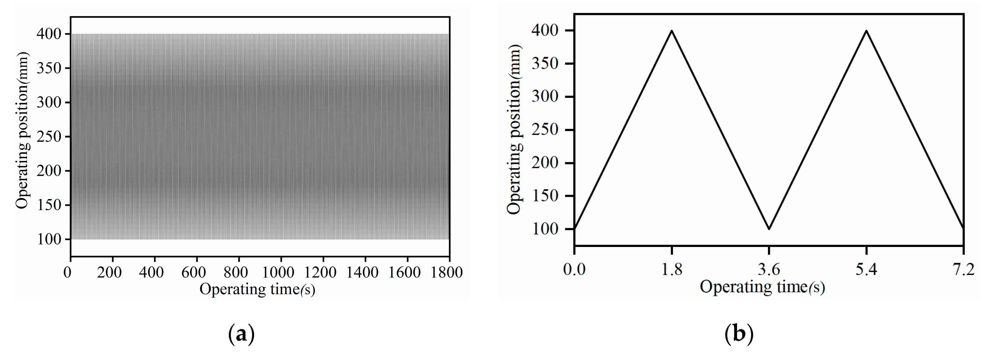
- The operating interval, operating time, and feed rate are determined to match the actual working conditions. The defined nut heat source operating time is the total time of the feed system, which is the same as the actual working process of the feed system. When the movement of the ball screw nut pair is stopped, the heat will no longer be generated by the feed system. For example, in the operating interval of 100~400 mm and operating at a feed rate of 10 m/min for the 1800 s, the function diagram between the nut heat source position and operating time during operating is shown in Figure 6a. Due to the fast operating speed and short operating interval, the function diagram is very dense. Figure 6b is an enlarged diagram of the function between the nut heat source position and the operating time. For different operating intervals and feed rates, the above parameters and diagrams must be recalculated and drawn.
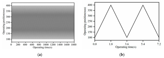 Figure 6. Function diagram: (a) The function diagram between the nut heat source position and operating time; (b) enlarged diagram of the function between the nut heat source position and the operating time.
- 4.
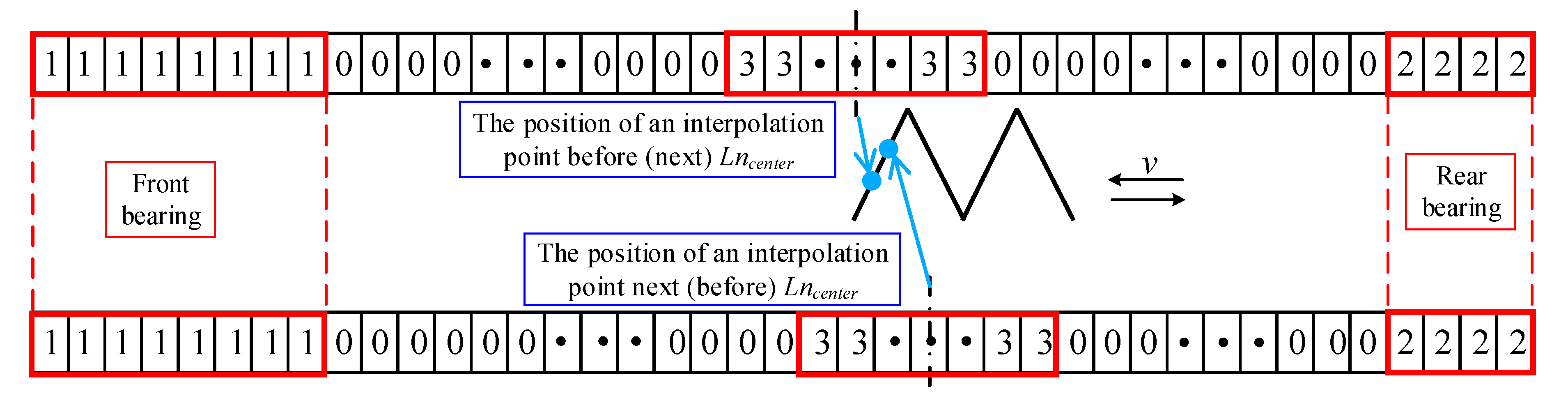
- The divided grid is parameterized, and the heat generation rate of the corresponding grid position is determined. The front bearing area is set to “1”, and the front bearing heat generation rate q1 is applied; the rear bearing area is set to “2”, and the heat generation rate q2 of the rear bearing is applied. The area is centered on the nut center Lncenter, the left boundary is Ln1, and the right boundary is Ln2, which is set to “3”, and the nut heat generation rate q3 is applied. The remaining positions are set to “0”, and convective heat source terms are applied. The movement of the nut heat source at different positions is realized by interpolation function interp1. According to the established functional relationship between the nut heat source position and the operating time, the different positions of the nut center Lncenter at different times are obtained by interpolation calculation. The positions “1” and “2” of the front and rear bearings remain unchanged, the new interpolation position of the nut heat source centered on Lncenter is set to “3”, and the remaining positions are set to “0”. The same method is used to reach each interpolation position so that the movement of the nut heat source at each position can be simulated. The schematic diagram of the nut moving heat source application is shown in Figure 7.
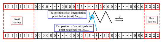 Figure 7. Schematic diagram of applying nut moving heat source.
3.4. Solution Process
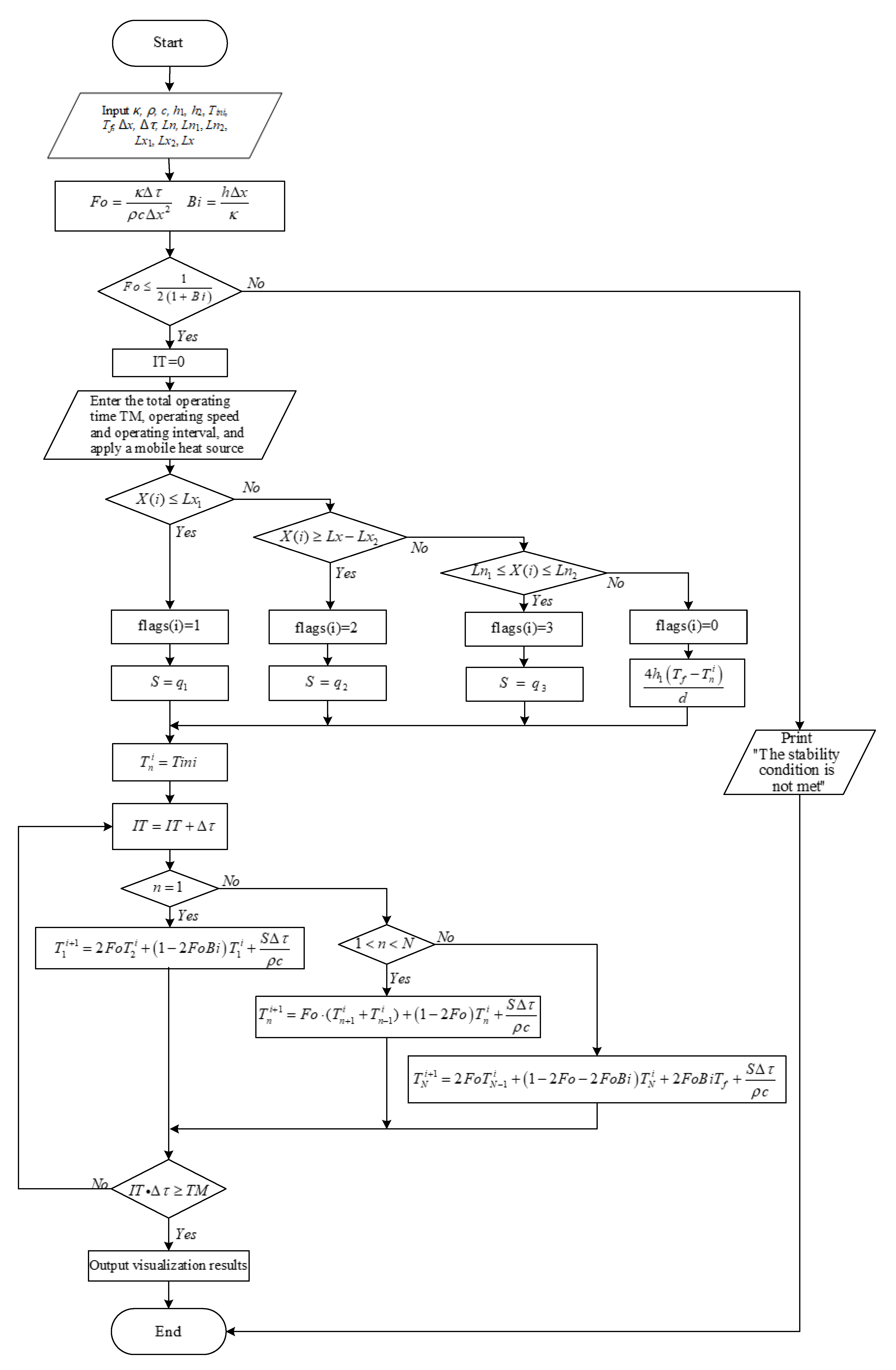
In this paper, the differential equation of heat conduction of the ball screw feed system is discretized into a finite difference scheme. MATLAB software is used to iteratively solve the temperature distribution of the screw shaft under different working conditions. The process is as follows:
- Initialization. Material parameters, size parameters, and initial conditions are input. The ambient temperature Tf and the initial temperature Tini of the components are both 22 °C;
- Stability is determined according to the selected time step and space step;
- The total operating time TM, operating interval, and operating rate are determined. According to the application step of the mobile heat source, the mobile heat sources are applied;
- The loading type of S is determined by the location of x(i). The heat source is applied to the corresponding position, and the boundary values applied are shown in Table 4;
Table 4. Load values of boundary conditions.
- According to the node’s location, the node type is determined as an internal node, adiabatic boundary node, or convective boundary node. Moreover, through the corresponding discrete equation, the temperature value of each space node is calculated.
- Judge whether the total operating time TM is reached. If the total time is reached, exit the loop, and the obtained temperature data as a visualization result are output. If the total time is not reached, return to step (5) to continue running until the total operating time is reached.
According to the above solving steps, a program is written to solve the problem. The solution process is shown in Figure 8.
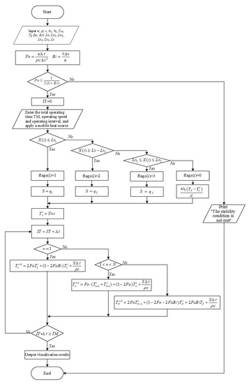
Figure 8.
The finite difference method to solve the temperature distribution flow chart of the ball screw feed system.
3.5. Establishment of Thermal Error Model of Ball Screw Feed System
The installation mode of one end fixed and the other end supported is adopted by the support and positioning mode of the ball screw feed system studied. The fixed support end is considered to be immovable both axially and radially. The supporting end is considered immovable in the radial direction but has no restriction in the axial direction and can extend freely. The relationship between temperature change and thermal expansion is established based on the predicted temperature distribution of the ball screw feed system under different working conditions. The screw shaft is divided into several sufficiently small units. As it is small enough, there is no temperature gradient inside, and it can be considered that it is thermally uniform. The thermal error model for each divided unit is as follows:
where αT is the thermal expansion coefficient.
The thermal error of the ball screw feed system is the accumulation of the thermal error of all the equally divided units, as follows:
4. Simulation Results and Verification
4.1. Analysis of Temperature Field in Different Working Conditions
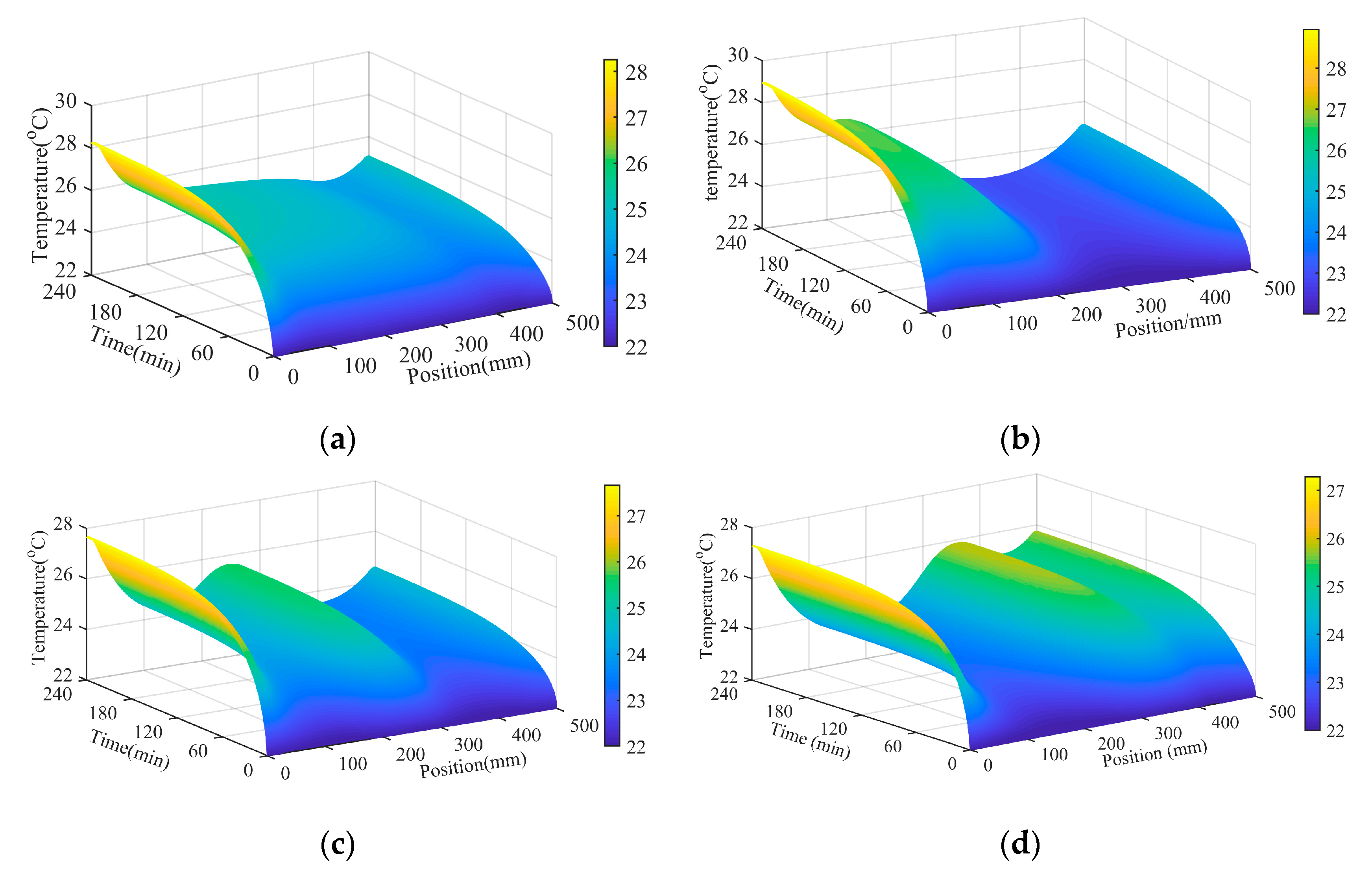
Based on the established thermal characteristic model of the ball screw feed system, the temperature field of the ball screw feed system is analyzed. The simulated working conditions are shown in Table 3. The simulated temperature distributions of the feed system under different operating conditions are obtained, as shown in Figure 9. It can be seen that the temperature gradient changes obviously in the working area of the screw shaft; that is, the temperature changes significantly in the front bearing area, the rear bearing area, and the nut operating interval. The temperature change trend of the screw shaft operating interval is closely related to the working conditions.

Figure 9.
Temperature simulation results of the ball screw feed system under different working conditions: (a) working condition 1; (b) working condition 2; (c) working condition 3; and (d) working condition 4.
According to Figure 9a, it can be seen that when the operating interval is 100~400 mm, after reaching the steady-state, the temperature distribution in the operating interval is uniform, and there is no “bulging phenomenon” like other operating intervals. That is because the operating interval is long, and the screw shaft can get a sufficient heat dissipation time after the nut heat source passes. Moreover, the heat generated by the bearing and the nut in the operating interval diffuses into the margin of the screw shaft, increasing the temperature in the margin of the screw, and the temperature difference with the operating interval is not significant, so there will be no “bulging phenomenon.” According to Figure 9b–d, it can be seen that when the operating interval is short, the temperature distribution within the operating interval will appear “bulging phenomenon.” As the operating interval is short, the friction frequency between the rolling elements and the raceway in the operating interval will increase. The cooling time of the screw shaft in the operating interval is short, and the heat cannot be dissipated in time. Eventually, the temperature in the operating interval has increased significantly locally, and the “bulging phenomenon” in the temperature distribution diagram appears.
Comparing Figure 9b–d shows that the closer the nut heat source is to the bearing heat source at both ends, the higher the temperature of the bearing area and the operating interval after reaching a steady state. The heat generated by the bearing and the nut diffuses to the surrounding area and affects each other, causing the temperature to rise. Compared with Figure 9b,d, it can be seen that even if the nut heat source value is the same, the distance from the front bearing and the rear bearing is the same. However, the temperature distribution under the two conditions is only similar to the growing trend. The shape of the temperature distribution in the operating interval is different. That is because the structures and installation of the front and rear bearing are different.
In summary, to reduce the influence of temperature on the thermal deformation of the feed system, it is necessary to consider the influence of the operating interval of the worktable on the accuracy of the feed system during processing. During installation and use, the operating interval of the nut heat source should be as far away as possible from the bearing heat source at both ends, and the operating area during processing should be considered when the machine tool is preheated.
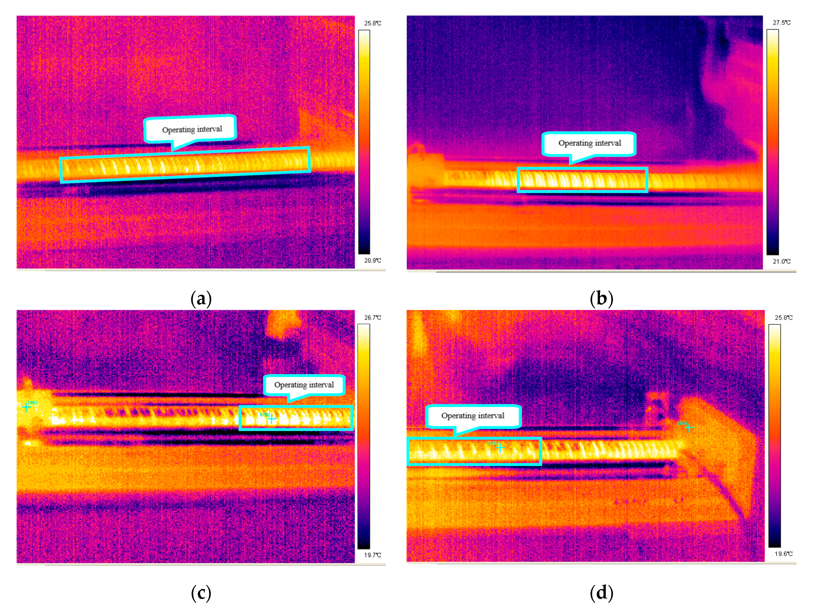
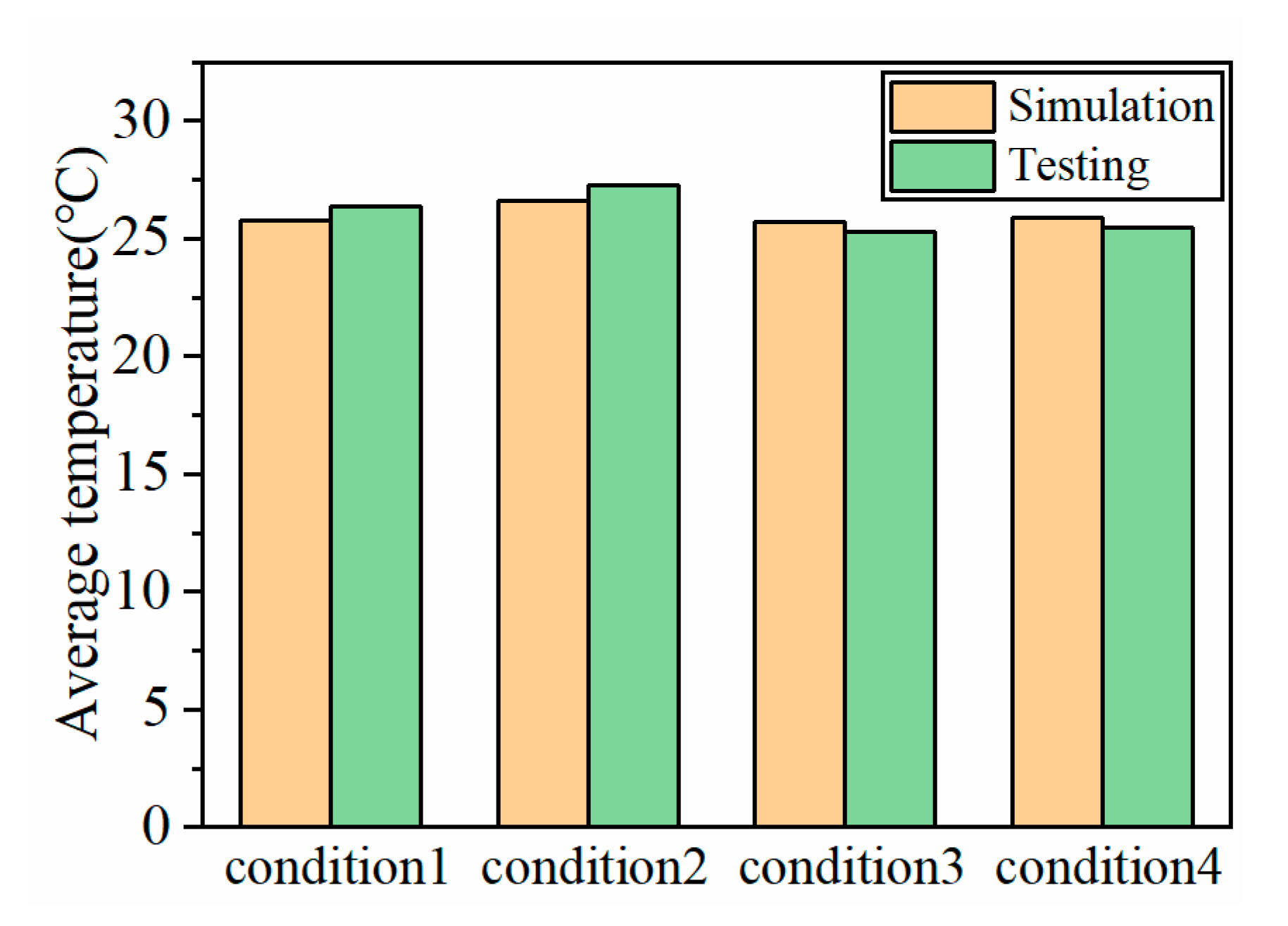
After the operation is over, the temperature distribution of the ball screw feed system under different working conditions is obtained by a thermal imaging camera, as shown in Figure 10. Comparing Figure 9 and Figure 10 shows that the temperature distribution in the operating interval simulated by the finite difference method considering the nut moving heat source is in good agreement with the temperature distribution measured by the experiment. The comparison between the simulated average temperature of the operating interval and the experimental average temperature under different working conditions is shown in Figure 11. It can be seen that the error is less than 11.4%, which proves the effectiveness of the method used. The cause of the error is that the convective heat transfer coefficient between the screw shaft and the air is considered constant in the simulation. The convective heat transfer coefficient will change with the change of temperature in the actual working process [40,41]. Moreover, the airflow speed around the screw shaft and the lubrication and cooling of the screw shaft will affect the steady-state temperature of the screw shaft.
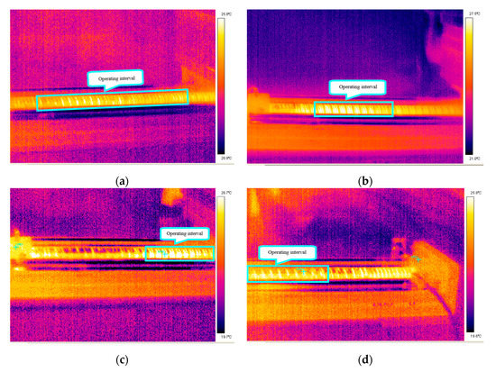
Figure 10.
Temperature experimental results of the ball screw feed system under different working conditions: (a) working condition 1; (b) working condition 2; (c) working condition 3; and (d) working condition 4.
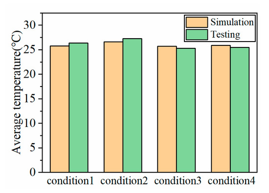
Figure 11.
Comparison of simulation results and experimental results of average temperature in the operating interval.
4.2. Temperature Analysis of Different Nodes in Different Working Conditions
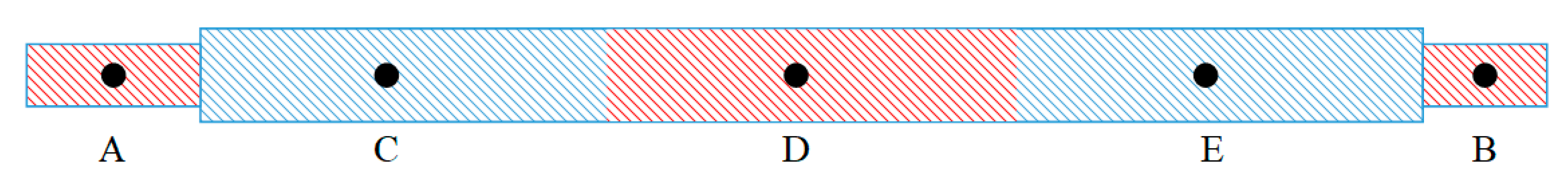
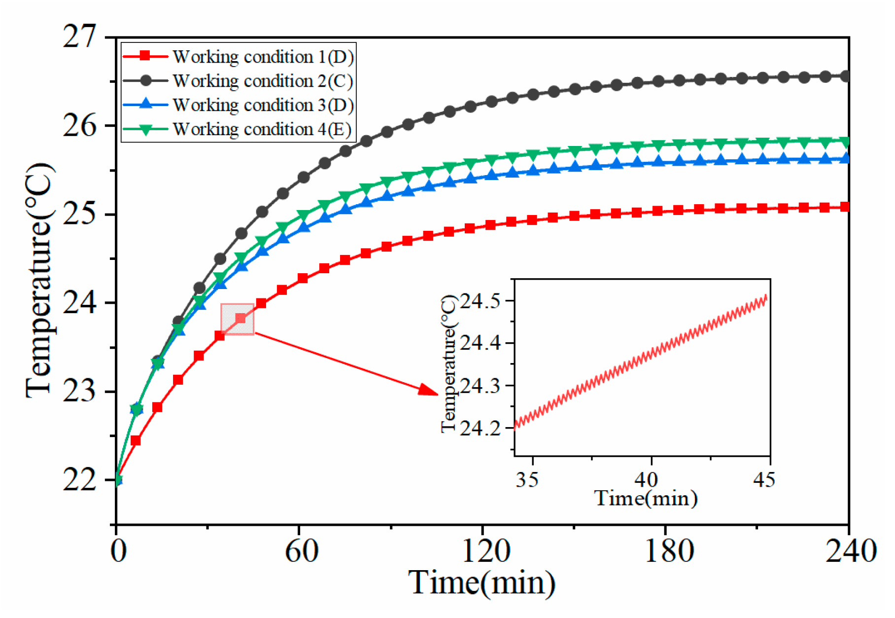
Select the midpoint of the heat source area on the surface of the screw shaft to represent the area’s temperature and observe the temperature change rules at different nodes. Node A represents the front bearing position, and node B represents the rear bearing position. Node C represents the position in the operating interval of 100 to 200 mm, node D represents the position in the operating interval of 100 to 400 mm and 200 to 300 mm, and E represents the position in the operating interval of 300 to 400 mm. The node position is shown in Figure 12. The temperature variation curves of nodes in the operating interval under different working conditions are shown in Figure 13.
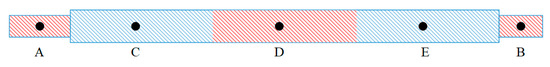
Figure 12.
Location of temperature nodes.
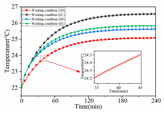
Figure 13.
Nodes temperature change in operating interval under different working conditions.
According to Figure 13, it can also be seen that the temperature changes of the operating interval nodes are different. When operating under working condition 1, due to the long-operating interval, the operating interval of the screw shaft has sufficient heat dissipation time, so the final steady-state temperature is the lowest. When operating under condition 2, the operating interval is close to the front bearing. The heat generated by the front bearing is large, and the heat will be transmitted to the operating interval, which increases the temperature of the operating interval. Moreover, in working condition 2 operation, due to the short operation interval, the heat dissipation time of the screw shaft operation interval is insufficient, increasing the temperature of the operation interval. When operating under working condition 4, since the operating interval is close to the rear bearing, the heat generated will be transmitted to the rear bearing position, making the temperature at the rear bearing further increase on the original basis. When operating under working condition 3, the bearing heat source has little influence due to the long distance from the two ends of the bearing. Therefore, the steady-state temperature is lower than the steady-state temperature at working condition 2 and working condition 4.
Take working condition 1 as an example to observe the changing trend of node temperature in the operating interval. According to Figure 13, it can be seen that the temperature curve of node D in the operating interval shows an upward trend as a whole, but there will be regular fluctuations. The nut heat source applied is a mobile heat source, which reciprocates in the operating section. When the nut heat source moves to the node D position, the temperature rises; when the nut heat source leaves node D and moves to the next position, the node D position will convectively exchange heat with the air to reduce the temperature. Therefore, the temperature change curve of node D is a curve with an upward trend and regular fluctuations as a whole.
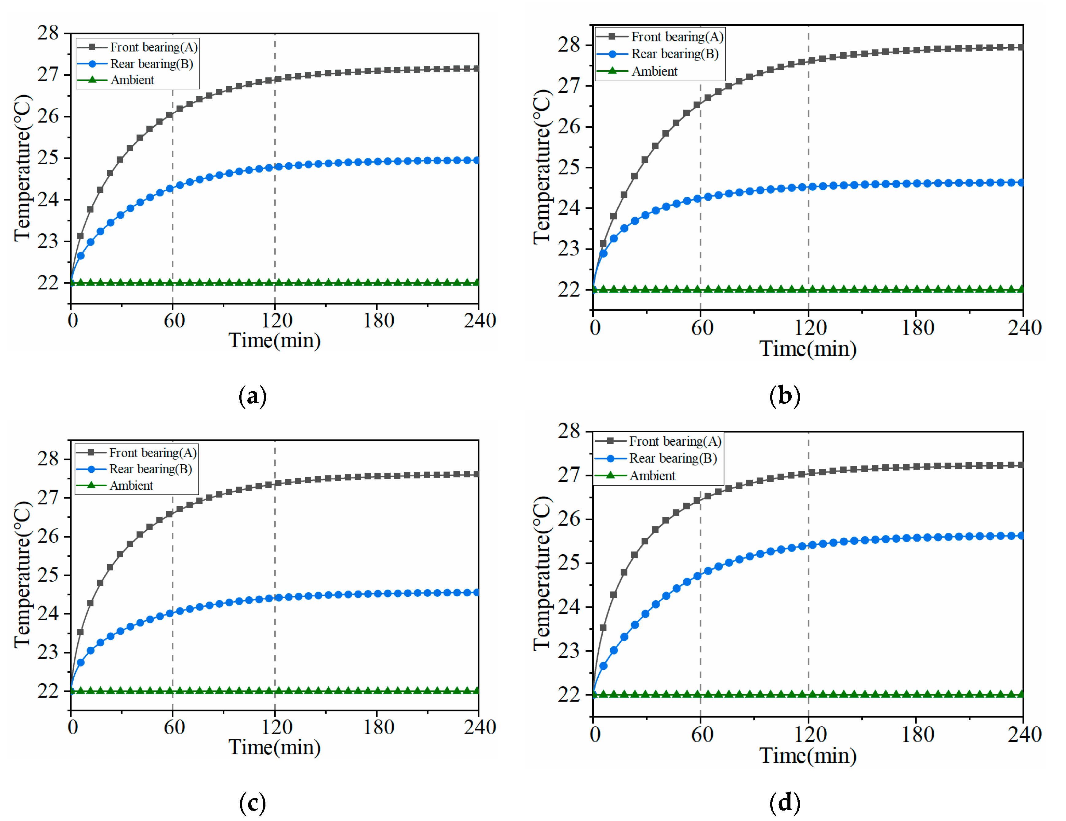
The temperature curves of the front bearing position node A and the rear bearing position node B with time are shown in Figure 14. It can be seen that before 60 min, the heat generated by the friction of each component makes the temperature of each node rise rapidly, and the temperature rise reaches 80% of the steady-state temperature. After 120 min, the heat generated by the component is gradually equal to the heat dissipated to the environment. The temperature rise rate gradually slows down to reach a steady state.
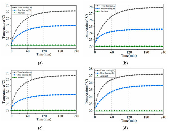
Figure 14.
Simulation results of the node temperature of the ball screw feed system under different working conditions: (a) working condition 1; (b) working condition 2; (c) working condition 3; and (d) working condition 4.
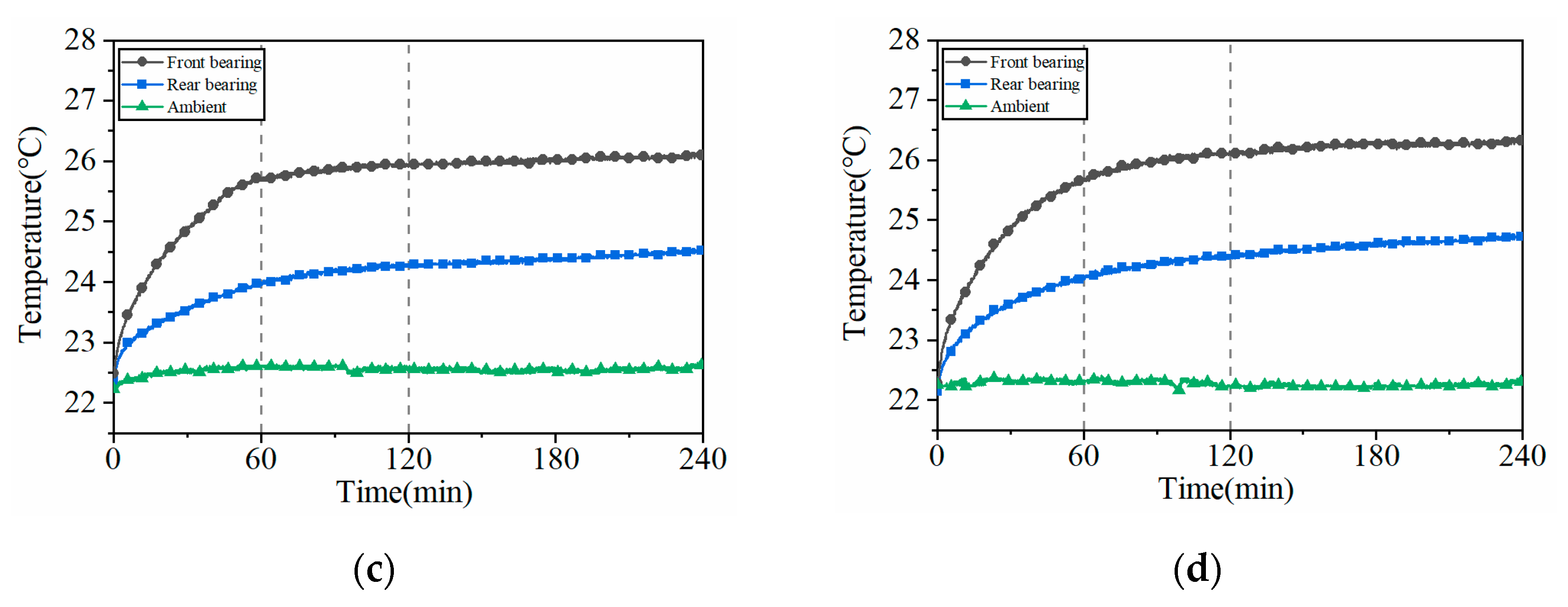
The temperature sensors arranged at the key points can get the temperature change curves of the key points under different working conditions, as shown in Figure 15. It can be seen that the temperature rise trend of each component measured in the experiment is consistent with the simulated temperature rise trend in Figure 14, showing good consistency. The temperature rises rapidly in the first 60 min, and the temperature is unchanged for 120 min to reach a steady state. Since the temperature sensor cannot be installed on the screw shaft, the temperature data of the operating interval are not measured in the experiment.
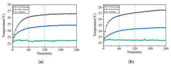

Figure 15.
Experimental results of node temperature of the ball screw feed system under different working conditions: (a) working condition 1; (b) working condition 2; (c) working condition 3; and (d) working condition 4.
Comparing Figure 14 and Figure 15, it can be seen that the steady-state temperature of the bearing obtained by the simulation is higher than the steady-state temperature of the bearing tested in the experiment. The nodes selected in the simulation are all on the screw shaft, and the test points selected in the experiment are on the bearing seat surface. Due to contact thermal resistance [42,43,44], the conduction of temperature at the junction will cause temperature loss, resulting in an error in temperature results. Moreover, the environmental temperature is difficult to maintain as constant during the experiment. In the simulation, the ambient temperature is considered constant, which will also cause errors in the temperature results. In addition, the influence of bearing lubricant on the cooling effect was not considered during the simulation process, which would make the simulated temperature higher than the experimentally measured temperature.
4.3. Analysis of Thermal Error in Different Working Conditions
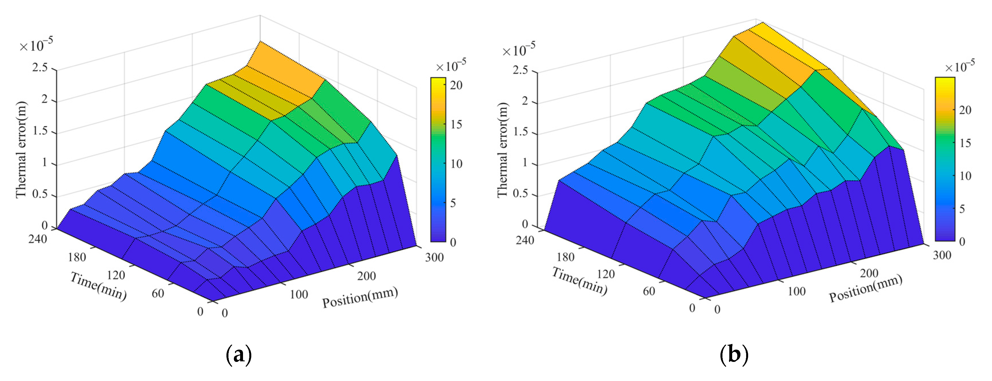
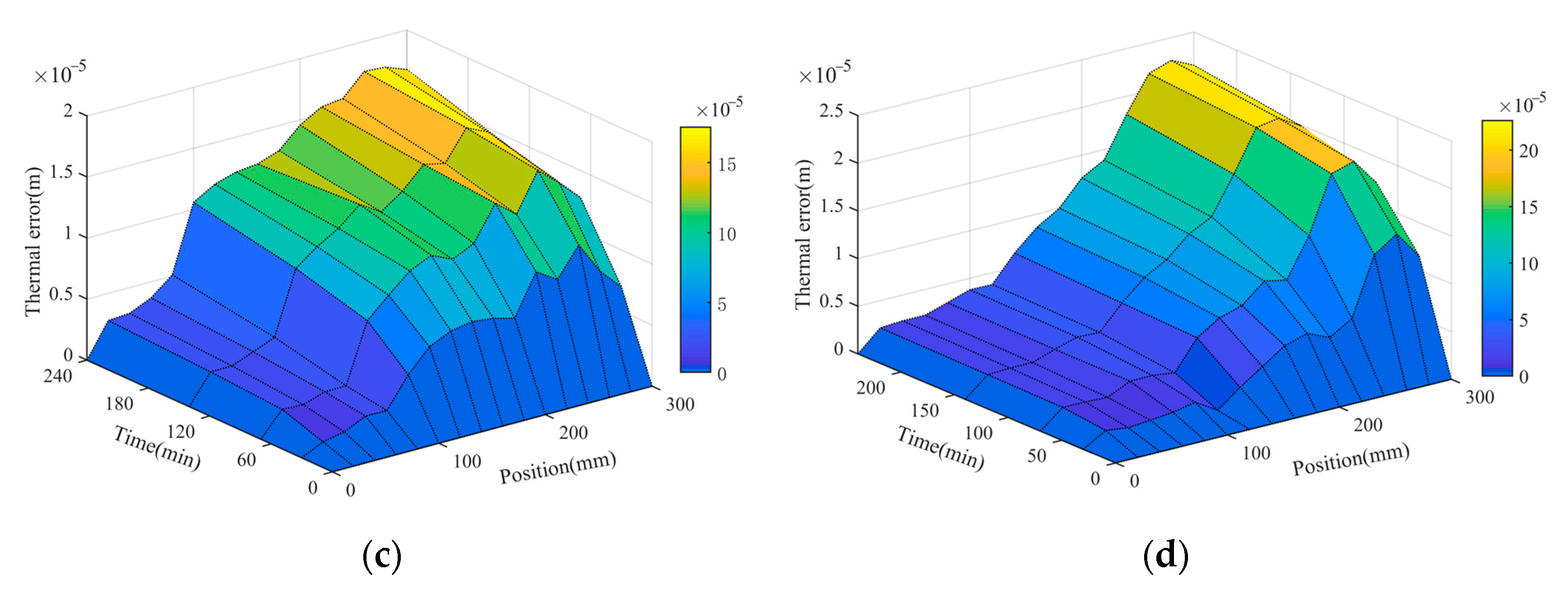
The established error model is used to calculate the thermal error of the ball screw feed system under different working conditions. The thermal error simulation results of the ball screw feed system under different working conditions are obtained in Figure 16. According to Figure 16, it can be seen that as the operating time increases, the larger the thermal error, and the further away from the front bearing position, the larger the thermal error. Due to the installation method of the screw shaft, the screw shaft expands to the end without axial restraint after being thermally expanded, causing the thermal error of each unit to accumulate to the rear bearing end. As a result, the thermal error becomes larger and larger farther away from the front bearing end.
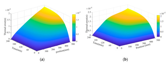
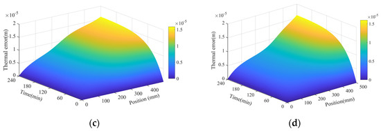
Figure 16.
Simulation results of thermal error of ball screw feed system under different working conditions: (a) working condition 1; (b) working condition 2; (c) working condition 3; and (d) working condition 4.
According to Figure 16, it can also be seen that the thermal error changes within the operating interval are more evident than those in the non-operating interval, and the thermal error results within the operating interval have “bulging” characteristics in the operating interval. According to Figure 9, the temperature in the operating interval is significantly higher than the non-operating interval, so the thermal error in the operating interval has changed significantly. The thermal error result has a “ bulging” characteristic.
The thermal error distribution of the ball screw feed system measured in the experiment is shown in Figure 17. Comparing Figure 16 and Figure 17, it can be seen that the thermal error simulation results obtained by the established thermal error model are consistent with the laws presented by the experimental thermal error results. The comparison of the thermal error simulation results and the thermal error experimental results of the bearing end is shown in Figure 18. It can be seen that the maximum relative error between the thermal error simulation result and the experimental result is 16.4%. The feed system measured in the experiment has a nonlinear geometric error. The thermal error is superimposed on the initial geometric error, and the distribution of geometric error will affect the thermal error. In the process of simulating thermal error, it is considered that there is no geometric error at the initial time. Therefore, there are errors between the simulation results and experimental results of thermal error. The thermal error distribution of the feed system cannot be measured directly and timely using the laser interferometer, which will lead to the error of the thermal error results obtained in the experiment.


Figure 17.
Experimental results of thermal error of ball screw feed system under different working conditions: (a) working condition 1; (b) working condition 2; (c) working condition 3; and (d) working condition 4.
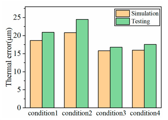
Figure 18.
Comparison of thermal error simulation results and thermal error experimental results.
According to Figure 16 and Figure 17, it can be seen that the thermal error distribution in different operating intervals and different operating times will be different. At the beginning of the operation, there will be apparent changes near the curve of the heat source, showing a multi-section spline curve. In the later period of operation, the curve shows a linear curve. Therefore, when the thermal error is compensated, different compensation methods should be adopted in different operating intervals and different operating times.
5. Conclusions
In this paper, the movement of the nut is regarded as the movement of the heat source, and the finite difference method is used to simulate the temperature field and thermal error of the ball screw feed system under different working conditions. The experimental results of the temperature field are obtained by the temperature sensors and thermal imaging camera. The thermal error experimental results were indirectly obtained by using the laser interferometer. In order to reduce the gap between simulation and actual operation, the ball screw is parameterized, and the interpolation function is used to interpolate the relationship between the position of the nut heat source and the operating time to realize the movement of the nut heat source at each position. The simulation temperature results and thermal error results were compared with the experimental temperature results and thermal error results, showing good consistency. The results show that the influence of operation interval on the positioning accuracy of the feed system should be considered in the actual operation process. In order to reduce the influence of temperature, the operating interval of the nut heat source should be as far away from the bearing heat source at both ends as possible during installation and use. The operating interval should be selected as far as possible in the middle range of the effective stroke of the screw shaft and should be considered in the preheating of CNC machine tools. When compensating for the thermal error of CNC machine tools, different compensation methods should be adopted at different operating intervals and different operating times. The thermal characteristics modeling method of the ball screw feed system proposed in this paper is closer to the actual moving process of the nut, narrows the gap between the simulation and the actual moving process, and has substantial application value for accurately obtaining the temperature field of the feed system.
Author Contributions
Conceptualization, H.L. and Y.Z.; methodology, H.L.; software, R.P. and Z.R.; validation, H.L., R.P. and Z.R.; formal analysis, H.L.; investigation, H.L., R.P. and Z.R; resources, Y.Z.; data curation, Y.Z.; writing—original draft preparation, H.L.; writing—review and editing, H.L., Z.R. and R.P.; supervision, H.L. and Y.Z.; funding acquisition, Y.Z. All authors have read and agreed to the published version of the manuscript.
Funding
This research was funded by Key-Area Research and Development Program of Guangdong Province, grant number 2020B090928001. This research was funded by Liaoning Provincial Department of Education 2021 Scientific Research Funding Project, grant number LJKZ0001.
Institutional Review Board Statement
Not applicable.
Informed Consent Statement
Not applicable.
Data Availability Statement
Not applicable.
Conflicts of Interest
The authors declare no conflict of interest. The funders had no role in the design of the study; in the collection, analyses, or interpretation of data; in the writing of the manuscript, or in the decision to publish the results.
References
- Mayr, J.; Jedrzejewski, J.; Uhlmann, E. Thermal issues in machine tools. Cirp. Ann. Manuf. Technol. 2012, 61, 771–791. [Google Scholar] [CrossRef] [Green Version]
- Bryan, J.B. International Status of Thermal Error Research. CIRP Ann. 1990, 39, 645–656. [Google Scholar]
- Liu, K.; Liu, Y.; Sun, M.; Wu, Y.; Zhu, T. Comprehensive thermal compensation of the servo axes of CNC machine tools. Int. J. Adv. Manuf. Technol. 2016, 85, 2715–2728. [Google Scholar] [CrossRef]
- Li, B.; Tian, X.; Zhang, M. Thermal error modeling of machine tool spindle based on the improved algorithm optimized BP neural network. Int. J. Adv. Manuf. Technol. 2019, 105, 1497–1505. [Google Scholar]
- Liu, D.S.; Lin, P.C.; Lin, J.J. Effect of environmental temperature on dynamic behavior of an adjustable preload double-nut ball screw. Int. J. Adv. Manuf. Technol. 2019, 101, 2761–2770. [Google Scholar]
- Heisel, U.; Koscsák, G.; Stehle, T. Thermography-Based Investigation into Thermally Induced Positioning Errors of Feed Drives by Example of a Ball Screw. CIRP Ann. 2006, 55, 423–426. [Google Scholar] [CrossRef]
- Jedrzejewski, J.; Kwasny, W. Knowledge base and assumptions for holistic modelling aimed at reducing axial errors of complex machine tools. J. Mach. Eng. 2013, 13, 7–25. [Google Scholar]
- Ahn, J.Y.; Chung, S.C. Real-time estimation of the temperature distribution and expansion of a ball screw system using an observer. Proc. Inst. Mech. Eng. B J. Eng. Manuf. 2004, 218, 1667–1681. [Google Scholar]
- Xiang, S.; Zhu, X.; Yang, J. Modeling for spindle thermal error in machine tools based on mechanism analysis and thermal basic characteristics tests. Proc. Inst. Mech. Eng. C J. Mech. Eng. Sci. 2014, 228, 3381–3394. [Google Scholar] [CrossRef]
- Zivkovic, A.; Zeljkovic, M.; Tabakovic, S. Mathematical modeling and experimental testing of high-speed spindle behavior. Int. J. Adv. Manuf. Technol. 2015, 77, 1071–1086. [Google Scholar]
- Uhlmann, E.; Hu, J. Thermal modeling of an HSC machining centre to predict thermal error of the feed system. Prod. Eng. Res. Devel. 2012, 6, 603–610. [Google Scholar]
- Yang, J.; Zhang, D.; Mei, X. Thermal error simulation and compensation in a jig-boring machine equipped with a dual-drive servo feed system. Proc. Inst. Mech. Eng. B J. Eng. Manuf. 2015, 229, 43–63. [Google Scholar] [CrossRef]
- Mao, X.; Mao, K.; Du, Y. Analysis of the Thermal Characteristics of Machine Tool Feed System Based on Finite Element Method. Adv. Technol. Design. Mech. Aeronaut. Eng. 2017, 234, 012013. [Google Scholar]
- Horejš, O. Thermo-Mechanical Model of Ball Screw with Non-Steady Heat Sources. In Proceedings of the 2007 International Conference on Thermal Issues in Emerging Technologies: Theory and Application, Cairo, Egypt, 3–6 January 2007; pp. 133–137. [Google Scholar]
- Cao, J.; Li, L.; Liu, Y.; Sun, J. Research on Thermal Characteristics of High Speed Hollow Ball Screw in Different Working Conditions. Modular Mach. Tool Autom. Manuf. Tech. 2011, 3, 30–37. [Google Scholar]
- Liu, J.L.; Ma, C.; Wang, S.L. Thermal boundary condition optimization of ball screw feed drive system based on response surface analysis. Mech. Syst. Signal. Process. 2019, 121, 471–495. [Google Scholar] [CrossRef]
- Li, T.; Wang, M.; Zhang, Y. Real-time thermo-mechanical dynamics model of a ball screw system based on a dynamic thermal network. Int. J. Adv. Manuf. Technol. 2020, 108, 613–624. [Google Scholar] [CrossRef]
- Li, T.J.; Zhao, C.Y.; Zhang, Y.M. Adaptive real-time model on thermal error of ball screw feed drive systems of CNC machine tools. Int. J. Adv. Manuf. Technol. 2018, 94, 3853–3861. [Google Scholar]
- Xu, Z.Z.; Choi, C.; Liang, L.J. Study on a novel thermal error compensation system for high-precision ball screw feed drive (1st report: Model, calculation and simulation). Int. J. Precis. Eng. Manuf. 2015, 16, 2005–2011. [Google Scholar] [CrossRef]
- Li, Z.H.; Fan, K.G.; Yang, J.G. Time-varying positioning error modeling and compensation for ball screw systems based on simulation and experimental analysis. Int. J. Adv. Manuf. Technol. 2014, 73, 773–782. [Google Scholar] [CrossRef]
- Razak, I.H.A.; Muhamad, W.M.W.; Reshid, M.N. CNC Machine Capability Study based on Structural and Thermal Analysis of Ball Screw Using Finite Element Method. Int. J. Appl. Eng. Res. 2017, 12, 14664–14668. [Google Scholar]
- Oyanguren, A.; Larraaga, J.; Ulacia, I. Thermo-mechanical modeling of ball screw preload force variation in different working conditions. Int. J. Adv. Manuf. Technol. 2018, 97, 723–739. [Google Scholar] [CrossRef]
- Li, Z.; Lu, Z.; Zhao, C. Heat Source Forecast of Ball Screw Drive System Under Actual Working Conditions Based on On-Line Measurement of Temperature Sensors. Sensors 2019, 19, 4694. [Google Scholar]
- Shang, P.; Gao, C.; Han, Z. Simulation Study on Thermal Balance-Temperature Rise Characteristics of a Precision Ball Screw-Nut Pair. J. Tianjin Univ. Sci. Technol. 2019, 52, 725–732. [Google Scholar]
- Xia, J.; Hu, Y.; Wu, B.; Shi, T. Numerical solution, simulation and testing of the thermal dynamic characteristics of ball-screws. Front. Mech. Eng. China 2008, 3, 28–36. [Google Scholar] [CrossRef]
- Min, B.K.; Park, C.H.; Chung, S.C. Thermal analysis of a ball screw by ADI finite difference method. Trans. Korean Soc. Mech. Eng. A 2018, 42, 975–984. [Google Scholar]
- Min, B.K.; Park, C.H.; Chung, S.C. Thermal Analysis of Ball screw Systems by Explicit Finite Difference Method. Trans. Korean Soc. Mech. Eng. A 2016, 40, 41–51. [Google Scholar] [CrossRef]
- Li, Y.; Wei, W.; Su, D. Thermal characteristic analysis of ball screw feed drive system based on finite difference method considering the moving heat source. Int. J. Adv. Manuf. Technol. 2020, 106, 4533–4545. [Google Scholar]
- Horejs, O.; Barta, P.; Hornych, J. Determination of positioning error of feed axes due to thermal expansion by infrared thermography. In Proceedings of the International Conference on Advanced Technology in Experimental Mechanics: Asian Conference on Experimental Mechanics, Tokyo, Japan, 12–14 September 2007. [Google Scholar]
- Wang, H.T.; Li, F.H.; Cai, Y.L. Experimental and theoretical analysis of ball screw under thermal effect. Tribol. Int. 2020, 152, 1–10. [Google Scholar]
- Li, T.J.; Zhao, C.Y.; Zhang, Y.M. Adaptive Analytical Model of Thermal Error Prediction for the Ball Screw Feed Drive Systems in CNC Machine Tools. J. Northeast. Univ. 2018, 39, 834–838. [Google Scholar]
- Xia, J.; Hu, Y.; Wu, B. Research on thermal dynamics characteristics and modeling approach of ball screw. Int. J. Adv. Manuf. Technol. 2009, 43, 421–430. [Google Scholar]
- Wang, W.; Yang, J.; Yao, X.; Fan, K.; Li, Z. Synthesis Modeling and Real-time Compensation of Geometric Error and Thermal Error for CNC Machine Tools. J. Mech. Eng. 2012, 48, 165–179. [Google Scholar]
- Feng, W.; Nan, J.; Yang, J. Modeling and Compensation of Geometrical Error and Thermally Induced Positioning Error Based on Thermal Characteristic Analysis. Aerosp. Shanghai 2018, 35, 59–67. [Google Scholar]
- Harris, T. Rolling Bearing Analysis; John Wiley & Sons, Inc.: New York, NY, USA, 2007. [Google Scholar]
- Bosco, R. Solution for heating of ball screw and environmental engineering. World Manuf. Eng. Market. 2004, 3, 65–67. [Google Scholar]
- Verl, A.; Frey, S. Correlation between feed velocity and preloading in ball screw drives. Cirp. Ann. Manuf. Technol. 2010, 59, 429–432. [Google Scholar] [CrossRef]
- Gebhardt, M.; Mayr, J.; Furrer, N. High precision grey-box model for compensation of thermal errors on five-axis machines. Cirp. Ann. Manuf. Technol. 2014, 63, 509–512. [Google Scholar] [CrossRef]
- Li, H.; Shin, Y. Integrated Dynamic Thermo Mechanical Modeling of High Speed Spindles. J. Manuf. Sci. Eng. 2004, 126, 148–158. [Google Scholar]
- Mao, X.; Mao, K.; Wang, F. A convective heat transfer coefficient algorithm for thermal analysis of machine tools considering a temperature change. Int. J. Adv. Manuf. Technol. 2018, 99, 1877–1889. [Google Scholar] [CrossRef]
- Li, D.; Feng, P.; Zhang, J.; Wu, Z.; Yu, D. Method for modifying convective heat transfer coefficients used in the thermal simulation of a feed drive system based on the response surface methodology. Numer. Heat Transf. Part A Appl. 2016, 69, 51–66. [Google Scholar] [CrossRef]
- Ma, C.; Yang, J.; Zhao, L. Simulation and experimental study on the thermally induced deformations of high-speed spindle system. Appl. Therm. Eng. 2015, 86, 251–268. [Google Scholar] [CrossRef]
- Chi, M.; Mei, X.; Yang, J. Thermal characteristics analysis and experimental study on the high-speed spindle system. Int. J. Adv. Manuf. Technol. 2015, 79, 469–489. [Google Scholar]
- Su, H.; Lu, L.; Liang, Y. Finite element fractal method for thermal comprehensive analysis of machine tools. Int. J. Adv. Manuf. Technol. 2014, 75, 1517–1526. [Google Scholar] [CrossRef]


Publisher’s Note: MDPI stays neutral with regard to jurisdictional claims in published maps and institutional affiliations. |
© 2021 by the authors. Licensee MDPI, Basel, Switzerland. This article is an open access article distributed under the terms and conditions of the Creative Commons Attribution (CC BY) license (https://creativecommons.org/licenses/by/4.0/).