Article

A Two-Stage Filter Split-Optimization Approach for Obtaining Multiple Solutions with Identical Objective Value

1
George W. Woodruff School of Mechanical Engineering, Georgia Institute of Technology, Atlanta, GA 30332, USA
2
Regional R&D Services Department, Metal Industries Research & Development Center, Taichung 407, Taiwan
*
Authors to whom correspondence should be addressed.
Machines 2021, 9(3), 65; https://doi.org/10.3390/machines9030065
Submission received: 23 February 2021 / Revised: 7 March 2021 / Accepted: 13 March 2021 / Published: 16 March 2021
(This article belongs to the Section Advanced Manufacturing)

Abstract

:
A tremendous amount of work has been done in the recent years in the optimization of input parameters, however, current optimization techniques can only provide a single optimal input process parameter combination. Although alternative techniques have been developed to provide multiple solutions with identical objective values, these techniques have low efficiency when searching for multiple solutions. In this paper, a two-stage filter split-optimization approach is proposed to obtain multiple solutions, at a higher efficiency than for a single-objective optimization problem. The aforementioned tasks are accomplished by first performing an initial split-optimization and then performing a second optimization after excluding input parameters from having their range split into sub-ranges based on the results of the initial optimization. The proposed approach enables the algorithm to explore input parameters that have a more significant impact on the objective function, thereby enabling it to find multiple optimal solutions more efficiently. The proposed approach was validated by using it to optimize the input process parameters of an electrochemical machining problem with five input parameters. The results from the case study show that though the proposed approach provided fewer optimal solutions it was able to obtain them at twice the efficiency when compared to the original method.

1. Introduction

Throughout time, industries have evolved to meet the ever-growing demands of the customers [1], handle higher complexities [2], and accomplish flexible manufacturing [3]. With the development of automated machinery that came with the third industrial revolution, manufacturing industries saw a large increase in production efficiency, a decrease in labor and production costs, and an increase in the quality of the product. Even though, with each industrial revolution, the bounds of what manufacturing industries can accomplish increased significantly, with the rapid development of global industry, manufacturing industries are facing many challenges, such as the rapid growing complexity and flexibility of the problem, the increasing human labor cost, optimal allocation of resources [4], and the urgent requirement of sustainable production. These problems create a bottleneck to traditional manufacturing systems as they are inefficient when being used for material with extremely high hardness, strength, flexibility etc. Non-traditional machining processes utilize chemical, electrochemical, thermal, electrothermal, and other means for the process of material removal and have shown to be a suitable substitute for traditional machining processes and have given the manufacturing industries the ability to meet global demands and keep up with intense competitiveness in markets [5].
Input process parameter optimization is an extremely important task in these non-traditional manufacturing processes as the selection of optimal input process parameters can help improve the quality of the finished product, increase productivity, and decrease production cost. However, for non-traditional manufacturing processes, input process parameter optimization is a challenging task as there is no physical understanding about the mechanisms of the process. Therefore, optimal process parameters are either obtained through a trial-and-error based approach or are selected by experienced engineers. A trial-and-error based approach can be very time consuming and depending on the resolution of the input process parameters, not all combinations of input process parameters can be tested. To cope with these drawbacks, researchers have used machine learning techniques such as neural networks (NN), fuzzy logic (FL), etc. to map from the input process parameters to the key performance indicators (KPIs) of ECM and then utilized these intelligent prediction models to obtain the optimal combination of input process parameters that achieve the desired KPIs using heuristic and metaheuristic algorithms.
The rest of the paper is presented as follows: Section 2 briefly presents the literature review related to our study along with the problem under consideration. Section 3 presents the proposed approach for improving Rajora et al.’s method. Section 4 talks about the application of the proposed approach in the input parameter optimization problem of ECM saw tooth making. Section 5 shows the comparison of the results obtained by the proposed approach and Rajora et al.’s method in the case study and Section 6 draws upon conclusions based on the results obtained.

2. Literature Review

Over the years, a large body of research has been focused on using machine learning techniques to create models for both traditional and non-traditional manufacturing processes to improve final product quality.
Ciurana et al. [6] developed a NN model to map the relationship between the scan speed, pulse intensity, pulse frequency, cutting time, surface roughness, geometrical and dimensional features, error in volume, and material removal rate of pulsed laser micromachining. The trained NN was used as a fitness function in multi-objective particle swarm optimization (PSO) to minimize the surface roughness and volume error. Mukherjee et al. [7] developed equations, by utilizing the response surface methodology (RSM), to map from lamp current, pulse frequency, air pressure, pulse width and cutting width to the heat affected zone, taper, upper deviation, lower deviation and depth deviation for Nd:YAG laser beam machining (LBM). Single and multi-objective optimization of the input parameters was then achieved by applying particle swarm optimization (PSO). Teixidor et al. [8] created experimental models based on quadratic regression for pulsed Nd:YAG laser milling. PSO was then applied to these equations to obtain the optimal depth error, width error and surface roughness values. Lin and Chou [9] used NNs to map from electrode angle, welding current, travel speed, and the proportion of mixed flux to the depth and width of the weld bead geometry for the process of gas tungsten arc (GTA) welding. Optimal parameter values were obtained by applying a genetic algorithm (GA) to the NN model. In the work of Gowtham et al. [10], an adaptative neuro fuzzy inference system was used to develop independent models correlating the welding process parameters like current, voltage, and torch speed with weld bead shape parameters like depth of penetration, bead width, and HAZ width. GA was then employed to determine the optimum A-TIG welding process parameters to obtain the desired weld bead shape parameters and HAZ width. Sathiya et al. [11] modeled the relationship between various inputs (heating pressure, heating time, upsetting pressure, and upsetting time) and outputs (tensile strength and metal loss) for the process of friction welding using NNs. This model was then optimized by employing GA, simulated annealing (SA), and PSO. Sedighi and Afshari [12] used mathematical models as well as NNs to develop the relationship between feed rate, depth of cut, and wheel width to the material removal rate and surface roughness of the creep feed grinding (CFG) process. The GA was then employed to minimize the surface roughness and maximize the material removal rate. Rao and Pawar [13] applied artificial bee colony (ABC), SA, and harmony search algorithms (HAS) to minimize the production cost, maximize the production rate, and minimize the surface roughness of a grinding process.
Though much has been done in intelligent modelling and optimization of input process parameters, current techniques used for the optimization process only provide a single combination of optimal input process parameters when executed. Though this optimal input process parameters combination may theoretically achieve the desired KPI, it might not be applicable in real life or might lead to unstable experimental conditions. Technically, multiple optimal input process parameter combinations with a similar objective value can be obtained by executing the optimization algorithm multiple times, but the effectiveness and efficiency of this method is very uncertain. To cope with these drawbacks, Rajora et al. [14] proposed a method to obtain multiple solutions for a single-objective optimization problem. In their proposed split-optimization approach, a cluster center splitting strategy was used to split the original search space into smaller sub-search spaces and then each sub-search space was optimized individually. “Best solutions” were then selected from the optimal solutions by performing a significance check, that is, solutions that had an objective value better than a threshold value were labelled as “best solutions”. Though their proposed approach was able to find multiple optimal input parameter combinations that had an identical objective value, no clear guideline was provided for selecting the value of the parameter k used in the cluster center splitting strategy. Also, to obtain more “best solutions”, the search space had to be split into a larger number of sub-search spaces. Though this increased the total number of “best solutions” obtained, it came at a cost of decreased efficiency, given by Equation (1). In this paper, a method is proposed to obtain more “best solutions”, while also increasing the efficiency of the method proposed by Rajora et al., which is often a concern of manufacturing industries. This is done by performing an initial split-optimization, then based on its results, excluding some input parameters from having their range split and performing a second stage optimization. Additionally, the selection of a k value is also taken into consideration in the proposed method.
E f f i c i e n c y = Number   of   Best   Solutions   obtained Number   of   sub - search   spaces   searched × 100 %
In this paper, input process parameter optimization of machine profile features in ECM was used as a case study. As mentioned earlier, ECM is a non-traditional manufacturing process of material removal that provides a good alternative to traditional material removal machining process due to the absence of tool wear and stresses on the workpiece. However, there is no clear understanding of its mechanism, therefore, researchers have tried different techniques for input-output modeling and input parameter optimization. Rao, Pawa, and Shankar [15] used a PSO algorithm for single and multi-objective optimization to maximize the material removal rate, dimensional accuracy, and tool life in ECM. Jain and Jain [16] used GA to optimize the dimensional inaccuracy in ECM. Chakradhar and Gopal [17] used grey relation analysis to optimize electrolyte concentration, feed rate, and voltage of ECM of EN-31 steel. Senthilkumar, Ganesan, and Karthikeyan [18] created a multiple regression model to represent the relationship between the input and output parameters of ECM and used a non-dominated sorting genetic algorithm-II (NSGA-II) to perform a multi-objective optimization of its process parameters with the aim of maximizing material removal rate and minimizing surface roughness. Rao and Kalyankar [19] developed a teaching-learning-based optimization algorithm and used it for minimizing radial overcut and maximizing the material removal rate. Santhi, Ravikumar, and Jeyapaul [20] used desirability function analysis, fuzzy set theory, and technique for order preference by similarity to and ideal solution (TOPSIS) to minimize the surface roughness and maximize the material removal rate in ECM of titanium alloy (Ti6A14V). Samanta and Chakraborty [21] utilized the artificial bee colony (ABC) algorithm for single and multi-objective process parameter combinations of ECM, electrochemical discharge machining (EDM), and electrochemical micromachining. Goswami, Chaturvedi, and Chouhan [22] used a combination Taguchi’s method, analysis of variance (ANOVA), and the signal to noise ratio (S/N Ratio) to optimize the ECM process parameters.
The objective of this paper was to test the hypothesis that by excluding input process parameters, which had a relatively low impact on achieving the desired KPI, from the cluster centers splitting strategy, its efficiency could be improved. For this reason, ECM was used as a case study to test this hypothesis as it had 5 input process parameters which meant that there was a higher probability of finding those input process parameters that had a relatively low impact on achieving the desired KPI. Both the proposed method and the original split-optimization approach proposed by Rajora et al. were applied in this case study with the aim of comparing their efficiencies.

3. Description of Methodology

In the split-optimization method proposed by Rajora et al., the k-means clustering algorithm [23] was used to obtain several cluster centers based on the original experimental data. These cluster centers, along with the range of the input parameters, were used to divide each input process parameter’s original range into smaller sub-ranges. Next, all the combinations of the sub-ranges between different input parameters were found and the original search space was divided into smaller sub-search spaces. GA was then utilized to optimize each sub-search space to obtain multiple optimal input parameter combinations that had the best objective value. Since there is always error associated with the experimental data as well as the forward prediction model, a significance check was used to obtain “best solutions” from the optimal solutions.
In this paper, a two-stage filter split-optimization method is proposed to cope with the drawbacks of methods proposed by Rajora et al., that is, increasing the efficiency (given by Equation (1)) of the original method while also aiming to increase the total number of “best solutions”. The proposed method utilizes the cluster center splitting strategy proposed by Rajora et al. to split the original search space in smaller sub-search spaces. As the name suggests, the two-stage filter split-optimization method consists of two stages: 1. an initial split-optimization stage and 2. a second split-optimization stage with certain input process parameters not having their range split into sub-ranges. The steps of the proposed method are outlined below, and its flowchart is shown in Figure 1.
  • Select a range of k values, an input parameter exclusion threshold, and the significance level.
  • Use each k value to split the original search space into smaller sub-search spaces.
  • Select the k value that provides the least number of sub-search spaces and perform the initial optimization of its sub-search spaces to obtain multiple optimal input parameter combinations. Use a significance check to extract “best solutions” from the optimal solutions. These “best solutions” will be called solution set A.
  • For each input parameter being optimized, obtain its standard deviation in the solution set A.
  • Obtain the partial correlation coefficients (r and p value), between each of the input parameters being optimized and the objective, based on the original dataset.
  • Compare the standard deviation and partial correlation coefficients with the input parameter exclusion threshold to determine which input parameters will not have their range split in the second split-optimization stage.
  • If there are no input parameters removed from step 6, stop the procedure and use solution A as the final “best solution” set.
  • If there are input parameters to be excluded, exclude them and split the original search space into smaller sub-search spaces using the k values from step 1.
  • Select the k value that provides the most sub-search spaces and perform the second optimization of its sub-search spaces using GA. Use a significance check to determine the “best solutions” from the optimal solutions and name them solution set B. Combine solution sets A and B and determine the number of unique “best solutions” found. These remaining unique best solutions will be called the final “best solution” set.
As mentioned in the steps above, the partial correlation and the standard deviation of each input process parameter in solution set A were used to determine whether an input process parameter’s range was split into smaller sub-ranges. The partial correlation coefficient was used as an indicator of the linear relationship between the input parameter and the objective value. A higher absolute value indicated a less complex contour in the search space, thereby not requiring splitting if the target is efficient. A low standard deviation of the optimized input process parameter in solution set A indicated that the target objective value lies within a very limited range. This also suggested that the splitting of the input process parameter range is not required. It should be noted that partial correlation coefficients and the standard deviation are not affected by the magnitude change after normalization. Therefore, a unified threshold of input parameter exclusion can be applied to different case studies.

4. Case Study

Electrochemical machining (ECM) is known as a non-traditional machining process that is used to remove an electrically conductive work piece material through anodic dissolution. The process of material removal for ECM is based on Faraday’s law, which states that if two conductive poles are placed in a conductive electrolyte bath and energized by a current, metal may be depleted from the positive pole (the anode) and plated onto the negative pole (the cathode) [24]. During the process of ECM, improper input parameter combination may lead to failure of the production, therefore, the capability of obtaining multiple best solutions of the proposed method meets the urgent requirement of this field. The experimental setup used to obtain the data and the description of the case study are discussed below.

4.1. Experimental Setup

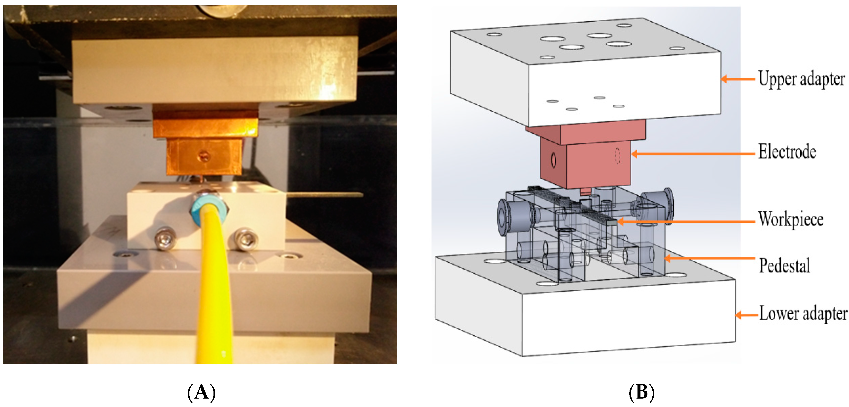
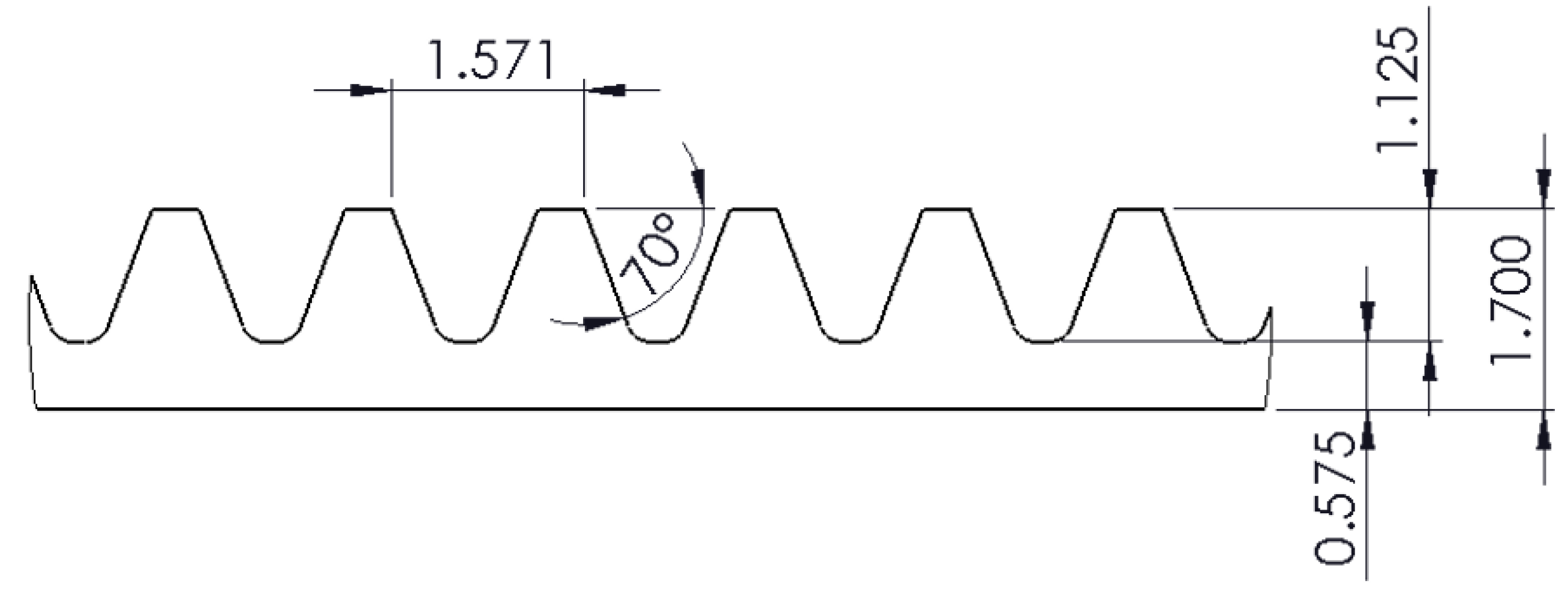
Figure 2A shows the actual device used in the experiments, Figure 2B shows the structure of the electrode module used in this study while Figure 3 shows desirable dimension of the saw tooth profile. In the experiment, the saw electrode was fixed on the upper adapter and the workpiece on the pedestal of lower adapter. The electrode was then positioned to obtain the initial gap between the workpiece and the electrode. Sequentially, the input parameters were configured on the GUI and the process was automatically started. During the processing period, the process condition was monitored using an oscilloscope.
Other basic information and settings are shown as follows: material of workpiece: SUS304 stainless steel; material of electrode: Copper Tungsten Alloy (WCU30 indicating W 70%, Cu 30%); electrolyte velocity: 10 m/sec; electrolyte temperature: 25 °C; initial gap: 100 µm; tool moving distance in the Z axis: 1200 µm; and electrolyte: 10% NaNO3.

4.2. Experimental Data

Five controllable input parameters have been chosen as experimental factors, and the range and levels of each factor are shown below. The parameters, their ranges and levels were based on the works of Satish [25] and Rajurkar et al. [26].
Voltage: (1) range: [8, 11V], (2) levels of factor: 8, 9, 10, and 11V;
Pulse on time: (1) range: [50 µs, 110 µs], (2) levels of factor: 50, 70, 90, and 110 µs;
Pulse off time: (1) range: [50 µs, 110 µs], (2) levels of factor: 50, 70, 90, and 110 µs;
Feed rate: (1) range: [5 µm/s, 8 µm/s], (2) levels of factor: 5, 6, 7, and 8 µm/s;
Electrolyte pressure: (1) range: [2.0 kg/cm2, 3.5 kg/cm2], (2) levels of factor: 2.0, 2.5, 3.0, and 3.5 kg/cm2.
In this study, two independent experiments were run with the same input parameter combination. A charge coupled device (CCD) camera was utilized to measure all the workpieces after the process of ECM saw tooth making. The experimental data is given in Appendix A.

4.3. Input-Output Modeling

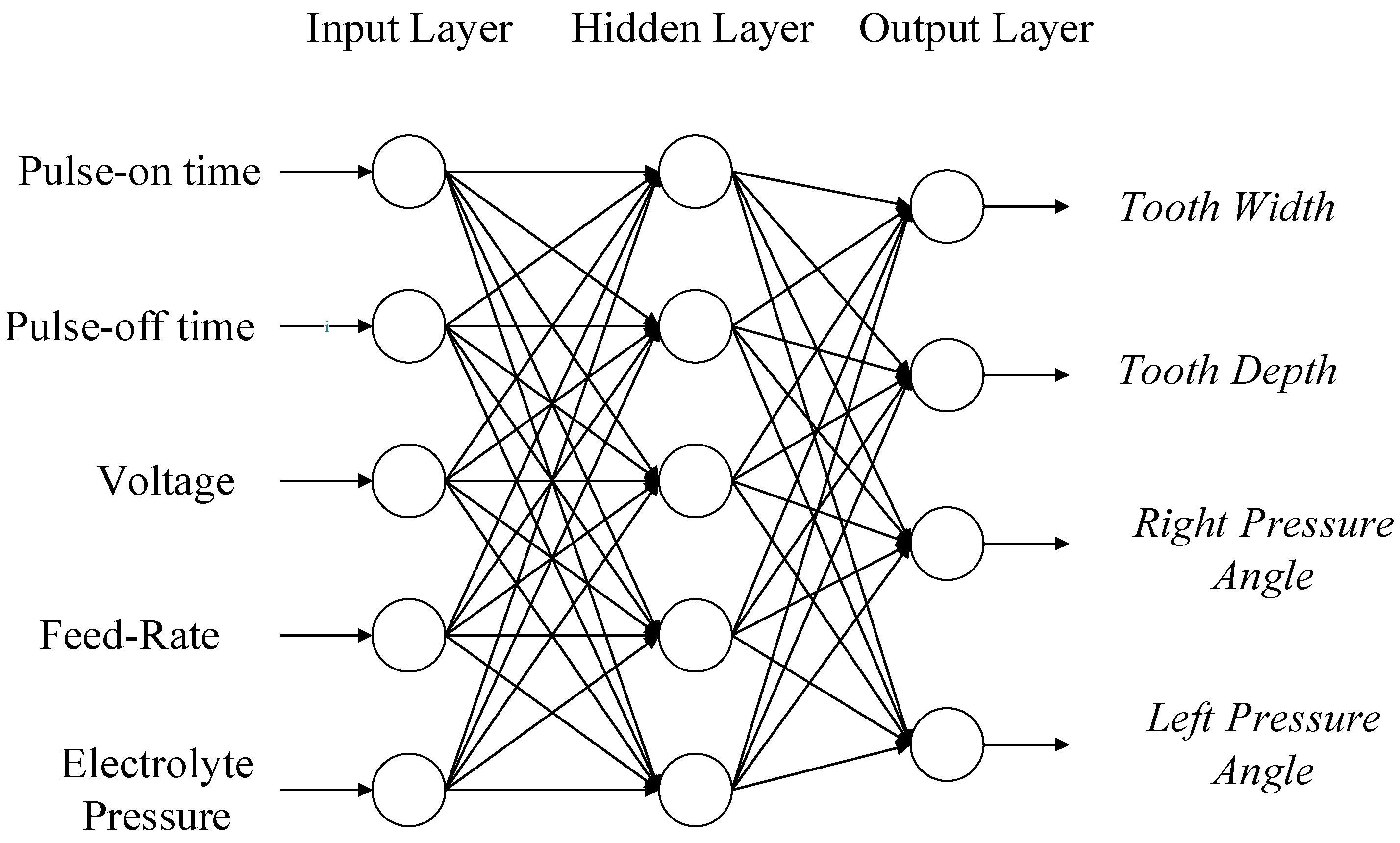
NNs are a commonly used technique for input-output mapping in many fields due to their ability to approximate functions to the desired degree of accuracy, and unlike physics-based models, the shape of the approximation function does not need to be assumed before training. Due to the lack of physics-based models, NN was used to model the relationship between the input parameters and performance indicators of the ECM. NN, as shown in Figure 4, consists of input, hidden, and output layers with weighted connections connecting the input layer to the hidden layer and the hidden layer to the output. Gradient descent (GD) and Levenberg–Marquardt (LM) are commonly used to train the weight values of the NN but as they are gradient based algorithms, their convergence to the global minimum is very sensitive to the starting points; therefore, a hybrid GA-LM algorithm was used to train the NN. GA is metaheuristic algorithm that can search the solution space more thoroughly, therefore, it was initially used to set the weights of the NN. The training of these weights was then continued with LM to leverage its rapid local convergence capabilities.
The objective of training the NN is to find a structure and a set of weight values that not only minimize the mean squared error (MSE) of the training set but is also able to predict future outputs with a high degree of accuracy. To ensure that the trained NN did not overfit to the training data, the experimental dataset was split into 3 sets: training, validation, and testing. The training set was used to train the weights of the NN, the validation set was used to ensure that the overfitting did not occur, and the testing set was used to evaluate the prediction capabilities of the trained NN structure. Once a satisfactory NN was created and trained, it was then used as the fitness function in the optimization algorithm.

4.4. Optimization Objective

In this case study, four different optimization scenarios with different single objectives were tested. In scenario 1, the optimization objective was to obtain a tooth width of 1.125 mm. The objective function for scenario 1 is shown in Equation (2).
O b j e c t i v e   1 = min | ( T o o t h w i d t h 1.125 mm ) |
In scenario 2, the optimization objective was to obtain a tooth depth of 1.194 mm. The objective function for scenario 1 is shown in Equation (3).
O b j e c t i v e   2 = min | ( T o o t h d e p t h 1.194 mm ) |
In scenario 3, the optimization objective was to obtain a left pressure angle of 20°. The objective function for scenario 1 is shown in Equation (4).
O b j e c t i v e   3 = min | ( L e f t p r e s s u r e a n g l e 20 ) |
In scenario 4, the optimization objective was to obtain a right pressure angle of 20°. The objective function for scenario 1 is shown in Equation (5).
O b j e c t i v e   4 = min | ( R i g h t p r e s s u r e a n g l e 20 ) |

5. Result and Analysis

5.1. Neural Network Model

As stated earlier, the available experimental data was divided into training, validation, and testing sets. Out of the 32 data sets available, 24 data sets were used in the training set, 4 in the validation set, and 4 in the testing set; assignments were made by random selections. During the training procedure, GA had a population size of 50, a crossover fraction of 0.8, and it was run for 500 generations. Once the training was completed using GA, the weights were then trained using the LM algorithm, which had an iteration limit of 1000. A trial-and-error method was used to determine the best NN structure, which had 5 input neurons, 1 hidden layer with 4 neurons, and an output layer with 4 neurons. To validate the trained NN, it was used to predict the outputs of the 4 different test sets and the relative error between the predicted and the actual outputs was calculated as shown in Figure 5. Table 1 shows the mean absolute percentage error for each output of all of the test sets.
As can be seen from Figure 5, the highest relative error is 7.19% for the 2nd output of the 2nd test set. All the errors are below 8% and the MAPE of the test sets are below 8%. The low values of the relative error and the MAPE indicate that the chosen NN structure was able to predict future output values with a high degree of accuracy.

5.2. Two-Stage Filter Split-Optimization

In the first stage of the proposed method, the cluster centers splitting strategy was used to obtain the k value that gave the least number of sub-search spaces. In this case study, this was obtained using a k value of 2 as indicated by Table 2. It can also be observed that if the k value was increased from 5 to 6, the number of sub-search spaces decreased, therefore, in this paper the k value was only varied from 2 to 6.
Next, the sub-search spaces, when a k value of 2 was used for each objective; the spaces were optimized to get optimal input process parameter combinations. “Best solutions” were obtained from the optimal input process parameter combinations by performing a significance check. Since the measurement error of the experimental data was ±3%, the significance level was also set as ±3%, that is, any optimal input process parameter combination whose output was within 3% of the target value would be considered a part of the “best solution” set and this set would be called solution set A. The number of solutions in solutions set A when the k value varied from 2 to 6 are shown in Table 3, Table 4, Table 5 and Table 6.
As can be observed from Table 3 (Objective 1), when the k value increased from 2 to 5, the number of sub-search spaces increased from 243 to 2592, but decreased to 1250 when a k value of 6 was used. An increase in the number of sub-search spaces meant that the optimization algorithm had a much higher probability of finding a combination of optimal input process parameters that belonged to solution set A. This hypothesis is confirmed as the number of solutions in solution set A increased from 225 to 1440 when the k value was increased from 2 to 5 but decreased to 864 when a k value of 6 was utilized. Though the number of solutions in solution set A increased significantly with an increase in k value, the efficiency of the algorithm decreased. A k value of 2 provided the highest efficiency of 92.59% while a k value of 5 provided the lowest efficiency of 55.56%. Similar trends can be observed in Table 5, Table 6 and Table 7 where the number of solutions in solution set A increased from 8 to 45, 16 to 47, and 23 to 100 when the k value increased from 2 to 5 but the efficiency decreased from 3.29% to 2.50 %, 6.58% to 2.72%, and 9.47% to 3.86% in Table 4, Table 5 and Table 6, respectively. Therefore, to find more “best solutions” at a higher efficiency, certain input process parameters were excluded from the cluster centers splitting strategy based on the standard deviation of solution set A as well as the characteristics of the experimental data. Several threshold values were tested to determine which combinations of the threshold vales would provide the highest number of “best solutions” at the highest efficiency. The test threshold values are given in Table 7.
Setting 1 requires a relatively low linear relationship between the input parameters and the optimization objective and a low standard deviation of the optimized input parameter. Settings 2 and 3, on the other hand, have a stricter linearity requirement (with setting 3 having the highest requirement), however, the standard deviation of the optimized parameters can be significantly higher. The results obtained using these settings are given in Table 8, Table 9, Table 10 and Table 11.
According to Table 8, since only input 3 (voltage) fits the requirements of both settings 2 and 3 it would be removed from the split optimization strategy for Objective 1. For Objective 2 and 3, different simulations were performed with only input 2 (pulse-on time) being removed, inputs 2 and 3 removed, and only input 3 removed. Similarly, for Objective 3, simulations were performed with inputs 1 (pulse-on time), 4 (feed rate), and 5 (electrolyte pressure) being removed, inputs 1 and 5 removed, and only input 5 removed. Lastly, for Objective 4, only input 1 was removed from the cluster centers splitting strategy.
Next, the input process parameters that were not excluded based on the results of Table 8, Table 9, Table 10 and Table 11 had their ranges split into smaller sub-ranges using the results in Table 3, Table 4, Table 5 and Table 6. In this case study, k = 5 was used for all objectives since it gave the most sub-ranges. Once the sub-search spaces had been obtained, GA was used to obtain the solution set B for each optimization objective. The sub-search spaces were then optimized using GA and solution set B was obtained for each optimization objective. Finally, solution set C was formed by combining the unique solutions from set A and set B and the efficiency was calculated using Equation (1). These results are given in Table 12.
For Objective 1, the range splitting was done after excluding pulse-off time and the total number of solutions obtained in solution set C was significantly reduced to 493 from 1440 solutions, obtained using the original method with a k value of 5 (Table 3). Noticeably, the solution efficiency increased to 90.79% compared to 55.56%, observed for the original method.
Similarly, for Objective 2, somewhat fewer solutions were obtained, while the efficiency was considerably higher using the proposed method. Additionally, the higher efficiency was achieved regardless of whether pulse-off time, voltage, or both were excluded from the cluster centers splitting strategy. The largest number of results (36) were obtained at the highest efficiency (6.63%) when pulse-off time was excluded.
For Objective 3, the highest number of solutions in solutions set C were obtained when pulse-on time was excluded from the cluster centers splitting strategy compared to when inputs pulse-on time, feed rate, and electrolyte pressure or only pulse-on time were removed. However, the highest efficiency was achieved when inputs pulse-on time, feed rate, and electrolyte pressure were removed. Again, similar trends as those for Objectives 1 and 2 were observed here, that is, higher efficiency with a slightly lower number of solutions.
Finally, for Objective 4, the proposed method provided 104 solutions when pulse-on time was removed from the cluster centers splitting strategy at 17.25% efficiency while the original method provided 106 solutions at 7.07% efficiency (Table 6, k = 4). The results from these experiments show that though the proposed method provides slightly less solutions than the original method, it can find them at a much higher efficiency than the original method.

6. Conclusions

In this paper, a two-stage filter split-optimization approach was developed to further enhance the capabilities of the split-optimization technique proposed by Rajora et al. In the proposed approach, a method was developed to investigate which input process parameters should be excluded from the original cluster centers splitting strategy with the aim of achieving a higher number of “best solutions” at a high efficiency. The proposed approach consisted of two stages: 1. an initial split-optimization stage and 2. a second split-optimization stage with certain input process parameters excluded from the cluster centers splitting strategy. An input parameter optimization problem in ECM with five controllable input process parameters was used as an application of the proposed method. Based on the results obtained from the case study the following conclusions can be made:
  • If the objective is to obtain the largest amount of “best solutions” then all process parameters should be included in the cluster centers splitting strategy and the k value that provides the largest number of sub search spaces should be used.
  • Though many “best solutions” will be obtained using the original method, they will be obtained at low efficiency.
  • To obtain multiple “best solutions” at a high efficiency, certain input process parameters should be excluded. This should be based on an analysis of the experimental data and the solutions obtained when the using a k value that provides the smallest number of sub-search spaces.
  • Some potential future work for this research is as follows:
    • Application to problems with linear and non-linear constraints. The addition of constraints on the inputs would require enhancement of the splitting strategy as it is unable to cope with constraints in its current form.
    • Application to problems with comparatively more controllable parameters. Problems with a large number of controllable parameters would give a better indicator of the proposed approach’s efficiency as significantly more sub-search spaces would be formed after the splitting strategy.
    • Utilization of other clustering algorithms (density-based spatial clustering, Gaussian mixture modelling) to split the original search space into smaller sub-search spaces and comparing their performance to the proposed approach.

Author Contributions

M.R. and P.Z.: analysis of the data, development of code and writing of the manuscript. C.-F.L., Y.-C.L., Z.F., H.C., W.C.W. and M.M.: data collection and validation. S.Y.L.: guideline for the proposed approach and comments for the paper. All authors have read and agreed to the published version of the manuscript.

Funding

The manuscript receives no external funding.

Data Availability Statement

Not applicable.

Conflicts of Interest

The authors declare no conflict of interest.

Appendix A

Table A1. Experimental data used for training and testing.
No.Pulse on Time
(µs)
Pulse off Time
(µs)
Voltage
(V)
Feed Rate
(µm/s)
Electrolyte Pressure
(kg/cm2)
Tooth Depth
(mm)
Tooth Width
(mm)
Left Pressure Angle
(°)
Right Pressure Angle
(°)
1-150508.052.01.0131.41728.43827.082
1-21.0851.45525.86625.177
2-150709.062.51.0761.44425.45524.873
2-21.0871.45125.00623.308
3-1509010.073.01.0851.40325.523.862
3-21.0991.4224.56424.483
4-15011011.083.51.0831.40323.2823.495
4-21.0851.41224.41324.071
5-170509.073.51.1371.47624.27823.282
5-21.1431.44824.17922.361
6-170708.083.01.1111.36623.33821.415
6-21.1041.35922.48321.388
7-1709011.052.51.1851.61727.56226.565
7-21.1731.61227.84526.176
8-17011010.062.01.1311.4824.65824.071
8-21.1281.49625.02224.787
9-1905010.082.51.1931.53725.9925.834
9-21.1711.56426.4124.389
10-1907011.072.01.071.4928.06826.665
10-21.0791.47428.22125.752
11-190908.063.50.9191.32224.54723.742
11-20.9011.31825.74924.261
12-1901109.053.01.0331.37527.40425.037
12-21.0181.35426.93825.926
13-11105011.063.01.0971.49728.63226.565
13-21.1051.50728.75227.195
14-11107010.053.51.1021.44727.50225.247
14-21.0611.43826.77326.112
15-1110909.082.00.9871.36628.70628.355
15-20.991.35827.29625.723
16-11101108.072.50.8581.31428.70927.691
16-20.8621.33828.20527.981

References

  1. Paraschos, P.D.; Koulinas, G.K.; Koulouriotis, D.E. Reinforcement learning for combined production-maintenance and quality control of a manufacturing system with deterioration failures. J. Manuf. Syst. 2020, 56, 470–483. [Google Scholar] [CrossRef]
  2. Hatami-Marbini, A.; Sajadi, S.M.; Malekpour, H. Optimal control and simulation for production planning of network failure-prone manufacturing systems with perishable goods. Comput. Ind. Eng. 2020, 146, 106614. [Google Scholar] [CrossRef]
  3. Dulebenets, M.A. Evaluation of non-parametric selection mechanisms in evolutionary computation: A case study for the machine scheduling problem. In Nature-Inspired Methods for Stochastic, Robust and Dynamic Optimization; IntechOpen: London, UK, 2018; pp. 23–45. [Google Scholar]
  4. Dulebenets, M.A. Archived elitism in evolutionary computation: Towards improving solution quality and population diversity. Int. J. Bio-Inspired Comput. 2020, 15, 135–146. [Google Scholar] [CrossRef]
  5. Ayvaz, S.; Alpay, K. Predictive Maintenance System for Production Lines in Manufacturing: A Machine Learning Approach Using IoT Data in Real-Time. Expert Syst. Appl. 2021, 173, 114598. [Google Scholar] [CrossRef]
  6. Ciurana, J.; Arias, G.; Ozel, T. Neural network modeling and particle swarm optimization (PSO) of process parameters in pulsed laser micromachining of hardened AISI H13 steel. Mater. Manuf. Process. 2009, 24, 358–368. [Google Scholar] [CrossRef]
  7. Mukherjee, R.; Goswami, D.; Chakraborty, S. Parametric optimization of Nd: YAG laser beam machining process using artificial bee colony algorithm. J. Ind. Eng. 2013, 2013, 570250. [Google Scholar]
  8. Teixidor, D.; Ferrer, I.; Ciurana, J.; Özel, T. Optimization of process parameters for pulsed laser milling of micro-channels on AISI H13 tool steel. Robot. Comput. Integr. Manuf. 2013, 29, 209–218. [Google Scholar] [CrossRef]
  9. Lin, H.L.; Chou, C.P. Optimization of the GTA welding process using combination of the Taguchi method and a neural-genetic approach. Mater. Manuf. Process. 2010, 25, 631–636. [Google Scholar] [CrossRef]
  10. Gowtham, K.N.; Vasudevan, M.; Maduraimuthu, V.; Jayakumar, T. Intelligent modeling combining adaptive neuro fuzzy inference system and genetic algorithm for optimizing welding process parameters. Metall. Mater. Trans. B 2011, 42, 385–392. [Google Scholar] [CrossRef]
  11. Sathiya, P.; Aravindan, S.; Haq, A.N.; Paneerselvam, K. Optimization of friction welding parameters using evolutionary computational techniques. J. Mater. Process. Technol. 2009, 209, 2576–2584. [Google Scholar] [CrossRef]
  12. Sedighi, M.; Afshari, D. Creep feed grinding optimization by an integrated GA-NN system. J. Intell. Manuf. 2010, 21, 657–663. [Google Scholar] [CrossRef]
  13. Rao, R.V.; Pawar, P.J. Grinding process parameter optimization using non-traditional optimization algorithms. Proc. Inst. Mech. Eng. Part B J. Eng. Manuf. 2010, 224, 887–898. [Google Scholar] [CrossRef]
  14. Rajora, M.; Zou, P.; Yang, Y.G.; Fan, Z.W.; Chen, H.Y.; Wu, W.C.; Li, B.; Liang, S.Y. A split-optimization approach for obtaining multiple solutions in single-objective process parameter optimization. SpringerPlus 2016, 5, 1424. [Google Scholar] [CrossRef] [Green Version]
  15. Rao, R.V.; Pawar, P.J.; Shankar, R. Multi-objective optimization of electrochemical machining process parameters using a particle swarm optimization algorithm. Proc. Inst. Mech. Eng. Part B J. Eng. Manuf. 2008, 222, 949–958. [Google Scholar] [CrossRef]
  16. Jain, N.K.; Jain, V.K. Optimization of electro-chemical machining process parameters using genetic algorithms. Mach. Sci. Technol. 2007, 11, 235–258. [Google Scholar] [CrossRef]
  17. Chakradhar, D.; Gopal, A.V. Multi-objective optimization of electrochemical machining of EN31 steel by grey relational analysis. Int. J. Modeling Optim. 2011, 1, 113. [Google Scholar] [CrossRef]
  18. Senthilkumar, C.; Ganesan, G.; Karthikeyan, R. Parametric optimization of electrochemical machining of Al/15% SiC p composites using NSGA-II. Trans. Nonferrous Met. Soc. China 2011, 21, 2294–2300. [Google Scholar] [CrossRef]
  19. Rao, R.V.; Kalyankar, V.D. Parameters Optimization of Advanced Machining Processes Using TLBO Algorithm; EPPM: Singapore, 2011; pp. 21–31. [Google Scholar]
  20. Santhi, M.; Ravikumar, R.; Jeyapaul, R. Optimization of process parameters in electro chemical machining (ECM) using DFA-fuzzy set theory-TOPSIS for titanium alloy. Multidiscip. Modeling Mater. Struct. 2013, 9, 243–255. [Google Scholar] [CrossRef]
  21. Samanta, S.; Chakraborty, S. Parametric optimization of some non-traditional machining processes using artificial bee colony algorithm. Eng. Appl. Artif. Intell. 2011, 24, 946–957. [Google Scholar] [CrossRef]
  22. Goswami, R.; Chaturvedi, V.; Chouhan, R. Optimization of electrochemical machining process parameters using Taguchi approach. Int. J. Eng. Sci. Technol. 2013, 5, 999. [Google Scholar]
  23. Hartigan, J.A.; Wong, M.A. Algorithm AS 136: A k-means clustering algorithm. J. R. Stat. Soc. 1979, 28, 100–108. [Google Scholar] [CrossRef]
  24. Asokan, P.; Kumar, R.R.; Jeyapaul, R.; Santhi, M. Development of multi-objective optimization models for electrochemical machining process. Int. J. Adv. Manuf. Technol. 2008, 39, 55–63. [Google Scholar] [CrossRef]
  25. Sathish, T. Experimental investigation of machined hole and optimization of machining parameters using electrochemical machining. J. Mater. Res. Technol. 2019, 8, 4354–4363. [Google Scholar] [CrossRef]
  26. Rajurkar, K.P.; Sundaram, M.M.; Malshe, A.P. Review of electrochemical and electrodischarge machining. Procedia Cirp 2013, 6, 13–26. [Google Scholar] [CrossRef] [Green Version]
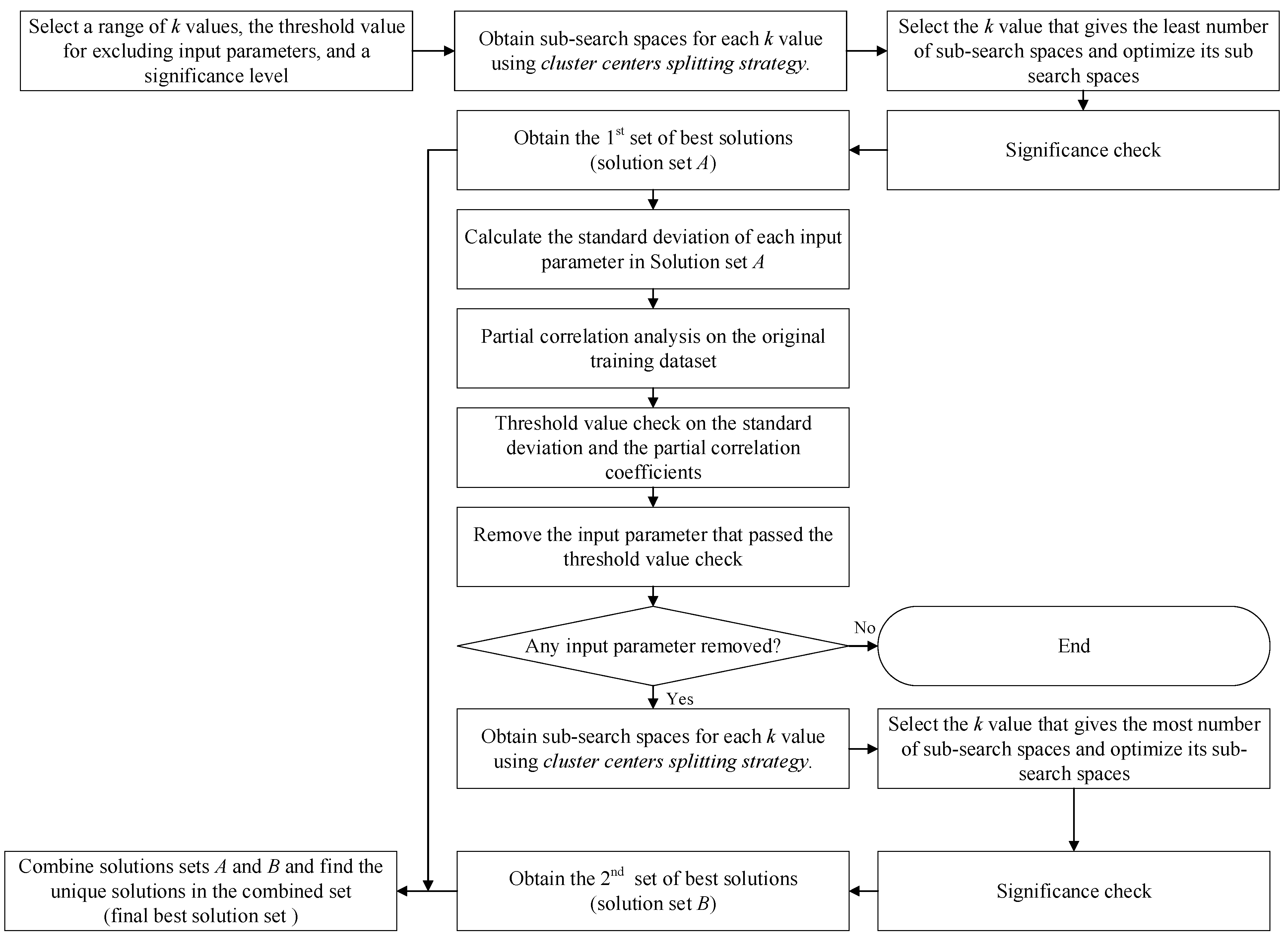
Figure 1. Flow chart of the two-stage filter split-optimization approach.
Machines 09 00065 g001
Figure 2. The structure of the electrode module: (A) actual device used during experimentation and (B) 3D design of the electrode module.
Machines 09 00065 g002
Figure 3. The desirable dimensions of the saw tooth profile (m = 0.5). All dimensions are in millimeters (mm).
Machines 09 00065 g003
Figure 4. Neural network structure used for prediction of outputs.
Machines 09 00065 g004
Figure 5. Relative error between predicted and actual output for test sets.
Machines 09 00065 g005
Table 1. Mean absolute percentage error (MAPE) for the test sets.
Test Set 1 (%)Test Set 2 (%)Test Set 3 (%)Test Set 4 (%)
MAPE1.693.382.372.18
Table 2. Number of sub-search spaces obtained for each objective under different k values.
Objectivek-Value
23456
1243576120025921250
2243576120018001200
3243576100017281500
4243768150025921000
Table 3. Number of solutions in solution set A and the efficiency of the original method obtained using the original method for Objective 1.
k-ValueNumber of Solutions in Solution Set ANumber of Searched Sub-SpacesEfficiency (%)
222524392.59
345557678.99
4839120069.92
51440259255.56
6864125069.12
Table 4. Number of solutions in solution set A and the efficiency of the original method obtained using the original method for Objective 2.
k-ValueNumber of Solutions in Solution Set ANumber of Searched Sub-SpacesEfficiency (%)
282433.29
3165762.78
42012001.67
54518002.50
62212001.83
Table 5. Number of solutions in solution set A and the efficiency of the original method obtained using the original method for Objective 3.
k-ValueNumber of Solutions in Solution Set ANumber of Searched Sub-SpacesEfficiency (%)
2162436.58
3295765.03
45110005.10
54717282.72
65115003.40
Table 6. Number of solutions in solution set A and the efficiency of the original method obtained using the original method for Objective 4.
k-ValueNumber of Solutions in Solution Set ANumber of Searched Sub-SpacesEfficiency (%)
2232439.47
3547687.03
410615007.07
510025923.86
65410005.40
Table 7. Settings of threshold for removing input process parameters.
Settings #Absolute Value of r Valuep ValueStandard Deviation
1≥0.50≤0.01≤0.15
2≥0.60≤0.01≤0.30
3≥0.70≤0.01≤0.45
Table 8. Input process parameters excluded from cluster centers splitting strategy for Objective 1.
Absolute Value of Partial Correlation Coefficient
(r Value)
Standard DeviationRemoved
Pulse on Time0.560.32No
Pulse off Time0.590.22No
Voltage0.710.22Yes (based on settings 2 and 3)
Feed Rate0.010.31No
Electrolyte Pressure0.030.25No
Table 9. Input process parameters excluded from cluster centers splitting strategy for Objective 2.
Absolute Value of Partial Correlation
Coefficient (r Value)
Standard DeviationRemoved
Pulse on Time0.290.51No
Pulse off Time0.630.12Yes (based on settings 1 and 2)
Voltage0.820.22Yes (based on settings 2 and 3)
Feed Rate0.400.15No
Electrolyte Pressure0.460.25No
Table 10. Input process parameters excluded from cluster centers splitting strategy for Objective 3.
Absolute Value of Partial Correlation
Coefficient (r Value)
Standard DeviationRemoved
Pulse on Time0.760.11Yes (based on settings 1, 2, and 3)
Pulse off Time0.100.13No
Voltage0.350.12No
Feed Rate0.550.00Yes (based on settings 1)
Electrolyte Pressure0.620.13Yes (based on settings 1 and 2)
Table 11. Input process parameters excluded from cluster centers splitting strategy for Objective 4.
Absolute Value of Partial Correlation
Coefficient (r Value)
Standard DeviationRemoved
Pulse on Time0.660.15Yes (based on settings 2)
Pulse off Time0.150.21No
Voltage0.290.18No
Feed Rate0.410.11No
Electrolyte Pressure0.590.16No
Table 12. Number of solutions in solution set C and the efficiency of the original method obtained after excluding input process parameters for all the four objectives.
ObjectiveInputs RemovedNumber of Solutions in Solution Set CTotal Number of Searched Sub-SpacesEfficiency (%)
1449354390.79
22365436.63
2 and 3152935.12
3255134.87
31, 4, and 5232638.75
1 and 5253187.86
1476187.61
4110460317.25
Publisher’s Note: MDPI stays neutral with regard to jurisdictional claims in published maps and institutional affiliations.