
An Improved Invariant Kalman Filter for Lie Groups Attitude Dynamics with Heavy-Tailed Process Noise


1
Key Laboratory of Advanced Process Control for Light Industry, Institute of Automation, Jiangnan University, Wuxi 214111, China
2
School of Electronics and Information Engineering, Harbin Institute of Technology, Shenzhen 518055, China
3
Department of Electronic and Computer Engineering, Hong Kong University of Science and Technology, Hong Kong, China
*
Author to whom correspondence should be addressed.
Machines 2021, 9(9), 182; https://doi.org/10.3390/machines9090182
Submission received: 20 July 2021
/
Revised: 21 August 2021
/
Accepted: 23 August 2021
/
Published: 27 August 2021
(This article belongs to the Special Issue Modeling, Sensor Fusion and Control Techniques in Applied Robotics)
Abstract
:Attitude estimation is a basic task for most spacecraft missions in aerospace engineering and many Kalman type attitude estimators have been applied to the guidance and navigation of spacecraft systems. By building the attitude dynamics on matrix Lie groups, the invariant Kalman filter (IKF) was developed according to the invariance properties of symmetry groups. However, the Gaussian noise assumption of Kalman theory may be violated when a spacecraft maneuvers severely and the process noise might be heavy-tailed, which is prone to degrade IKF’s performance for attitude estimation. To address the attitude estimation problem with heavy-tailed process noise, this paper proposes a hierarchical Gaussian state-space model for invariant Kalman filtering: The probability density function of state prediction is defined based on student’s t distribution, while the conjugate prior distributions of the scale matrix and degrees of freedom (dofs) parameter are respectively formulated as the inverse Wishart and Gamma distribution. For the constructed hierarchical Gaussian attitude estimation state-space model, the Lie groups rotation matrix of spacecraft attitude is inferred together with the scale matrix and dof parameter using the variational Bayesian iteration. Numerical simulation results illustrate that the proposed approach can significantly improve the filtering robustness of invariant Kalman filter for Lie groups spacecraft attitude estimation problems with heavy-tailed process uncertainty.
1. Introduction
The navigation and control operations in aerospace engineering usually require adequate accurate knowledge of spacecraft orientation in space, and attitude determination from vector observations is usually employed in astronautically applications [1,2,3,4]. The widely used Kalman type filters can infer the state in Euclidean vector space by fusing attitude dynamic and observation sensor according to their probabilities [5,6,7,8]. Recently, the building of attitude dynamics on matrix Lie groups has been investigated actively for the navigation and control of spacecraft targets because it can significantly improve the estimation and control performance to make full use of the geometrical properties of Lie groups models [9,10].
For attitude estimation, there have already been significant research interests in the estimation and control of spacecraft targets such as the invariant observers and filters for attitude dynamics on the special orthogonal group SO(3), or the navigation systems defined on the special Euclidean group SE(3) [11,12]. Accounting for the geometrical invariance of symmetry attitude dynamics, the resulted attitude description with rotation matrix on SO(3) can avoid the trouble of singularities and unwinding encountered when using unit quaternion [13] and, to some extent, also contribute to better estimation performance for attitude determination algorithms [14]. Exploiting the mapping relation between matrix Lie groups and Lie algebra, invariant Kalman filter (IKF) can convert the attitude dynamics on SO(3) to Euclidean vector space and mimic classical Kalman filtering steps [15]. IKF is based on the invariance and log-linearity of symmetry dynamics, which then leads to better convergence on a much bigger set of state trajectories [16]. In these available researches, the process noise of attitude dynamical model was assumed to be a concentrated Gaussian distribution [17,18] and the statistics parameter are also assumed to be accurately given in advance as required in classical Kalman theory [19,20]. However, due to the presence of server maneuvers in space missions, there might be some unpredictable disturbances or outliers that would contaminate the Gaussian distribution and violate the required assumptions for Kalman filtering on matrix Lie groups.
For Euclidean space filtering problems, some adaptive methods are commonly used to deal with the trouble of inaccurate/unknown noise parameters [21,22,23]. Some adaptive techniques have been designed to estimate online unknown/inaccurate noise parameters, mainly including innovation-based adaptive methods and multiple model methods [24,25,26]; nevertheless, the convergence of innovation-based estimation methods cannot be guaranteed while the parallel-running multiple filter banks might increase the computational complexities. The variational Bayesian(VB) iteration-based adaptive methods have also been employed to jointly determine the system state and inaccurate noise statistics [27,28,29]. However, these adaptive methods all assume the noise distribution to be Gaussian and cannot be applied to the filtering cases with heavy-tailed noise. For heavy-tailed system noises, the Student’s t distribution assumes the distribution of the latent state and system noises as a joint Student’s t-distribution, and it has been proved to be more suitable to represent the non-Gaussian probability density function (PDF) [30,31].
To deal with the heavy-tailed process noise caused by severe maneuvering of rigid bodies, a robust Student’s t-based hierarchical Gaussian system model for the SINS/GPS integration is presented by modeling the prior probability density function as a Student’s t distribution and the conjugate prior distributions [21]. To improve the filtering performance of Student’s t-based methods for cases with both heavy-tailed process and observation noises, a robust Student’s t-based Kalman filter is proposed employing the variational Bayesian-based iterative approach in [32]; in the work of [33], by applying the Student’s t approximate distributions to posterior filtering and smoothing probability density functions, the robust nonlinear Student’s t-based filter and smoother are also presented as the generalization and extension of the linear Student’s t filtering methods. Note that the above researches provide a sound theoretical foundation for attitude estimation problems with heavy-tailed noises, but they are originally designed in Euclidean space systems for filtering of vector variable states. To the best of our knowledge, for attitude estimation problem in SO(3), until now there is still no special study on the robust Student’s t-based adaptive methods for invariant Kalman filtering on matrix Lie groups.
Note that although the available invariant Kalman filter also obeys the basic theory of classical Kalman filter, the above researches about robust Student’s t-based methods cannot be directly applied to matrix Lie groups systems. The uncertainty definition of concentrated Gaussian distribution on matrix Lie groups requires the assumption of noisy errors being small enough [34,35], which is the condition for first order approximation to the Baker–Campbell–Hausdorff (BCH) formula [36,37]. For attitude estimation on SO(3) in aerospace engineering, the presence of heavy-tailed noises and disturbances imposes a critical constraint on the application of robust Student’s t-based methods to improve the performance of invariant Kalman filter.
According to the above discussions, it is rather meaningful to investigate the robust Student’s t-based invariant Kalman filtering method especially for the matrix Lie groups attitude estimation problems in the presence of heavy-tailed outliers in system process noise. In this work, for attitude estimation problem with heavy-tailed process noise, this paper proposes a hierarchical Gaussian state-space model for invariant Kalman filtering, and the Lie groups rotation matrix of spacecraft attitude is inferred together with the scale matrix and dof parameter using the variational Bayesian iteration. Numerical simulation results illustrate that the proposed approach can significantly improve the filtering robustness of invariant Kalman filter for Lie groups spacecraft attitude estimation problems with heavy-tailed process uncertainty.
2. Primaries and Problem Definition
2.1. The Attitude Estimation System on the Special Orthogonal Group SO(3)
Attitude determinition from two vector observations is an important task in most aerospace engineering. The attitude dynamic on special orthogonal group with the associated observation vectors can be formulated as the following system model [1,14]
where the special orthogonal group is the group of 3 × 3 rotation matrices and is the mapping rotation from the body frame of the spacecraft to the earth-fixed frame at time instant ; denotes the control rotation; is a composition of the vector observations with their respective observation vector ;, and are Gaussian white and mutually independent observation noises with denoting the Gaussian distribution. Note that the vector observation based attitude determination is a common application scenario because the Sun sensor, magnetometer, horizon sensor, and the gravitational accelerometer are usually equipped by most spacecrafts in astronautical engineering [1]. A graphical presentation of target application scenario is given in Figure 1.
Note that the additive forms of vector noises in Euclidean space are not supported in Lie Groups space. The vector process noise is injected through Lie exponential operator and, for any , the projection between the vector noise and the associated groups element are
where is the matrix exponential operator and is the skew-symmetric matrix. The concept of concentrated Gaussian distribution (CGD) was employed to define the probability distribution for random variables on matrix Lie groups [19,20,37]. For attitude estimation, in concentrated Gaussian distribution the groups variable with mean and covariance is defined as
where denotes the concentrated Gaussian distribution (CGD). Note that, in the definition of CGD, the eigenvalues of are assumed to be small enough, i.e., almost all the mass of the distribution should be concentrated in a small neighborhood around the mean of the rotation variable [20,37]. A graphical illustration of the relation between the concentrated Gaussian distribution on matrix Lie groups SO(3) and the classical Gaussian distribution relation is presented in Figure 2.
2.2. Model Projection Based on the Invariance Property of Attitude Estimation System
For attitude estimation on SO(3), the usual Kalman filtering methods in Euclidean vector space could not be applied directly. However, by properly defining the system variable, the Lie groups dynamic model (1) can be projected into the usual Euclidean space based on the invariance property. Let be an estimate for at instant k − 1 and be the prediction for . Define the invariant error , then the evolution model of invariant error obeys
where the of the last step is a first order form of the Baker–Campbell–Hausdorff (BCH) formula [34,35,36]. Note that if the norm of the error term and are small enough so that the second order term in (7) could be negligible, then the matrix Lie groups attitude dynamic (1) for rotation matrix could be approximately converted into the following linear state space model in Euclidean space for the invariant error
As for observation model (2), the observation sequence can also be reformulated into a function of the invariant error , i.e., the new innovation sequence [14]
where and are the projected observation matrix and noise, respectively; note that, since the observation noises are isotropic and mutually independent noises and with , we have .
Obviously, based on the definition of the invariant error , the Lie groups dynamics (1) and observation model (2) could be converted as the Euclidean space model (8) and (9) for the invariant error (as in Figure 3). Note that both the true rotation state and the control rotation do not appear in the converted model (8) and (9); therefore, the evolving motion of is actually independent of the true trajectory of rotation and control rotation , which is called the invariance property of symmetry model [15,16].
2.3. The Invariant Kalman Filter for Attitude Estimation
As the consequence of invariance property, for the attitude estimation system, the probability distribution of rotation state based on the observation is equivalent to that of the invariant error in , constituting the basis of invariant Kalman filter. Then, if the process noise obeys classical Gaussian distribution, i.e., , the filtering steps for attitude estimation system on Lie group SO(3) can be implemented by mimicking that of the classical Kalman filter for invariant error in Euclidean space.
For the attitude dynamic (1) and associated observation (2), invariant Kalman filter (IKF) aims to recursively predict and correct the estimate for the rotation state. Given the initial estimate for true with error , as the prediction for prior error estimate based on (8), the prior error rotation estimate based on the dynamic model (1) can be implemented as follows
where and are the prior and posterior error estimate for true rotation state , respectively; and are associated with the prior and posterior error estimate for true error . The covariance propagation of rotation group is same as that of the classical Kalman filter for invariant error based on the evolution model (8),
where stands for the covariance of the posterior estimate and . Therefore, based on the converted innovation (9), the correction steps of IKF for the rotation state can be implemented by updating the estimate with innovation sequence
where is the Kalman gain matrix, and the posterior estimate is then updated with Lie exponential operation of the correction term as in (12) [16,17]. A graphical presentation of the filtering diagram of invariant Kalman filter is presented in Figure 4.
2.4. The Attitude Estimation Problem with the Trouble of Heavy-Tailed Process Noise
Obviously, the invariant Kalman filter (IKF) is a general extension of the Euclidean space Kalman filter to matrix Lie groups systems based on the invariance property of symmetry dynamics [16]. However, for the attitude estimation in aerospace engineering, there is still some difficulty for practical implementation of the IKF-based attitude estimation because the presence of heavy-tailed process noise in attitude dynamic might introduce great challenge and trouble to the theory of IKF:
Firstly, in the filtering step (10)~(14) of IKF, the process noise of attitude was assumed to be a concentrated Gaussian distribution and the statistics parameter is also required to be accurately known (as in Figure 4). However, due to the presence of severely maneuvering operations in space tasks, there might be some unpredictable disturbances or substantial outliers that would contaminate the Gaussian distribution and violate the assumptions for Kalman filtering on matrix Lie groups. Therefore, the theoretical foundation for optimal Kalman filtering is sure to be destroyed, which will degrade the final estimation.
Secondly, for the invariant projection of the Lie groups dynamics (1) into the linear vector form (8) in Section 2.2, the first order approximation to BCH formula is employed based on the assumption that both and were small enough and the second and higher order residual could be dropped from (7) to (8). However, for aerospace engineering applications, the unpredictable disturbances or substantial outliers caused by severely maneuvering operations might violate this condition and lead to inaccurate approximation to the system model, which is prone to a potential source of error and influences the estimation accuracy of IKF.
For attitude determination in astronautical engineering, it is rather meaningful to further study Lie groups estimation problems with heavy-tailed process noise and investigate new robust adaptive version of invariant Kalman filtering methods to improve the filtering precisions for cases with heavy-tailed process noises.
3. Robust Student’s t Based Invariant Kalman Filter for Attitude Estimation on SO(3)
3.1. Probability View of Attitude Estimation with Heavy-Tailed Process Noise
For attitude estimation, if the process noise in dynamic model (1) is heavy-tailed and contaminated by larger outliers, the Gaussian distribution and concentrated Gaussian distribution cannot accurately describe the probability distribution of heavy-tailed process noise. In this work, to account for the larger outliers due to severely maneuvering, the probability of the heavy-tailed noise is described as the student’s t distribution
where denotes the probability density of the process noise ; denotes the student’s t distribution with mean vector , scale matrix , and degree of parameter ; is an auxiliary random variable in (15); and represents the Gamma probability density function of the scalar with and as the shape and rate parameter, i.e.,
where is the natural constant and represents the Gamma function. Obviously, the probability density function of the student’s t distribution can be regarded as the infinite mixture of the classical Gaussian probability density function [21,30].
If given the Gaussian approximation of the posterior probability density function and concentrated Gaussian approximation of posterior for instant k−1, the prior probability density function of and for time instant k can be obtained according to the Chapman–Kolmogorov equation [38,39],
where denotes the posterior probability density function of the based on the innovation sequence from time instant 1 to k − 1 and denotes the posterior probability density function of rotation based on observation from instant 1 to k − 1. Note that resorting to the equivalence of the and in probability density function, is the student’s t distribution for system process noise and so we have . Further, it is evident that the prior probability for instant k is not Gaussian but a student’s t distribution with mean vector parameter , scale matrix and parameter , i.e.,
where , , and are the mean vector, scale matrix, and degree of freedom parameter of the prior student’s t distribution ; and is the auxiliary random variable. Employing (15)~(19), the prior student’s t distribution can be reformulated into a hierarchical composition of the Gaussian distributions
Attitude estimation aims to propagate the posterior probability density distribution based on the observation . Since the observation noise in (2) and its equivalent form in (9) are zero mean Gaussian white sequence with covariance , the likelihood probability density function of the innovation sequence based on the error is equal to that of observation given the rotation , i.e.,
where is the probability density function of given rotation , and is the probability density function of based on error .
Note that the accurate propagation of the probability density function requires accurate knowledge of scale matrix and degree of freedom . However, for real engineering applications in the presence of unpredictable disturbances or substantial outliers, these two distribution parameters are usually not correct or unavailable in advance. Therefore, from the view of probability density, the main troubles of attitude estimation with heavy-tailed process noise are threefold:
- (1)
- With the student’s t distribution process noise, the probability density function in classical invariant Kalman filter depends on the auxiliary random variable and becomes the hierarchical form in (20) and (21).
- (2)
- For the unpredictable disturbances or outliers induced by severely maneuvering operations, the accurate scale matrix and degree of freedom are usually unavailable but essential to propagate the posterior estimates.
As a consequence, the heavy-tailed attitude estimation problem cannot be solved with the invariant Kalman filter in Section 2 since the distribution parameter and should be estimated together with the invariant error and the rotation state .
3.2. Prior Probability Definition for the Parameters of Student’s t Distribution
To solve Lie groups filtering problems with Student’s t distribution process noise, this work aims to estimate the rotation group state together with and by variational Bayesian iterations as in Figure 5. The prior distributions of parameter and based on all historical observation sequences should be conjugate prior distributions so that their posterior distribution would maintain the same form as their prior distribution.
According to (20) and (21), the estimated scale matrix is proportional to the covariance matrix of Gaussian distribution. Therefore, the commonly used inverse Wishart distribution and the Gamma distribution of Bayesian statistics are employed as the conjugate prior distributions for parameters and , respectively.
The distribution of scale matrix is defined as inverse Winshart distribution [29,39,40] which is often used as conjugate prior for the covariance matrix of the Gaussian variable. For attitude estimation problem, the inverse Winshart function of can be written as
where denotes the inverse Winshart distribution; denotes the degrees of freedom; is the inverse scale matrix; is the determinant operator; and is the 3-variate gamma function [29]. For the scale matrix , the expectation of the matrix inverse is and so we have
The distribution parameter can be defined as the Gamma distribution [21],
where are respectively the shape and rate parameter of the Gamma distribution , respectively.
In summary, Equations (20)~(25) actually constitute a new student’s t-based hierarchical Gaussian state-space model for the heavy-tailed attitude estimation problem, whose diagram is presented in Figure 6. The initialization of the required distribution parameter is based on the nominal parameter , which will be discussed later on. Using the above distribution definition, the rotation state and , the auxiliary random variable , the scale matrix , and the parameter will be jointly estimated based on the newly constructed hierarchical Gaussian state-space model by variational Bayesian iterations, which then leads to the new robust student’s t-based invariant Kalman filter for the heavy-tailed attitude estimation problem.
3.3. Variational Beayesian Approximations of Posterior Probability Density Function
To jointly estimate the rotation state , auxiliary random variable , scale matrix , and parameter requires calculating the posterior probability density function . Since the accurate analytical expression of is not available, this work tries to obtain its factored approximate based on variational Bayesian iterations [38]. i.e.,
where , , , and represent, respectively, the approximate posterior probability density function of , , , ; , , and , which can be determined by minimizing the Kullback–Leibler divergence (KLD) [38,41] between the factored approximate and the true [29,38], i.e.,
where denotes the KLD between and . According to the variational Bayesian iteration, these approximate posterior , , , and to (27) satisfy the following equations [21,38]
where denotes the natural logarithm function; represents the mathematical expectation operation for all variables except , while , , and are with similar definitions; is the constant with respect to , while , , and are similarly defined. Obviously, Equations (28)~(31) are coupled and so no analytical solutions to the above equations exist. Therefore, only the approximate solutions are available and in this work the fixed-point iterations are employed to determine these parameters [38].
According to the conditional independence properties, the joint probability density function can be factored as follows
Then, using (20)~(26), we have
Using (16) and (24), can be formulated as
3.4. Fixed-Point Iteration of the System State and Distribution Parameters
Based on the conditional independence property of the invariant error and parameters , , and , the Equations (28)~(31) can be rewritten with above Equation (34) and fixed-point methods can be used to obtain the approximate estimates to the invariant error as well as the parameters ,, and [21].
3.4.1. Fixed-Point Iteration of the Invariant Error
With (34) and the independence property of and , (28) can be written as
where is the iterative approximation to at i + 1th iteration; represents the mathematical expectation at ith iteration for variables except the invariant error while and denote the mathematical expectation at ith iteration for and , respectively; is the modified prior error covariance matrix calculated as
Then, can also be updated as a Gaussian distribution, i.e.,
where and can be determined by following the update steps
where denotes the calibrated Kalman gain matrix at the i + 1th iteration.
3.4.2. Fixed-Point Iteration of the Auxiliary Random Variable
Using (34) and conditional independency, the in (29) can be rewritten as
where represents the mathematical expectation at ith iteration for variables except the while denotes the mathematical expectation at ith iteration for the parameter . Note that the approximate and updated in (35)~(40) can be used to propagate Equation (41) and the term can be reformulated as
Then (41) could be deduced into
which is actually also a Gamma distribution as (16), i.e.,
where and are the shape and rate parameter determined by
3.4.3. Fixed-Point Iteration of the Prior Estimate for Covariance Matrix
With (34), (37), (44) and the independence of and , (30) can be rewritten as
where the term is calculated as
Therefore, using (24) and (47), is also an inverse Wishart distribution as
where are given as
3.4.4. Fixed-Point Iteration of the Prior Estimate for Parameter
With (34), (37), (44), and (49), (33) can be rewritten as
With Stirling’s equation , (52) can be approximated as
Therefore, using (16) and (53), can be updated as a Gamma distribution, i.e.,
where are given as
3.5. The Variational Beayesian Iteration Based Robust Student’s t Invariant Kalman Filter
To propagate the approximate posterior distributions, using (44), (49) and (54), the expectations , , , and can be calculated as follows
where represents a digamma function [42]. After N times of fixed-point iterations, the required posterior probability density function of could be approximated as
where are respectively the posterior estimate for invariant error and the posterior estimate error covariance parameter. Then, resorting to the equivalence of probability distribution, the distributing of the propagated rotation state can be updated as the concentrated Gaussian distribution with mean being and covariance being ,i.e.,
where the iterative Kalman gain matrix is calculated in (39). The Equations (62) and (63) are actually the projection of the Euclidean space Equation (38) into Lie group space.
Therefore, the filtering steps of the proposed approach include the steps (36)~(40), (42)~(46), (48)~(51), and (54)~(63). The detailed implementation of the proposed method for attitude estimation is presented in Algorithm 1. For the heavy-tailed attitude estimation, the nominal could be selected as (11) to initialize the filter parameter and ; the invariant error is defined as the Lie exponential error of and so it could be assumed to be zero at the initialization to propagate the prior estimate .
In invariant Kalman filter, the prior error estimate is actually based on all the historical observations before time instant k. In this work, the covariance parameter is also inferred using the historical observations until time instant k. As for the inverse Wishart distribution of , at time instant k the degree of parameter is set as and the inverse scale matrix parameter is set as .
In practical numerical integration of the attitude dynamic model, if there exists severe maneuvering, the system process noise will have a heavy-tailed distribution and the degree of freedom parameter depends on the maneuvering intensity. According to our experience, the initial estimates for the shape parameter and rate parameter could be set as for the iteratively updating in Algorithm 1.
| Algorithm 1. The filtering steps of one time instant in the proposed approach for attitude estimation. |
| Inputs:,,,,,,,, 1. Predict the nominal invariant error and rotation according to (8) and (10) , 2. Predict the nominal prior error covariance according to (11) 3. Calculate the converted innovation according to (9) 4. Initialize the prior parameters ,, 5. Calculate initial expectations according to (24) and (25) , for i = 0:N − 1 6. Update according to (36)~(40) ,, , 7. Update according to (44)~(46) , 8. Update according to (48)~(51) ,, 9. Update expectations , and according to (57)~(59) ,, 10. Update according to (55) and (56) , 11. Calculate the expectation according to (60) end for 12. Update the posterior rotation group and its covariance according to (63) , |
| Outputs: , |
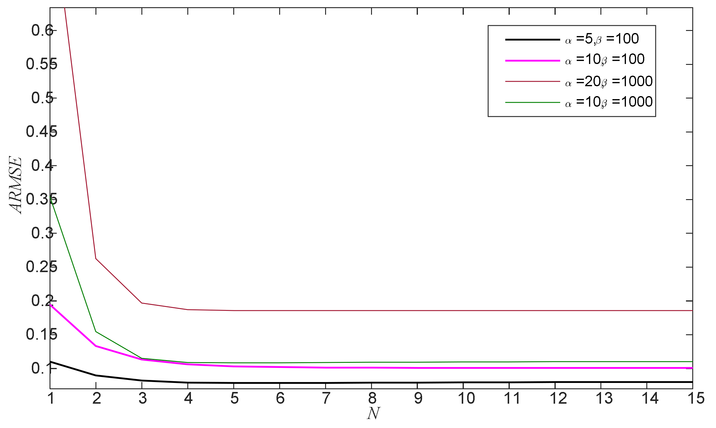
The number of N iterations is also a crucial parameter for proposed approach and, generally, it should be set to a value larger than the system dimension to guarantee the local convergence of variational Bayesian iterations; nevertheless, a too larger value is sure to increase the computational cost for algorithm implementation. The balance between precision and cost should be considered according to the detailed applications.
4. Numerical Simulations
To further demonstrate the performance of the variational Bayesian iteration-based invariant Kaman filter, the attitude estimation system (6) (7) is simulated with parameter The real attitude trajectories are generated for 5000 s and the heavy tailed process noise is generated with heavy tailed outliers according to [42], i.e.,
which means that percentage of process noise is drawn from a Gaussian distribution with covariance while the covariance of percentage of process noise is severely increased by scale parameter due to the presence of outliers.
As a comparison, the filtering methods of the proposed approach (RSIKF), IKF [14,16] the Student’s t filter (STF) [43], the Huber-based Kalman filter (HKF) [44], and the QeIKF [24,25] are conducted together. For HKF, the tuning parameter is set to 1.345 and the number of iterations is selected as 10; in STF the degree of freedom parameter is selected as 3. In the proposed RSIKF, the filter parameters are set to , , , . All above filtering methods are implemented with MATLAB codes on a computer with Intel Core i7-7700 CPU at 3.60 GHz. To compare their performance, the error variable in Lie algebra of 5000 random runs is used to calculate the root mean square error during the 5000 runs’ filtering time and average root mean square error , i.e.,
where denotes the true estimate at the k-th time instant of the l-th simulation run and is the corresponding estimate for the true ; denotes the Euclidean vector norm.
In this work, three cases of heavy tailed process noises are simulated with = 5, 20 and = 100, 1000 to investigate the filtering performance of different methods. The ARMSE result data of different filtering methods are given in Figure 7 while the result data during the first 500 runs’ filtering processes are presented in Figure 8 and Figure 9.
The ARMSE result of IKF in Figure 7 and data of IKF in Figure 8, Figure 9, Figure 10 and Figure 11 are always the largest in all methods for all cases, which certifies that the estimation performance of IKF is severely corrupted by heavy tailed outliers.
In STF, the noise distribution is assumed as a given Student’s t distribution, and the ARMSE result in Figure 7 and in Figure 8, Figure 9, Figure 10 and Figure 11 is smaller than that of IKF. However, since it still requires accurate prior knowledge of the noise distribution parameter, the unknown or inaccurate parameters still mislead the estimate results.
The QeIKF aims to estimate, online, the unknown noise covariance parameter and also output better results than IKF and STF; however, it assumes the distribution as an Gaussian one so its ARMSE result in Figure 7 and in Figure 8 for the case = 5 become worse than the case of = 20 in Figure 9; while, as shown in Figure 10 and Figure 11, its filtering precision would be significantly degraded by large outliers with = 1000.
HKF shows some robustness to heavy tailed outliers IKF, STK, and QeKF for the cases of = 1000 as in Figure 10 and Figure 11. Note that, the estimate given by HKF is rather conservative and its robustness is at the cost of inferior precision.
In all simulation cases of and , the ARMSE and result of proposed RSIKF is always the least one in Figure 7, Figure 8, Figure 9, Figure 10 and Figure 11, demonstrating its superiority filtering performance to the other available methods. For RSIKF, different setting of N from 1~15 are conducted with all cases of with the ARMSE result given in Figure 12; obviously, N = 10 already guarantees the iterative convergence and a larger N would significantly increase the computational cost.
5. Conclusions
For aerospace, satellite, and robotics engineering, the matrix Lie groups attitude estimation problem with heavy-tailed process noise is investigated. An improved robust Student’s t invariant Kalman filtering is proposed based on a hierarchical Gaussian state-space model. The probability density function of state prediction is defined based on student’s t distribution, while the conjugate prior distributions of the scale matrix and degrees of freedom (dofs) parameter are respectively formulated as the inverse Wishart and Gamma distribution. For attitude estimation state-space model, the Lie groups rotation matrix of spacecraft attitude is inferred together with the scale matrix and dof parameter using the variational Bayesian iteration. The new approach can improve the filtering robustness of the invariant Kalman filter for Lie groups spacecraft attitude estimation problems with heavy-tailed process uncertainty. Some further applications of the proposed methods can also be extended to other problems such as state smoother, parameter identification, state observers, and so on.
Author Contributions
Conceptualization, methodology, writing, software, validation, J.W. (Jiaolong Wang) and C.Z.; formal analysis, investigation, resources, J.W. (Jin Wu) and M.L. All authors have read and agreed to the published version of the manuscript.
Funding
This research is funded by the Fundamental Research Funds for Central Universities with number JUSRP121022 and National Natural Science Foundation of China with number 62003112.
Institutional Review Board Statement
Not applicable.
Informed Consent Statement
Not applicable.
Data Availability Statement
The data presented in this study are available on request from the corresponding author. The data are not publicly available as the data also forms part of an ongoing study.
Conflicts of Interest
The authors declare no conflict of interest. The funders had no role in the design of the study; in the collection, analyses, or interpretation of data; in the writing of the manuscript, or in the decision to publish the results.
References
- Wu, J.; Shan, S. Dot Product Equality Constrained Attitude Determination from Two Vector Observations: Theory and Astronautical Applications. Aerospace 2019, 6, 102. [Google Scholar] [CrossRef] [Green Version]
- Phisannupawong, T.; Kamsing, P.; Torteeka, P.; Channumsin, S.; Sawangwit, U.; Hematulin, W.; Jarawan, T.; Somjit, T.; Yooyen, S.; Delahaye, D.; et al. Vision-Based Spacecraft Pose Estimation via a Deep Convolutional Neural Network for Noncooperative Docking Operations. Aerospace 2020, 7, 126. [Google Scholar] [CrossRef]
- Soken, H.E.; Sakai, S.-I.; Asamura, K.; Nakamura, Y.; Takashima, T.; Shinohara, I. Filtering-Based Three-Axis Attitude Determination Package for Spinning Spacecraft: Preliminary Results with Arase. Aerospace 2020, 7, 97. [Google Scholar] [CrossRef]
- Carletta, S.; Teofilatto, P.; Farissi, M.S. A Magnetometer-Only Attitude Determination Strategy for Small Satellites: Design of the Algorithm and Hardware-in-the-Loop Testing. Aerospace 2020, 7, 3. [Google Scholar] [CrossRef] [Green Version]
- Louédec, M.; Jaulin, L. Interval Extended Kalman Filter-Application to Underwater Localization and Control. Algorithms 2021, 14, 142. [Google Scholar] [CrossRef]
- Pan, C.; Qian, N.; Li, Z.; Gao, J.; Liu, Z.; Shao, K. A Robust Adaptive Cubature Kalman Filter Based on SVD for Dual-Antenna GNSS/MIMU Tightly Coupled Integration. Remote Sens. 2021, 13, 1943. [Google Scholar] [CrossRef]
- Zheng, L.; Zhan, X.; Zhang, X. Nonlinear Complementary Filter for Attitude Estimation by Fusing Inertial Sensors and a Camera. Sensors 2020, 20, 6752. [Google Scholar] [CrossRef]
- Deibe, Á.; Antón Nacimiento, J.A.; Cardenal, J.; López Peña, F. A Kalman Filter for Nonlinear Attitude Estimation Using Time Variable Matrices and Quaternions. Sensors 2020, 20, 6731. [Google Scholar] [CrossRef]
- Guo, H.; Liu, H.; Hu, X.; Zhou, Y. A Global Interconnected Observer for Attitude and Gyro Bias Estimation with Vector Measurements. Sensors 2020, 20, 6514. [Google Scholar] [CrossRef] [PubMed]
- Ayala, V.; Román-Flores, H.; Torreblanca Todco, M.; Zapana, E. Observability and Symmetries of Linear Control Systems. Symmetry 2020, 12, 953. [Google Scholar] [CrossRef]
- Bonnabel, S.; Martin, P.; Salaun, E. Invariant Extended Kalman Filter: Theory and application to a velocity-aided attitude estimation problem. In Proceedings of the IEEE Conference on Decision & Control, Shanghai, China, 15–18 December 2009. [Google Scholar] [CrossRef] [Green Version]
- Vasconcelos, J.; Cunha, R.; Silvestre, C.; Oliveira, P. A nonlinear position and attitude observer on SE(3) using landmark measurements. Syst. Control Lett. 2010, 59, 155–166. [Google Scholar] [CrossRef]
- Chaturvedi, N.; Sanyal, A.; Mcclamroch, A. Rigid-body attitude control using rotation matrices for continuous singularity-free control laws. IEEE Control Syst. Mag. 2011, 31, 30–51. [Google Scholar]
- Barrau, A.; Bonnabel, S. Intrinsic filtering on Lie groups with applications to attitude estimation. IEEE Trans. Autom. Contr. 2014, 60, 436–449. [Google Scholar] [CrossRef]
- Barrau, A.; Bonnabel, S. The invariant extended Kalman filter as a stable observer. IEEE Trans. Autom. Contr. 2017, 62, 1797–1812. [Google Scholar] [CrossRef] [Green Version]
- Barrau, A.; Bonnabel, S. Invariant Kalman filtering. Annu. Rev. Control Robot. Auton. Syst. 2018, 1, 237–257. [Google Scholar] [CrossRef]
- Batista, P.; Silvestre, C.; Oliveira, P. A GES attitude observer with single vector observations. Automatica 2012, 49, 388–395. [Google Scholar] [CrossRef]
- Chirikjian, G.; Kobilarov, M. Gaussian approximation of non-linear measurement models on lie groups. In Proceedings of the IEEE Conference on Decision and Control, Los Angeles, CA, USA, 15–17 December 2014. [Google Scholar]
- Barfoot, T.; Furgale, P. Associating uncertainty with three- dimensional poses for use in estimation problems. IEEE Trans. Robot. 2014, 30, 679–693. [Google Scholar] [CrossRef]
- Said, S.; Manton, J. Extrinsic mean of Brownian distributions on compact lie groups. IEEE Trans. Inf. Theory 2012, 58, 3521–3535. [Google Scholar] [CrossRef] [Green Version]
- Huang, Y.; Zhang, Y. A New Process Uncertainty Robust Student’s t Based Kalman Filter for SINS/GPS Integration. IEEE Access 2017, 5, 14391–14404. [Google Scholar] [CrossRef]
- Karasalo, M.; Hu, X. An optimization approach to adaptive Kalman filtering. Automatica 2011, 47, 1785–1793. [Google Scholar] [CrossRef] [Green Version]
- Wang, J.; Wang, J.; Zhang, D.; Shao, X.; Chen, G. Kalman filtering through the feedback adaption of prior error covariance. Signal. Process. 2018, 152, 47–53. [Google Scholar] [CrossRef]
- Feng, B.; Fu, M.; Ma, H.; Xia, Y.; Wang, B. Kalman filter with recursive covariance Estimation--sequentially estimating process noise covariance. IEEE Trans. Ind. Electron. 2014, 61, 6253–6263. [Google Scholar] [CrossRef]
- Zanni, L.; Le Boudec, J.; Cherkaoui, R.; Paolone, M. A prediction-error covariance estimator for adaptive Kalman filtering in step-varying processes: Application to power-system state estimation. IEEE Trans. Contr. Syst. Technol. 2017, 25, 1683–1697. [Google Scholar] [CrossRef] [Green Version]
- Mohamed, A.; Schwarz, K. Adaptive Kalman Filtering for INS/GPS. J. Geod. 1999, 73, 193–203. [Google Scholar] [CrossRef]
- Ardeshiri, T.; Özkan, E.; Orguner, U.; Gustafsson, F. Approximate Bayesian smoothing with unknown process and measurement noise covariance. IEEE Signal Process. Lett. 2015, 22, 2450–2454. [Google Scholar] [CrossRef] [Green Version]
- Assa, A.; Plataniotinos, K. Adptive Kalman filtering by covariance sampling. IEEE Signal Process. Lett. 2017, 24, 1288–1292. [Google Scholar] [CrossRef]
- Huang, Y.; Zhang, Y.; Wu, Z.; Li, N.; Chambers, J. A novel adaptive Kalman filter with inaccurate process and measurement noise covariance matrices. IEEE Trans. Autom. Contr. 2018, 63, 594–601. [Google Scholar] [CrossRef] [Green Version]
- Tronarp, F.; Karvonen, T.; Särkkä, S. Student′s t-Filters for Noise Scale Estimation. IEEE Signal Process. Lett. 2019, 26, 352–356. [Google Scholar] [CrossRef]
- Dong, P.; Jing, Z.; Leung, H.; Shen, K.; Wang, J. Student-t mixture labeled multi-Bernoulli filter for multi-target tracking with heavy-tailed noise. Signal Process. 2018, 152, 331–339. [Google Scholar] [CrossRef]
- Huang, Y.; Zhang, Y.; Li, N.; Wu, Z.; Chambers, J. A novel robust student’s t-based Kalman filter. IEEE Trans. Aerosp. Electron. Syst. 2017, 53, 1545–1554. [Google Scholar] [CrossRef] [Green Version]
- Huang, Y.; Zhang, Y.; Li, N.; Chambers, J. Robust student’s t based nonlinear filter and smoother. IEEE Trans. Aerosp. Electron. Syst. 2016, 52, 2586–2596. [Google Scholar] [CrossRef] [Green Version]
- Ćesić, J.; Markovi, I.; Petrovi, I. Mixture Reduction on Matrix Lie Groups. IEEE Signal Process. Lett. 2017, 24, 1719–1723. [Google Scholar] [CrossRef] [Green Version]
- Ćesić, J.; Markovi, I.; Bukal, M.; Petrović, I. Extended Information Filter on Matrix Lie Groups. Automatica 2017, 82, 226–234. [Google Scholar] [CrossRef]
- Kang, D.; Jang, C.; Park, F. Unscented Kalman Filtering for Simultaneous Estimation of Attitude and Gyroscope Bias. IEEE/ASME Trans. Mechatron. 2019, 24, 350–360. [Google Scholar] [CrossRef]
- Bourmaud, G.; Mégret, R.; Arnaudon, M.; Giremus, A. Continuous-Discrete Extended Kalman Filter on Matrix Lie Groups Using Concentrated Gaussian Distributions. J. Math. Imaging Vis. 2015, 51, 209–228. [Google Scholar] [CrossRef] [Green Version]
- Tzikas, D.; Likas, A.; Galatsanos, N. The Variational Approximation for Bayesian Inference. IEEE Signal Process. Mag. 2008, 25, 131–146. [Google Scholar] [CrossRef]
- Pavliotis, G.A. Applied Stochastic Processe; Springer: London, UK, 2009. [Google Scholar]
- Hagan, T.; Forster, J.J. Kendall’s Advanced Theory of Statistics; Arnold: London, UK, 2004. [Google Scholar]
- Bishop, C.M. Pattern Recognition and Machine Learning; Springer: Berlin, Germany, 2007. [Google Scholar]
- Huang, Y.; Zhang, Y.; Li, N.; Chambers, J. A Robust Gaussian Approximate Fixed-Interval Smoother for Nonlinear Systems With Heavy-Tailed Process and Measurement Noises. IEEE Signal Process. Lett. 2016, 23, 468–472. [Google Scholar] [CrossRef] [Green Version]
- Roth, M.; Ozkan, E.; Gustafsson, F. A Student’s t filter for heavy tailed process and measurement noise. In Proceedings of the IEEE International Conference on Acoustics, Speech and Signal Processing, Vancouver, BC, Canada, 26–31 May 2013; pp. 5770–5774. [Google Scholar]
- Karlgaard, C.D.; Schaub, H. Huber-Based Divided Difference Filtering. J. Guid. Control Dyn. 2012, 30, 885–891. [Google Scholar] [CrossRef]
Figure 1.
The vector observations-based attitude determination in astronautical application (permission granted from [1]).
Figure 1.
The vector observations-based attitude determination in astronautical application (permission granted from [1]).

Figure 2.
The mappings between the probability definition for Lie group rotation matrix and the classical Gaussian distribution vector .
Figure 2.
The mappings between the probability definition for Lie group rotation matrix and the classical Gaussian distribution vector .
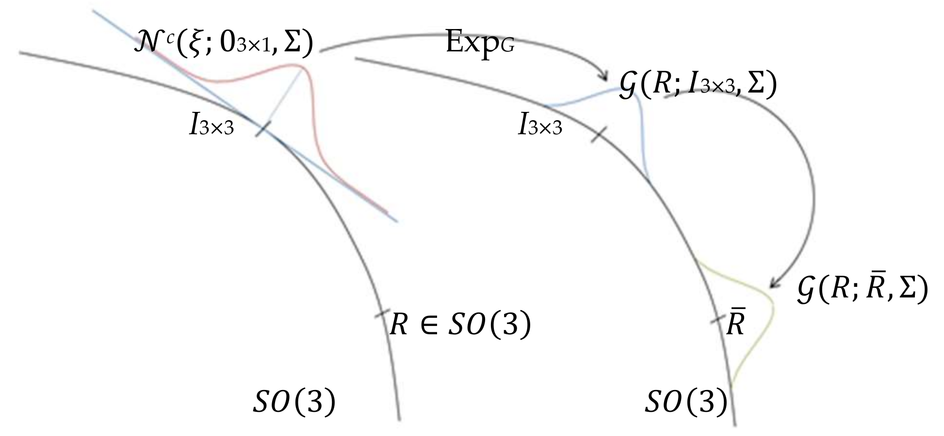
Figure 3.
Projecting the Lie groups model into vector space based on the invariant error.
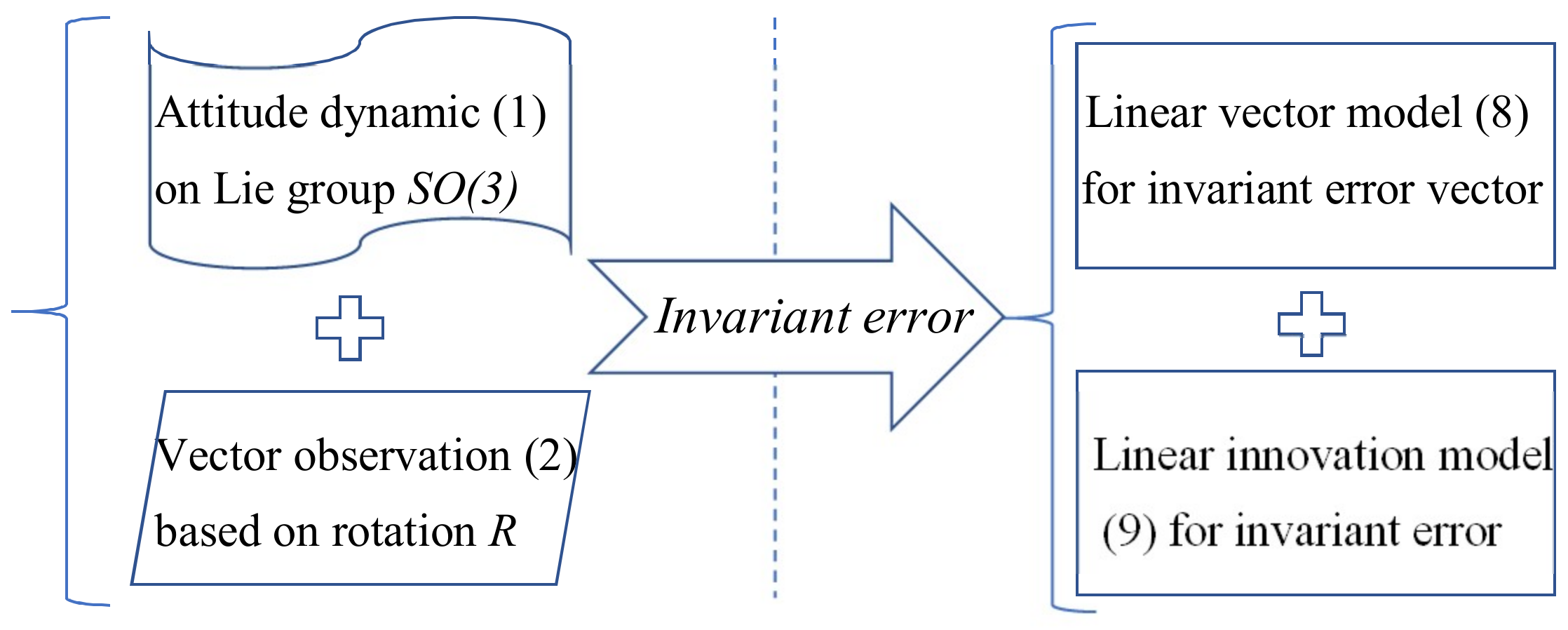
Figure 4.
The filtering diagram of the invariant Kalman filter for attitude estimation.
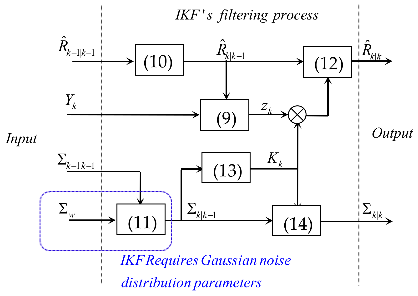
Figure 5.
The main idea and key innovation of this work to deal with the heavy-tailed attitude estimation problem on matrix Lie group SO(3).
Figure 5.
The main idea and key innovation of this work to deal with the heavy-tailed attitude estimation problem on matrix Lie group SO(3).
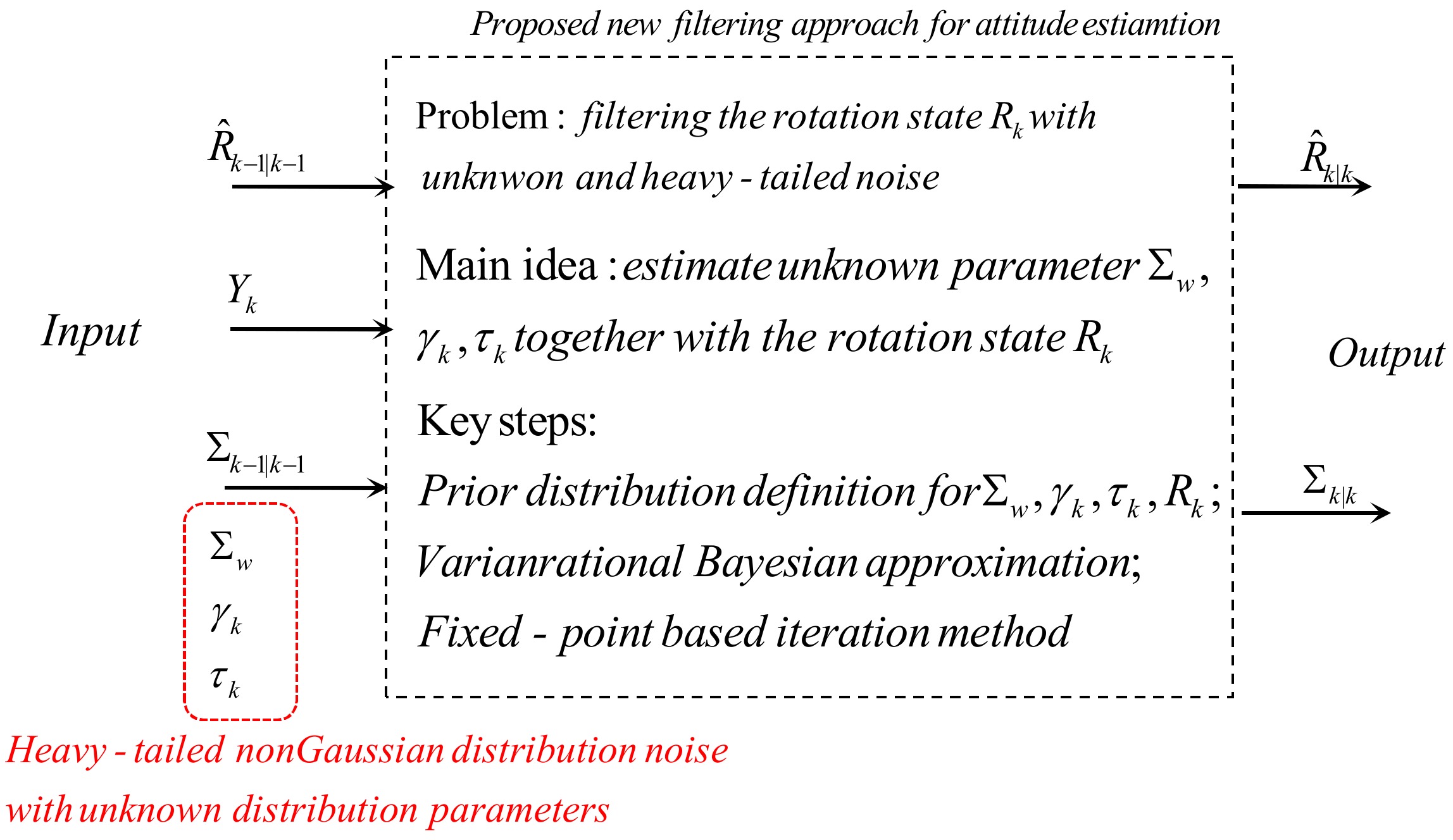
Figure 6.
Probability view of the proposed filtering method for Student’s t based hierarchical Gaussian state-space model.
Figure 6.
Probability view of the proposed filtering method for Student’s t based hierarchical Gaussian state-space model.

Figure 7.
The ARMSE result of RSIKF with different N for all cases of and .
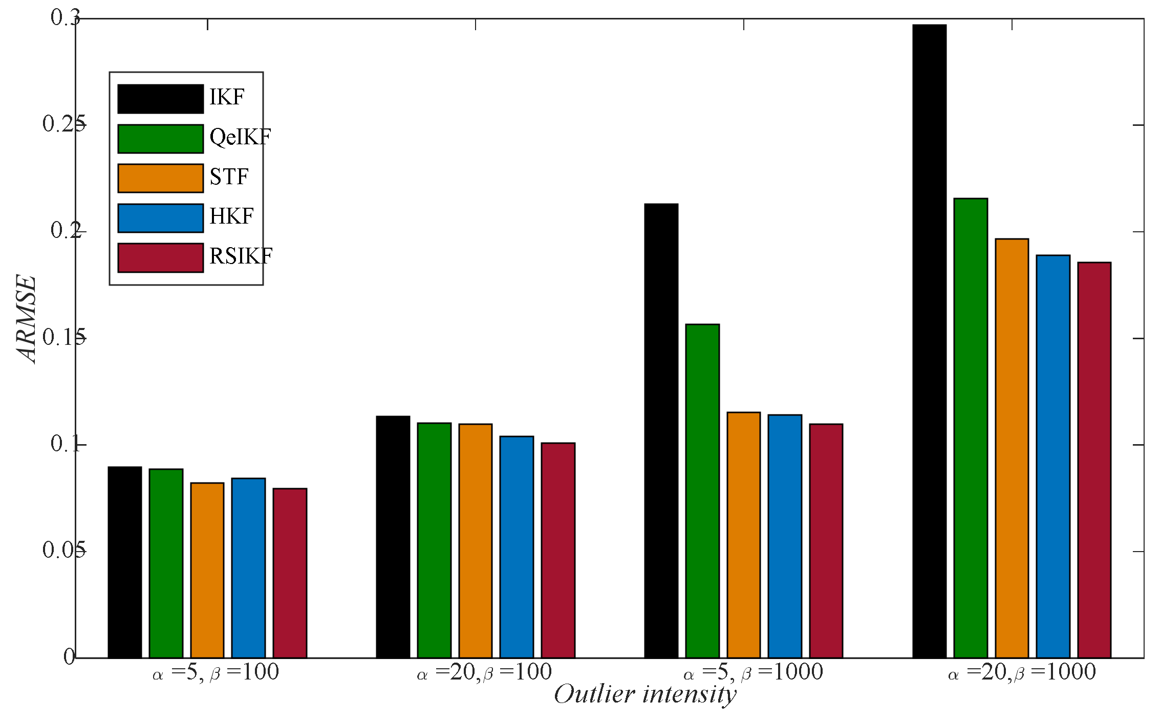
Figure 8.
The result of different methods for the case of = 5 and = 10.

Figure 9.
The result of different methods for the case of = 20 and = 10.
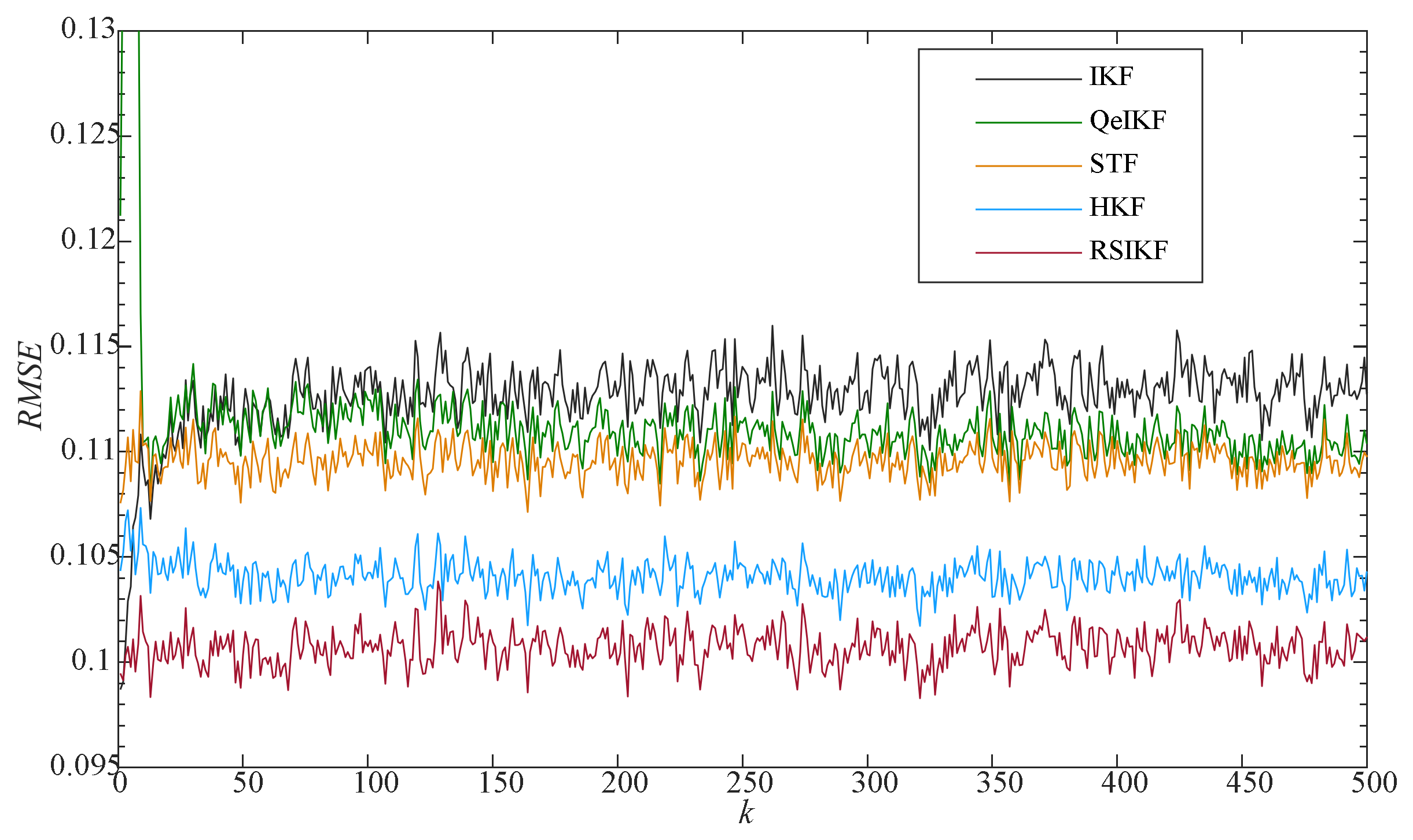
Figure 10.
The result of different methods for the case of = 5 and = 100.

Figure 11.
The result of different methods for the case of = 5 and = 100.
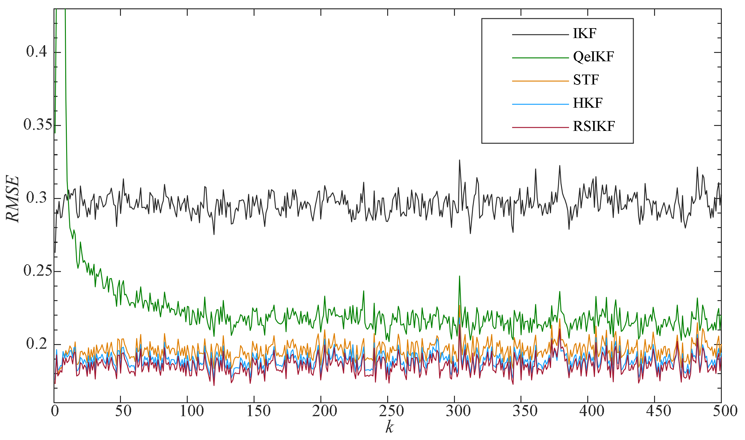
Figure 12.
The ARMSE result of RSIKF with different N for the cases of and .
Publisher’s Note: MDPI stays neutral with regard to jurisdictional claims in published maps and institutional affiliations. |
© 2021 by the authors. Licensee MDPI, Basel, Switzerland. This article is an open access article distributed under the terms and conditions of the Creative Commons Attribution (CC BY) license (https://creativecommons.org/licenses/by/4.0/).
Share and Cite
MDPI and ACS Style
Wang, J.; Zhang, C.; Wu, J.; Liu, M. An Improved Invariant Kalman Filter for Lie Groups Attitude Dynamics with Heavy-Tailed Process Noise. Machines 2021, 9, 182. https://doi.org/10.3390/machines9090182
AMA Style
Wang J, Zhang C, Wu J, Liu M. An Improved Invariant Kalman Filter for Lie Groups Attitude Dynamics with Heavy-Tailed Process Noise. Machines. 2021; 9(9):182. https://doi.org/10.3390/machines9090182
Chicago/Turabian StyleWang, Jiaolong, Chengxi Zhang, Jin Wu, and Ming Liu. 2021. "An Improved Invariant Kalman Filter for Lie Groups Attitude Dynamics with Heavy-Tailed Process Noise" Machines 9, no. 9: 182. https://doi.org/10.3390/machines9090182
Note that from the first issue of 2016, this journal uses article numbers instead of page numbers. See further details here.