Jets powered by black holes, which are then injected into the ambient interstellar medium, contain magnetic fields that are thought to be helically twisted (e.g., [
1]). On the basis of this understanding, we performed global simulations of jets containing helical magnetic fields injected into an ambient medium (e.g., [
5,
6]). The key issue we investigated was how the helical magnetic fields affect the growth of the kKHI, the MI, and the Weibel instability. RMHD simulations demonstrated that jets containing helical magnetic fields develop a kink instability (e.g., [
7,
8,
9]). Because our RPIC simulations were large enough to include a kink instability, we found a kink-like instability in our electron–proton jet case.
2.1. Helical Magnetic Field Structure
In our simulations [
5], cylindrical jets were injected with a helical magnetic field, implemented similarly to the RMHD simulations performed by Mizuno et al. [
10]. Our simulations used Cartesian coordinates. Because the pitch profile parameter
, which gives constant magnetic pitch and magnetic helicity, Equations (9)–(11) from [
10] are reduced to Equation (
1), and the magnetic field takes the following form:
The toroidal magnetic field is created by a current
in the positive
x-direction, so that it is defined in Cartesian coordinates by
Here
a is the characteristic length-scale of the helical magnetic field,
is the center of the jet, and
. The chosen helicity is defined through Equation (
2), which has a left-handed polarity with positive
. At the jet orifice, we implemented the helical magnetic field without the motional electric fields. This corresponded to a toroidal magnetic field generated self-consistently by jet particles moving along the
-direction.
2.2. Magnetic Fields in Helically Magnetized RPIC Jets with Larger Jet Radius
As an initial step, we examined how the helical magnetic field modifies the jet evolution using a small system before performing larger-scale simulations. A schematic of the simulation injection setup is given in our previous work [
5]. In these small-system simulations, we utilized a numerical grid with
(
L: simulation system length; simulation cell size:
) and periodic boundary conditions in transverse directions with a jet radius
. The jet and ambient (electron) plasma density measured in the simulation frame were
and
, respectively. This set of densities of jet and ambient plasmas was used in our previous simulations [
4,
5,
6].
In the simulations, the electron skin depth was , where c is the speed of light, is the electron plasma frequency, and the electron Debye length for the ambient electrons was . The jet-electron thermal velocity was in the jet reference frame. The electron thermal velocity in the ambient plasma was , and the ion thermal velocities were smaller by . The simulations were performed using an electron–positron () plasma or an electron–proton (– with ) plasma for the jet Lorentz factor of 15 and with the ambient plasma at rest ().
In the simulations, we used the initial magnetic field amplitude parameter (), the magnetization parameter defined as the ratio between the electromagnetic field (EMF) energy flux to the plasma matter energy flux , and the characteristic magnetic radius of . The helical field structure inside the jet was defined by Equations (1) and (2). For the external magnetic fields, we used a damping function that multiplies Equations (1) and (2) with the tapering parameter . The final profiles of the helical magnetic field components were similar to those of the case in which the jet radius was ; the only difference was that .
In this report, we maintain all the simulation parameters as described above, except the jet radius and simulation size (adjusted on the basis of the jet radius). We performed simulations with larger jet radii of
. In these small-system simulations, we utilized a numerical grid with
(simulation cell size:
). The cylindrical jet with jet radii of
was injected in the middle of the
y–
z plane (
, respectively) at
. The largest jet radius (
) was larger than that in [
4] (
), but the simulation length was much shorter (
).
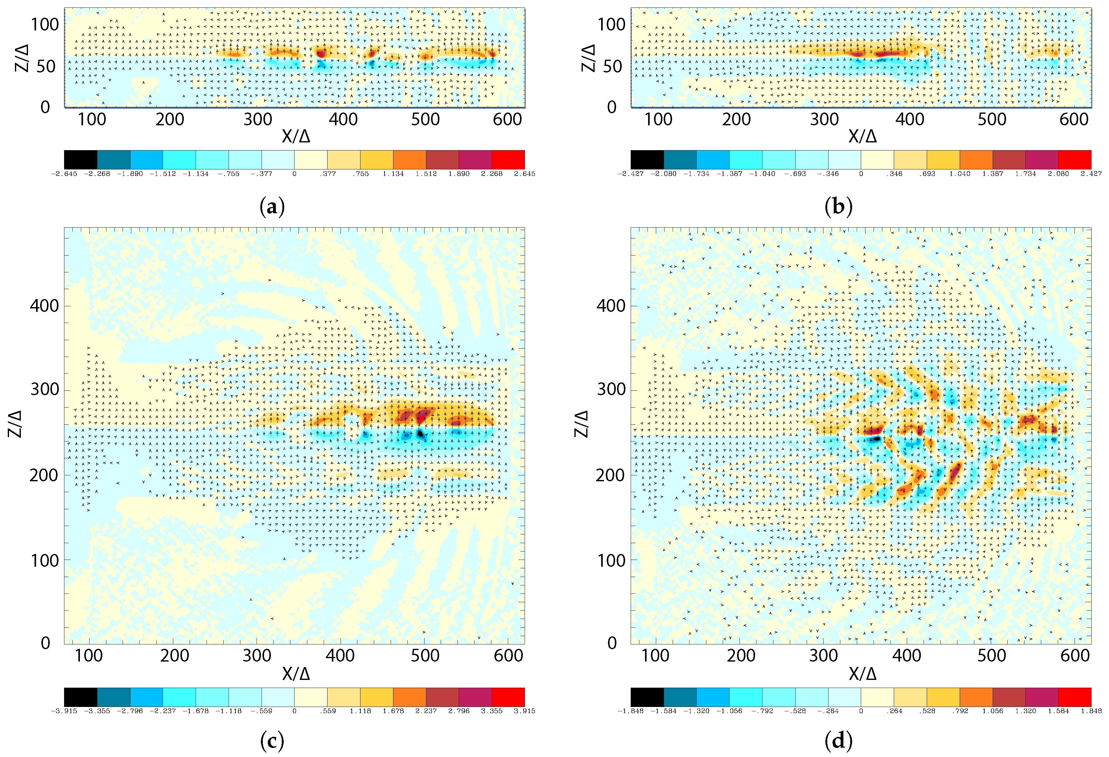
Figure 1 shows the
y-component of the magnetic field (
) in the jet radius with
. The initial helical magnetic field (left-handed; clockwise viewed from the jet front) was enhanced and disrupted as a result of the instabilities for both cases.
Even for shorter simulation systems, the growing instabilities were affected by the helical magnetic fields. These complicated patterns of
are generated by currents created by instabilities in jets. A larger jet radius provokes the growth of more modes of instabilities within jets, which make the jet structures more complicated. The simple recollimation shock generated in the small jet radius is shown in
Figure 1a,b [
5]. We need to perform longer simulations in order to investigate the full development of instabilities for jets with helical magnetic fields.
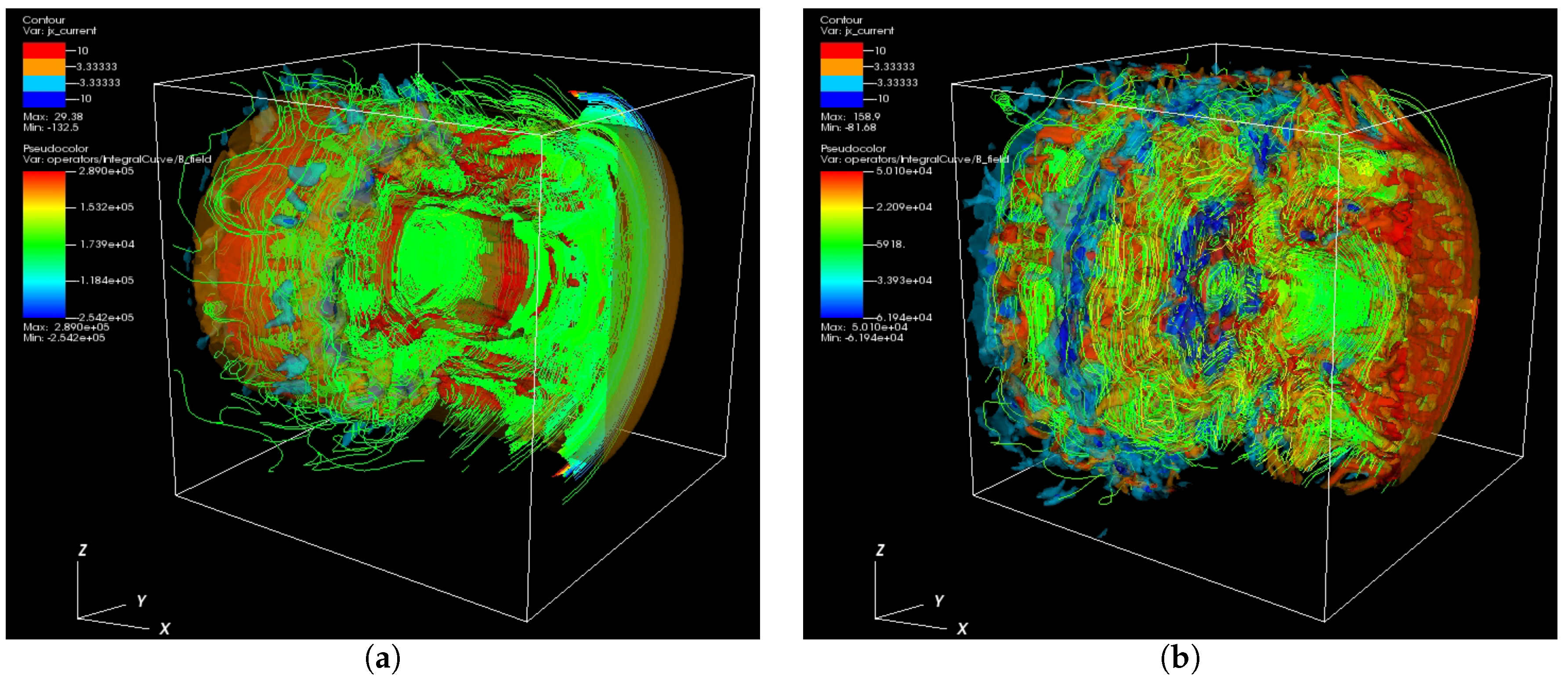
In order to investigate 3D structures of the averaged jet electron current (), we plotted it in the 3D (, , ) region of the jet front.
Figure 2 shows the current (
) of jet electrons for
–
(a) and
(b) jets. The cross-sections at
and the surfaces of jets show complicated patterns, which are generated by instabilities with the magnetic field lines.
In order to determine the particle acceleration, we calculated the Lorentz factor of jet electrons in the cases with
, as shown in
Figure 3. These patterns of the Lorentz factor coincided with the changing directions of local magnetic fields that were generated by instabilities. The directions of the magnetic fields are indicated by the arrows (black spots), which can be seen with magnification. The directions of the magnetic fields were determined by the generated instabilities. The structures at the edge of the jets were generated by the kKHI. The plots of the
x-component of the current
in the
y–
z plane show the MI in the circular edge of the jets, as shown in
Figure S1.
In order to investigate 3D structures of the averaged jet-electron Lorentz factor, we plotted its iso-surface (, ) of a quadrant of the jet front in 3D.
Figure 4 shows the Lorentz factor of jet electrons for
–
(a) and
(b) jets. The cross-sections and surfaces of the jets show complicated patterns that were generated by instabilities with the magnetic field lines.
In both cases with the jet radii larger than , the kKHI and MI were generated at the jet surfaces, and inside the jets, the Weibel instability was generated with kink-like instability, in particular in the electron–proton jet. We aim to investigate this further using different parameters, including a, which determines the structure of helical magnetic fields in Equations (1) and (2).


 ,
, 


