Static and Dynamic Characteristics of Rough Porous Rayleigh Step Bearing Lubricated with Couple Stress Fluid


Department of Mathematics, Gulbarga University, Kalaburagi 585106, India
*
Author to whom correspondence should be addressed.
Lubricants 2022, 10(10), 257; https://doi.org/10.3390/lubricants10100257
Submission received: 6 September 2022
/
Revised: 7 October 2022
/
Accepted: 10 October 2022
/
Published: 13 October 2022
(This article belongs to the Special Issue Tribological Characteristics of Bearing System)
Abstract
:In tribology, the Rayleigh step bearing has the maximum load capacity of any feasible bearing geometry. Traditional tribology resources have demonstrated that the Rayleigh step has an ideal geometry which maximizes load capacity. Both in nature and technology, rough and textured surfaces are essential for lubrication. While surface roughness enhances the performance of the bearings as an efficiency measure, it still has a significant impact on the load-carrying capacity of the bearing. In the present study, we investigate the dynamic characteristics of the Rayleigh step bearing with the impact of surface roughness and a porous medium by considering a squeezing action. Couple stress fluid is considered a lubricant with additives in both the film as well as the porous region. Based on Stokes constitutive equations for couple stress fluids, Darcy’s law for porous medium, and stochastic theory for rough surfaces, the averaged Reynolds-type equation is derived. Expressions are obtained for the volume flow rate, steady-state characteristics, and dynamic characteristics. The influence of surface roughness and the porous medium on the Rayleigh step bearing is analyzed. We investigated the static and dynamic characteristics of the Rayleigh step bearing. As a result, the couple stress fluid increases (decreases) the steady load-carrying capacity, dynamic stiffness, and dynamic damping coefficients, and decreases (increases) the volume flow rate negatively (positively) skewed roughness in comparison with that of the Newtonian case. The results are compared with those of the smooth case.
1. Introduction
In this paper, we analyzed the roughness influence on the dynamic behavior of porous Rayleigh Step Bearings (RSB) lubricated with couple stress fluids. The RSB is often used in industries because of its characteristics of higher Load Carrying Capacity (LCC). To improve LCC, much research has been conducted using an analytic method by solving the Reynolds equation. The concept of a step bearing was initially discussed by Lord Rayleigh [1] in 1918, who identified the ideal design with the highest load capacity per unit width for a specific film thickness and bearing length. This configuration is now referred to as the RSB. Since then, the characteristics of the RSB have been investigated by several researchers. Due to their high load capacity and cheap manufacturing costs, RSBs have been widely used in industries such as thrust bearings and pad bearings. In recent times, researchers have started studying non-Newtonian fluids, especially fluids containing additives or small particles, to analyze their effects on bearing performance, which the classical Newtonian theory failed to extend. The Stokes [2] Couple Stress Fluid is one such non-Newtonian fluid. Later, the use of porous bearings in the industry became widespread. A porous material is used in bearing systems to simplify production techniques, reduce costs, and extend service life. Porous bearings have a simple structure and are low cost. The application of porous bearings in mounting horsepower motors includes water pumps, vacuum cleaners, sewing machines, tape recorders, record players, shaving machines, coffee grinders, hair dryers, generators, and distributors. Bujurke et al. [3] considered a porous RSB lubricated by a second-order fluid and calculated the load capacity, frictional force, and frictional coefficients. Naduvinamani [4] theoretically presented double-layered porous RSBs with second-order fluid as a lubricant. Naduvinamani and Siddangouda [5] studied the optimum lubrication characteristics of porous RSBs lubricated with couple stress fluids. Later, they theoretically analyzed the lubrication characteristics of a porous inclined stepped composite bearing lubricated with micropolar fluid [6]. Rahmani et al. [7] described the effect of variations in pressure at the boundaries on the optimum properties of the RSB. Vakilian et al. [8] showed that inertia has a considerable effect on the thermohydrodynamic (THD) characteristics of step bearings having high-velocity runner surfaces. Naduvinamani et al. [9] obtained the optimum bearing parameters for the RSB lubricated with non-Newtonian Robinowitsch fluid. Shen et al. [10] investigated the flow characteristics in the Rayleigh step slider bearing with infinite width, both analytically and numerically. Alazwari et al. [11] analyzed the entropy optimization of first-grade viscoelastic nanofluid flow over a stretching sheet by using a classical Keller-box scheme. An analysis was carried out by Patel et al. [12] to enhance the performance of the ferrofluid lubricated porous step bearing by considering different flow models. Jamshed et al. [13] described the thermal efficiency enhancement of solar aircraft by utilizing unsteady hybrid nanofluid using a single-phase optimized entropy analysis. Muhammad Haq et al. [14] analyzed the energy transport of the magnetized forced flow of power-law nanofluid over a horizontal wall.
Surface roughness has a significant impact on bearing performance. Microscopic surface roughness is imposed on the surface during finishing processes such as grinding, lapping, and grit blasting. Christensen and Tonder [15] analyzed a stochastic method to study surface roughness. Andharia et al. [16] studied the impact of roughness on the performance of hydrodynamic slider bearings. Shiralashetti and Mounesha [17] used the wavelet-based decoupled method to investigate the effect of couple stress fluid and surface roughness on the elastohydrodynamic problem. Bijani et al. [18] studied the impact of surface texturing on the coefficient of friction in parallel sliding lubricated surfaces. Andharia and Pandya [19] considered the longitudinal roughness of the RSB. By adopting different porous structure models, Rao and Agarwal [20] analyzed the surface roughness effects on the hydrodynamic lubrication of step slider bearings. Paggi et al. [21] discussed the smoothed particle hydrodynamics (SPH) modeling of hydrodynamic lubrication along rough surfaces. Badescu [22] performed shape optimization of slider bearings operating with couple stress lubricants using a novel direct optimal control approach. Vashi et al. [23] scrutinized longitudinally rough, porous circular stepped plates with the impact of ferrofluid in the presence of couple stress. The deterministic mixed lubrication model was studied by Wang et al. [24] to understand the mechanism of LCC between parallel rough surfaces. Various researchers have recently begun investigating the bearings’ static and dynamic performance. Theoretically, Lin [25,26] presented the steady and dynamic performance of hydrostatic circular step thrust bearings with the effects of couple stresses, fluid inertia, and recess volume fluid compressibility and also derived a general Reynolds equation of sliding-squeezing surfaces with non-Newtonian fluids, which is necessary for assessment of the dynamic characteristics of a lubricating system. Lin et al. [27] studied the dynamic characteristics of an infinite-width tapered-land slider bearing by considering the squeezing action. The effect of couple stress fluid on the dynamic characteristics of wide exponential-shaped slider bearings and wide Rayleigh step slider bearings was presented by Lin et al. [28,29]. Naduvinamani and Patil [30] derived the dynamic Reynolds equation for micropolar fluid to study the dynamic characteristics of a finite exponential-shaped slider bearing. Singh and Gupta [31] theoretically investigated the effect of ferrofluid using the shliomis model on the dynamic characteristics of curved slider bearings. A theoretical study of the impact of roughness is analyzed by Siddangouda et. al. [32] on the static characteristics of an inclined plane slider-bearing lubricated with Rabinowitsch fluid. Rajeevkumar et al. [33] described the dynamic behavior of non-Newtonian power-law, micropolar, and couple stress fluids and their influence on the efficiency of journal bearings. Under the influence of micropolar fluid and roughness, the dynamic characteristics of inclined porous slider bearings are analyzed by Naduvinamani and Angadi [34]. Yandong Gu et al. [35] determined the static characteristics of aerostatic porous journal bearings theoretically and numerically. Fang et al. [36] discussed line contact stiffness and damping behaviors under transient elastohydrodynamic lubrication.
In this present paper, we studied the effect of porosity and roughness on the static and dynamic behavior of RSB lubricated with couple stress fluid along with squeezing action, on which a study has not been conducted so far as per the relevant literature known to the authors. An averaged modified Reynolds-type equation for rough porous RSBs has been derived and the numerical computations were carried out to get the required results. The probability density function (PDF) for the random variable is assumed to be asymmetrical with a non-zero mean, which characterizes the surface roughness.
2. Mathematical Formulation
Figure 1 represents the physical geometry of a rough porous RSB of length lubricated with Stokes non-Newtonian couple stress fluid [2]. The step bearing has a squeezing velocity and a sliding velocity . The film thickness can be described as
Here
where , is the outlet, inlet film thickness, is the difference between steady outlet-inlet film thickness and denotes the riser location parameter. This analysis assumes that the thin film theory of lubrication is applicable, and the body forces and body couples are absent. The Stokes [2] momentum and continuity equations for the couple stress fluid take the form,
where pressure and and are the fluid velocity components along and directions, respectively, in the film region, is the conventional shear viscosity, is a new material constant accounting for couple stresses and is of the dimension of momentum.
The relevant boundary conditions for the velocity components are
At
At
The velocity component in the direction and the dynamic Reynolds-type equation for non-Newtonian couple stress fluid can be obtained by solving Equations (3) and (5) subject to the relevant boundary conditions (6) and (7), and yields,
where is the molecular length of polar additives in a Newtonian fluid, which is given by and
The flow of couple stress fluid in the porous matrix is ruled by the modified Darcy’s law for porous material and is given by
where is the Darcy’s modified velocity vector, —permeability, and represents the ratio of the microstructure size to the pore size. If , i.e.,, then the microstructure additives present in the lubricant block the pores in the porous layer and thus reduce the Darcy flow through the porous matrix. When the microstructure size is very small compared to the pore size, i.e.,, the additives percolate into the porous matrix. Due to the continuity of the fluid in the porous matrix, the pressure satisfies the Laplace equation
Integration regarding over —the thickness of the porous layer, and utilizing the boundary condition at solid backing , we obtain
The assumption of small porous layer thickness and the utility of the pressure continuity condition at the porous interface deduce Equation (13) to
Then, at the interface , the velocity component is given by
Substituting Equation (15) in Equation (9), the dynamic Reynolds equation for couple stress fluid is acquired in the form
The Volume Flow Rate (VFR) in the direction can be evaluated by integrating the velocity component across the film thickness.
We can determine the VFR by performing the integration with the expression of .
Multiplying both sides of Equations (16) and (19) by and integrating with respect to over the interval and using as the mean, the standard deviation and the measure of symmetry of the random variable , the skewness parameter, where is the expectation operator defined by
The average Reynolds type equation is obtained in the form
where and is the expected value of
Adding the non-dimensional quantities
into Equations (21) and (22) gives the non-dimensional dynamic Reynolds equation and the volume flow rate in the form
where
and
The non-dimensional non-Newtonian couple stress dynamic Reynolds-type equation has two regions based on the geometry of the bearing.
For : Region 1
Here
For : Region 2
Here
and is the squeezing velocity in the non-dimensional form. The complimentary boundary conditions within Region 1 are:
Evaluating the volume flow rate (26) with the respective flow boundary condition (33) and solving the non-Newtonian dynamic Reynolds-type Equation (31) with the respective pressure boundary conditions (34) and (35), we obtain
where denotes the integration functions, and
The complimentary boundary conditions for Region 2 are:
Evaluation of the volume flow rate (26) with the corresponding flow boundary condition (40) and solution of the non-Newtonian dynamic Reynolds-type Equation (31) with the corresponding pressure boundary conditions (41) and (42) yields
where denotes the integration functions, and
Now at the position , equating the values of the VFR requires
Similarly, at the position , equating the values of the film pressure requires
Applying the conditions (38) and (39), we obtain the expressions of the integration functions.
The non-Newtonian dynamic film force can be evaluated by integrating film pressure over the fluid-film region. Expression of film force in a non-dimensional form is
By the use of the expression of the film pressure and performing the integrations, one can obtain the non-dimensional dynamic film force as
where the corresponding functions are defined in Appendix A. Following the similar procedures of the study of dynamic characteristics of wide RSB by Lin et al. [26], we can obtain the non-Newtonian steady VFR , non-Newtonian steady LCC , non-Newtonian Dynamic Stiffness Coefficient (DSC) and non-Newtonian Dynamic Damping Coefficient (DDC).
In the above equations, the subscript “s” denotes the bearing operating in a steady state. Appendix A defines various functions and quantities that are associated with various bearings. Using various bearing parameters,,, and are numerically computed and represented graphically. The simplified flowchart of the model is illustrated in Figure 2.
3. Results
The effect of non-Newtonian couple stress fluid and roughness on the dynamic characteristics of the porous RSB is analyzed. Based on the above analysis, the non-Newtonian couple stress parameter , the riser location parameter , the shoulder parameter , and roughness parameters are dominant in the RSB characteristics. As the permeability parameter and roughness parameters , the results obtained in the present article reduce to the case discussed by Lin et al. [26]. The values of the non-dimensional steady volume flow rate, steady LCC , DSC and DDC are calculated by using numerical computations.
3.1. Volume Flow Rate
The variation in the steady VFR as a function of the riser location parameter for different couple stress parameters and two distinct permeability parameters for , , , is represented in Figure 3. We observed that the required VFR increases with the increasing value of . Compared with the Newtonian case, the effect of couple stress lubricant provides further reductions in VFR. As compared with the smooth case and solid case, higher values of are noticed for the negatively skewed rough case. The effect of the porous layer increases the VFR with an increasing value of the permeability parameter . Figure 4 describes the varying values of as a function of for distinct values of the roughness parameter . For fixed values of , , , decreases for the negatively increasing value of and increases for the positively increasing value of when compared to the smooth case. The varying value of presented in Figure 5 is a function of for different values of with , , , . As increases, the VFR increases with the increasing value of the location parameter. The variation of with the location parameter for different values of with , , and is presented in Figure 6. We observed that the VFR increases for the increasing value of .
3.2. Steady Load-Carrying Capacity
Figure 7 depicts the variation of a non-dimensional steady LCC with the riser location parameter for distinct values of the couple stress parameters and with , , , . A higher steady LCC is obtained in the presence of non-Newtonian couple stresses for negatively skewed roughness as compared with the smooth case. The rough porous RSB lubricated with couple stress fluids has more LCC as compared with the corresponding Newtonian case. It is observed that the effect of the porous layer is to diminish the load capacity of the bearing as compared with the non-porous case; and also as the value of the permeability parameter increases, LCC decreases. Observing the Newtonian lubricant case, the steady LCC increases with the value of until a critical riser location is achieved, and thereafter falls as the value of continues to increase. For , the critical value . Figure 8, Figure 9 and Figure 10 describe the varying values of steady LCC with riser location parameter for various values of the roughness parameter , and , respectively. In Figure 8, the LCC increases for the negatively increasing value of and decreases for the positively increasing value . From Figure 9, it is evident that decreases for the increasing value of . Figure 10 clearly shows how the negatively increasing value of increases whereas the positively increasing value of decreases LCC .
3.3. Dynamic Stiffness Coefficient
Figure 11 represents the varying values of non-dimensional DSC with the riser location parameter and for distinct values of the couple stress parameter with , , , , . We observed higher DSC for increasing values of for negatively skewed roughness as compared with the smooth case. Compared with the Newtonian case, the effects of non-Newtonian couple stress fluid provide a higher bearing stiffness. The effect of permeability is to reduce the DSC as compared with the non-porous case. As the value of the permeability parameter increases, DSC decreases. We also observed the presence of the critical riser location parameter for the riser location parameter at which the DSC attains its maximum value. For , the critical value is . Figure 12, Figure 13 and Figure 14 denote the variation of non-dimensional DSC with riser location parameter for different values of the roughness parameters , and , respectively. Figure 12 shows that DSC increases for the negatively increasing value of whereas it decreases for the positively increasing values . From Figure 13, it is evident that decreases for the increasing value of . Figure 14 shows that the negatively increasing value of increases DSC whereas the positively increasing value of decreases DSC .
3.4. Dynamic Damping Coefficient
Figure 15 describes the variation in non-dimensional DDC as a function of the riser location parameter for different values of and under the shoulder parameter , roughness parameters . The damping coefficient is found to decrease with the increasing value of the riser location parameter and increase with the increasing value of the couple stress parameter . The RSB lubricated with couple stress fluids is observed to provide higher damping coefficients than Newtonian lubricants. As the permeability parameter decreases, DDC increases, and we also observed that DDC decreases with the increasing value of . The variation of non-dimensional DDC with for different values of , and are represented by Figure 16, Figure 17 and Figure 18, respectively. Figure 16 shows that DDC decreases with the increasing value of the location parameter , increases for the negatively increasing value of , and decreases for the positively increasing value of . From Figure 17, it is observed that decreases for the increasing value of .The negatively skewed roughness decreases whereas the positively skewed roughness decreases the DDC, as shown in Figure 18. Finally, on the whole, a small riser location parameter and a larger couple stress parameter improve the dynamic damping characteristics of the RSB.
The relative percentage increase due to the presence of couple stress fluid and porous medium in static and dynamic performance of a bearing is given by and where represents VFR, LCC, DSC and DDC.
Table 1 represents the static and dynamic behavior of rough porous RSB and its comparison with the non-porous rough surface. The values for porous rough RSB are tabulated for different values of the shoulder parameter and are compared with the non-porous rough RSB. Notably, when the steady inlet-outlet film thickness difference becomes zero, the step bearing becomes a parallel plate, so the volume flow rate is minimum, the static LCC and DSC are zero, and the DDC is maximum. As the shoulder parameter increases, the steady flow rate, LCC, and DSC increase until a certain point and then decrease as the value of increases.
Table 2 provides a numerical example to help with the selection of RSB lubricated with non-Newtonian couple stress fluid. The values for various bearing parameters are obtained. For engineering applications, RSB can be designed using the values obtained for physical quantities.
4. Conclusions
We studied the dynamic performance of rough porous RSB on the basis of Darcy’s law and Stokes micro-continuum theory. Based on the numerical computation of the results obtained and discussed, the following conclusions are drawn:
- The presence of microstructure additives in the lubricant enhances the LCC, DSC and DDC of the RSB and diminishes the VFR. There is a 7% decrease in VFR, and 14.12%, 16.06%, and 5.52%increase in LCC, DSC and DDC, respectively.
- The porous facing on the Rayleigh step slider bearing structure increases the VFR by 6.2% and decreases the LCC by 10.7%, DSC by 20.2% and DDC by 14.3%.
- The reduction in LCC caused by the porous facing can be compensated for by using lubricants that contain additives of the proper size. With this, bearing performance is enhanced.
- The presence of the negatively skewed surface roughness structure provides a reduction in the VFR, and higher steady LCC, DSC and DDC, whereas the positively skewed roughness enhances the VFR, and diminishes the load, stiffness, and damping coefficient.
- The presence of the surface roughness structure improves the LCC, DSC and DDC in comparison with the smooth surface case.
Compared with the non-porous smooth surface case of wide RSB by Lin et al. [26], a close agreement signifies support for the present study of the porous rough Rayleigh step bearing.
Author Contributions
Conceptualization, Supervision, Validation, Visualization, Writing—review & editing: N.N.; Formal analysis, Methodology, Visualization, Writing—original draft: A.A. All authors have read and agreed to the published version of the manuscript.
Funding
This research received no external funding.
Data Availability Statement
Not applicable.
Acknowledgments
The authors are thankful to the reviewers for their valuable comments on the earlier manuscripts, which were useful in enhancing the quality of this revised manuscript.
Conflicts of Interest
The authors declare no conflict of interest.
Nomenclature
| difference between the inlet-outlet film thicknesses, | |
| bearing width | |
| DDC, | |
| dynamic film force, | |
| integration functions, | |
| film thickness, | |
| inlet film thickness, | |
| steady inlet film thickness, | |
| outlet film thickness, | |
| steady outlet film thickness | |
| couple stress parameter, | |
| length of the bearing | |
| dynamic pressure, | |
| VFR, | |
| steady VFR, | |
| DSC, | |
| time, | |
| velocity components in the and directions | |
| sliding velocity of the lower part | |
| non-dimensional squeezing velocity, | |
| steady LCC, | |
| Cartesian coordinates | |
| non-dimensional coordinate, | |
| mean defined by | |
| riser location parameter | |
| shoulder parameter, | |
| skewness parameter defined by | |
| couple stress fluid material constant | |
| lubricant viscosity | |
| standard deviation defined by |
Appendix A
The Associated Functions and Quantities
References
- Lord Rayleigh, O.M.F.R.S. I. Notes on the theory of lubrication. Lond. Edinb. Dublin Philos. Mag. J. Sci. 1918, 35, 1–12. [Google Scholar] [CrossRef] [Green Version]
- Stokes, V.K. Couple stresses in fluids. Phys. Fluids 1966, 9, 1709. [Google Scholar] [CrossRef]
- Bujurke, N.M.; Naduvinamani, N.B.; Jagadeeswar, M. Porous Rayleigh step bearing with second-order fluid. J. Appl. Math. Mech. 1990, 70, 517–526. [Google Scholar] [CrossRef]
- Naduvinamani, N.B. Non-Newtonian effects of second-order fluids on double-layered porous Rayleigh-step bearings. Fluid Dyn. Res. 1997, 21, 495–507. [Google Scholar] [CrossRef]
- Naduvinamani, N.B.; Siddangouda, A. A note on porous Rayleigh step bearings lubricated with couple stress fluids. Proc. Inst. Mech. Eng. Part J J. Eng. Tribol. 2007, 221, 615–621. [Google Scholar] [CrossRef]
- Naduvinamani, N.B.; Siddangouda, A. Porous inclined stepped composite bearings with micropolar fluid. Tribol.-Mater. Surf. Interfaces 2007, 1, 224–232. [Google Scholar] [CrossRef]
- Rahmani, R.; Shirvani, A.; Shirvani, H. Analytical analysis and optimization of the Rayleigh step slider bearing. Tribol. Int. 2009, 42, 666–674. [Google Scholar] [CrossRef] [Green Version]
- Vakilian, M.; Nassab, S.A.G.; Kheirandish, Z. Study of inertia effect on thermohydrodynamic characteristics of Rayleigh step bearings by CFD method. Mech. Ind. 2013, 14, 275–285. [Google Scholar] [CrossRef]
- Naduvinamani, N.B.; Patil, S.; Siddapur, S.S. On the study of Rayleigh step slider bearings lubricated with non-Newtonian Robinowitsch fluid. Ind. Lubr. Tribol. 2017, 69, 666–672. [Google Scholar] [CrossRef]
- Shen, F.; Yan, C.J.; Dai, J.F.; Liu, Z.M. Recirculation flow and pressure distributions in a Rayleigh step bearing. Adv. Tribol. 2018, 2018, 9480636. [Google Scholar] [CrossRef]
- Alazwari, M.A.; Nidal, H.A.; Goodarzi, M. Entropy optimization of first-grade viscoelastic Nanofluid flow over a stretching sheet by using classical Keller-Box scheme. Mathematics 2021, 9, 2563. [Google Scholar] [CrossRef]
- Patel, D.A.; Joshi, M.; Patel, D.B. Design of porous step bearing by considering different ferro fluid lubrication flow model. J. Manuf. Eng. 2021, 16, 108–114. [Google Scholar] [CrossRef]
- Jamshed, W.; Alanazi, A.K.; Isa, S.S.P.M.; Banerjee, R.; Eid, M.R.; Nisar, K.S.; Alshahrei, H.; Goodarzi, M. Thermal efficiency enhancement of solar aircraft by utilizing unsteady hybrid nanofluid: A single-phase optimized entropy analysis. Sustain. Energy Technol. Assess. 2022, 52, 101898. [Google Scholar] [CrossRef]
- ul Haq, M.R.; Hussain, M.; Bibi, N.; Shigidi, I.M.T.A.; Pashameah, R.A.; Alzahrani, E.; El-Shorbagy, M.A.; Safaei, M.R. Energy transport analysis of the magnetized forced flow of power-law nanofluid over a horizontal wall. J. Magn. Magn. Mater. 2022, 560, 169681. [Google Scholar] [CrossRef]
- Christensen, H. Stochastic models of hydrodynamic lubrication of rough surfaces. Proc. Inst. Mech. Eng. 1969, 184, 1013–1026. [Google Scholar] [CrossRef]
- Andharia, P.I.; Gupta, J.L.; Deheri, G.M. Effect of surface roughness on hydrodynamic lubrication of slider bearings. Tribol. Trans. 2001, 44, 291–297. [Google Scholar] [CrossRef]
- Shiralashetti, S.C.; Kantli, M.H. Investigation of Couple Stress Fluid and Surface Roughness Effects in the Elastohydrodynamic Lubrication Problems using Wavelet-Based Decoupled Method. Lubricants 2016, 4, 9. [Google Scholar] [CrossRef] [Green Version]
- Dariush, B.; Deladi, E.L.; Aydar, A.; Matthijn, R.; Dirk, S. The Influence of Surface Texturing on the Frictional Behaviour of Parallel Sliding Lubricated Surfaces under Conditions of Mixed Lubrication. Lubricants 2018, 6, 91. [Google Scholar] [CrossRef] [Green Version]
- Andharia, P.I.; Pandya, H.M. Effect of Longitudinal Surface Roughness on the performance of RSB. Int. J. Appl. Eng. Res. 2018, 13, 14935–14941. Available online: https://www.ripublication.com/ijaer18/ijaerv13n21_17.pdf (accessed on 8 July 2021).
- Rao, P.S.; Agarwal, S. Theoretical study of couple stress fluid film in rough step slider bearing with assorted porous structure. J. Nanofluids 2018, 7, 92–99. [Google Scholar] [CrossRef]
- Marco, P.; Andrea, A.; Pietro, L. SPH Modeling of Hydrodynamic Lubrication along Rough Surfaces. Lubricants 2019, 7, 103. [Google Scholar] [CrossRef]
- Badescu, V. Two classes of sub-optimal shapes for one dimensional slider bearings with couple stress lubricants. Appl. Math. Model. 2020, 81, 887–909. [Google Scholar] [CrossRef]
- Vashi, Y.D.; Patel, R.M.; Deheri, G.B. Neuringer-Roseinweig model based longitudinally rough porous circular stepped plates in the existence of couple stress. Acta Polytech. 2020, 30, 259–267. [Google Scholar] [CrossRef]
- Wang, Y.; Azam, A.; Zhang, G.; Dorgham, A.; Liu, Y.; Wilson, M.C.T.; Neville, A. Understanding the Mechanism of Load-Carrying Capacity between Parallel Rough Surfaces through a Deterministic Mixed Lubrication Model. Lubricants 2022, 10, 12. [Google Scholar] [CrossRef]
- Lin, J.R. Static and dynamic behavior of externally pressurized circular step thrust bearings lubricated with couple stress fluids. Tribol. Int. 1999, 32, 207–216. [Google Scholar] [CrossRef]
- Lin, J.R.; Lu, R.F.; Chang, T.B. Derivation of Dynamic couple-stress Reynolds equation of sliding-squeezing surfaces and Numerical Solution of Plane Inclined Slider Bearings. Tribol. Int. 2003, 36, 679–685. [Google Scholar] [CrossRef]
- Lin, J.R.; Lu, R.-F.; Ho, M.-H.; Lin, M.-C. Dynamic characteristics of wide tapered-land slider bearings. J. Chin. Inst. Eng. 2006, 29, 543–548. [Google Scholar] [CrossRef]
- Lin, J.R.; Lu, R.F.; Ho, M.H.; Li, M.C. Dynamic characteristics of wide exponential film-shape slider bearings lubricated with a non-Newtonian couple stress fluid. J. Mar. Sci. Technol. 2006, 14, 93–101. [Google Scholar] [CrossRef]
- Lin, J.-R.; Chu, L.M.; Liaw, W.-L. Effects of non-Newtonian couple stress on the dynamic characteristics of wide Rayleigh step slider bearings. J. Mar. Sci. Technol. 2012, 20, 9. [Google Scholar] [CrossRef]
- Naduvinamani, N.B.; Patil, S.B. Static and dynamic characteristics of finite exponential film shaped slider bearings lubricated with micropolar fluid. Tribol.-Mater. Surf. Interfaces 2009, 3, 110–117. [Google Scholar] [CrossRef]
- Singh, U.P.; Gupta, R.S. Dynamic performance characteristics of a curved slider bearing operating with ferrofluids. Adv. Tribol. 2012, 2012, 278723. [Google Scholar] [CrossRef]
- Siddangouda, A.; Naduvinamani, N.B.; Siddapur, S.S. Effect of surface roughness on the static characteristics of inclined plane slider bearing: Rabinowitsch fluid model. Tribol.-Mater. Surf. Interfaces 2017, 11, 125–135. [Google Scholar] [CrossRef]
- Dang, R.K.; Goyal, D.; Chauhan, A.; Dhami, S.S. Effect of non-Newtonian lubricants on static and dynamic characteristics of journal bearings. Mater. Today Proc. 2020, 28, 1345–1349. [Google Scholar] [CrossRef]
- Naduvinamani, N.B.; Ashwini, A. On the dynamic characteristics of rough porous inclined slider bearing lubricated with micropolar fluid. Tribol. Online 2022, 17, 59–70. [Google Scholar] [CrossRef]
- Gu, Y.; Cheng, J.; Xie, C.; Li, L.; Zheng, C. Theoretical and Numerical Investigations on Static Characteristics of Aerostatic Porous Journal Bearings. Machines 2022, 10, 171. [Google Scholar] [CrossRef]
- Fang, C.; Zhu, A.; Zhou, W.; Peng, Y.; Meng, X. On the Stiffness and Damping Characteristics of Line Contacts under Transient Elastohydrodynamic Lubrication. Lubricants 2022, 10, 73. [Google Scholar] [CrossRef]
Figure 1.
Physical geometry of the considered problem.
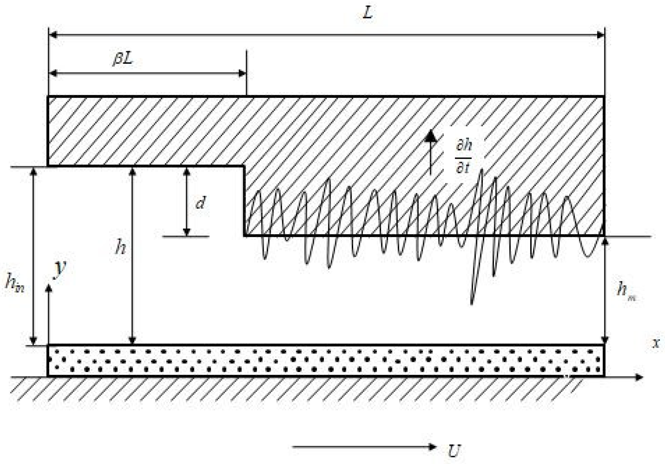
Figure 2.
Flow chart of the numerical model.

Figure 3.
Steady volume flow rate as a function of for different and under .

Figure 4.
Steady volume flow rate as a function of for different under .

Figure 5.
Steady volume flow rate as a function of for different under .
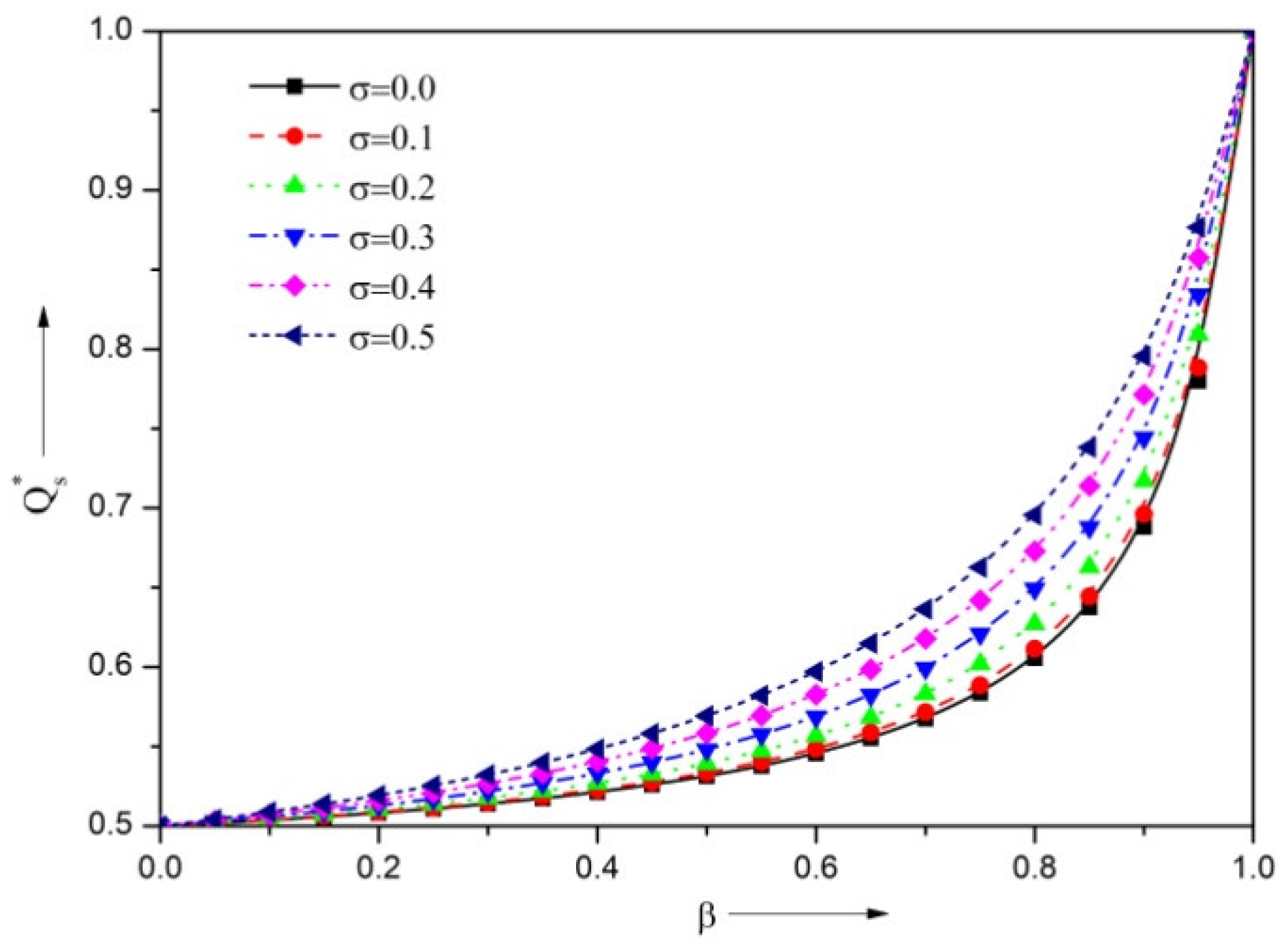
Figure 6.
Steady volume flow rate as a function of for different under .
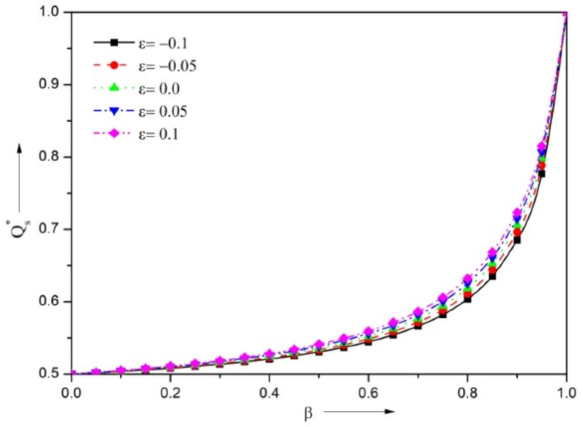
Figure 7.
Steady load-carrying capacity as a function of for different and under .
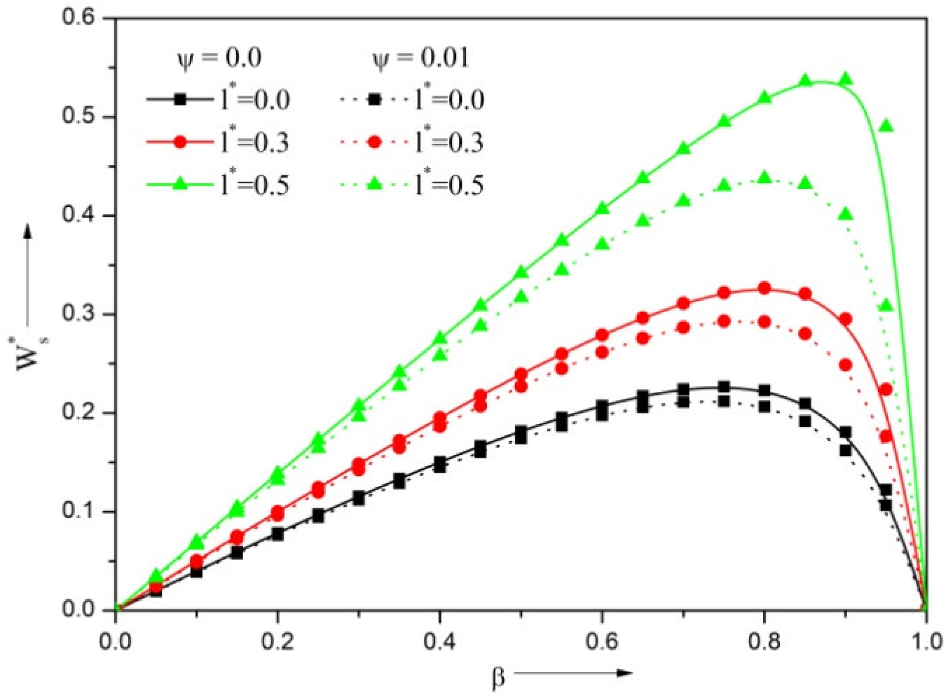
Figure 8.
Steady load-carrying capacity as a function of for different under .
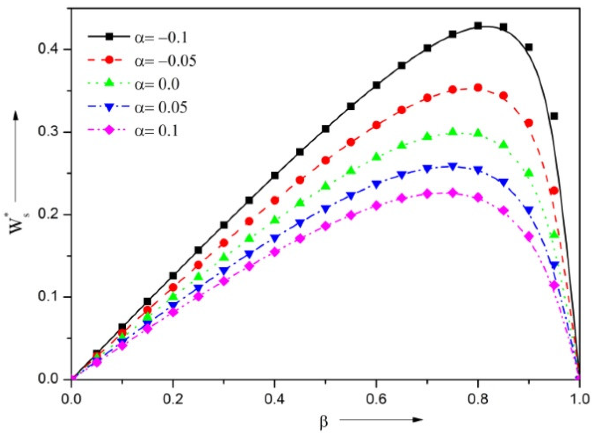
Figure 9.
Steady load-carrying capacity as a function of for different under .
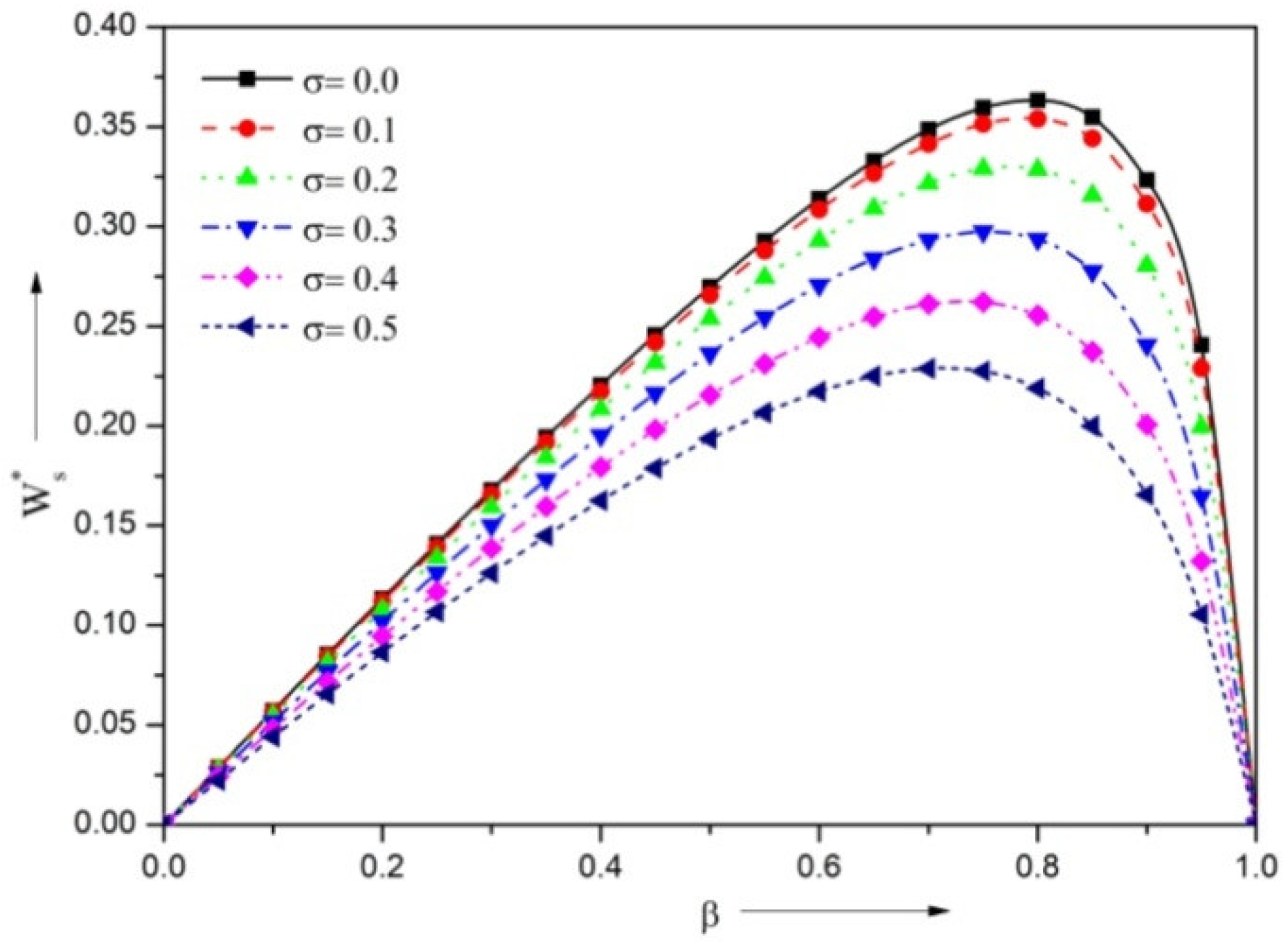
Figure 10.
Steady load-carrying capacity as a function of for different under .
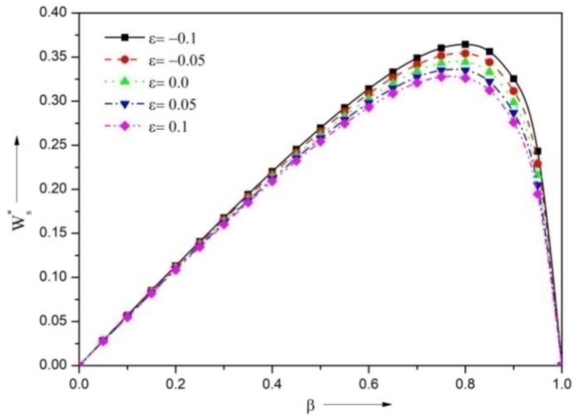
Figure 11.
Dynamic stiffness coefficient as a function of for different and under .
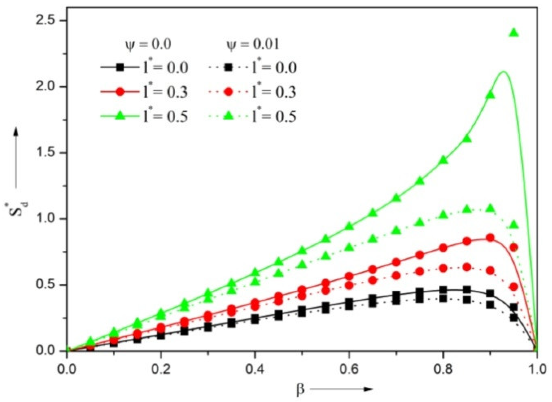
Figure 12.
Dynamic stiffness coefficient as a function of for different under .
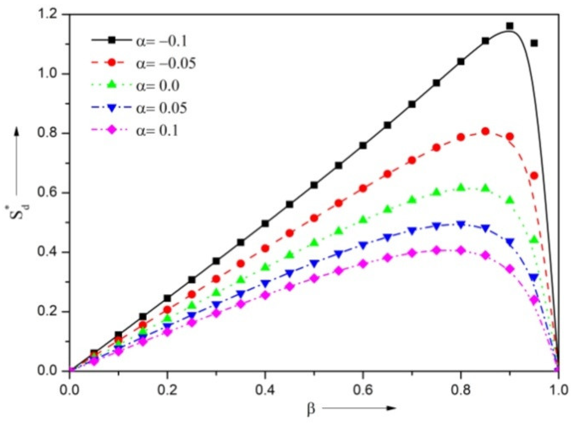
Figure 13.
Dynamic stiffness coefficient as a function of for different under .
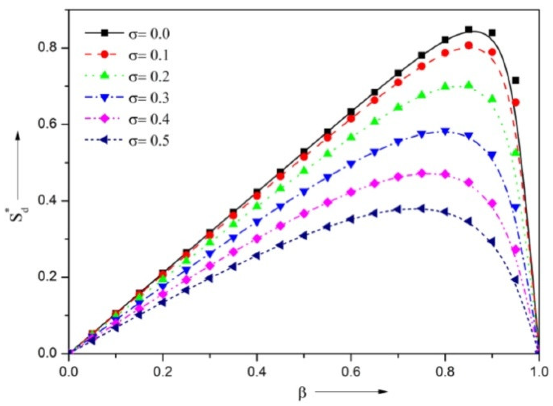
Figure 14.
Dynamic stiffness coefficient as a function of for different under .

Figure 15.
Dynamic damping coefficient as a function of for different and under .

Figure 16.
Dynamic damping coefficient as a function of for different under .
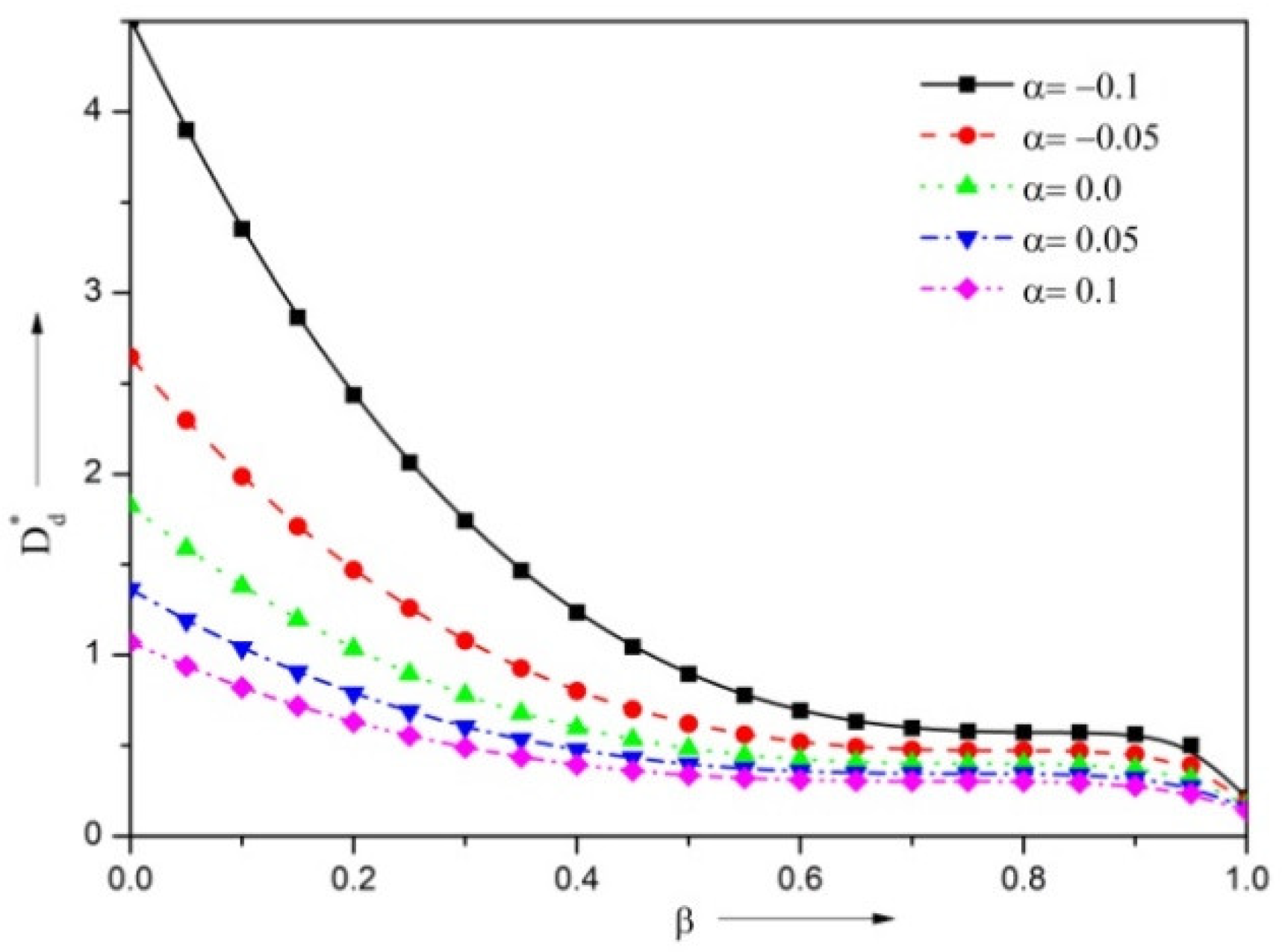
Figure 17.
Dynamic damping coefficient as a function of for different under .
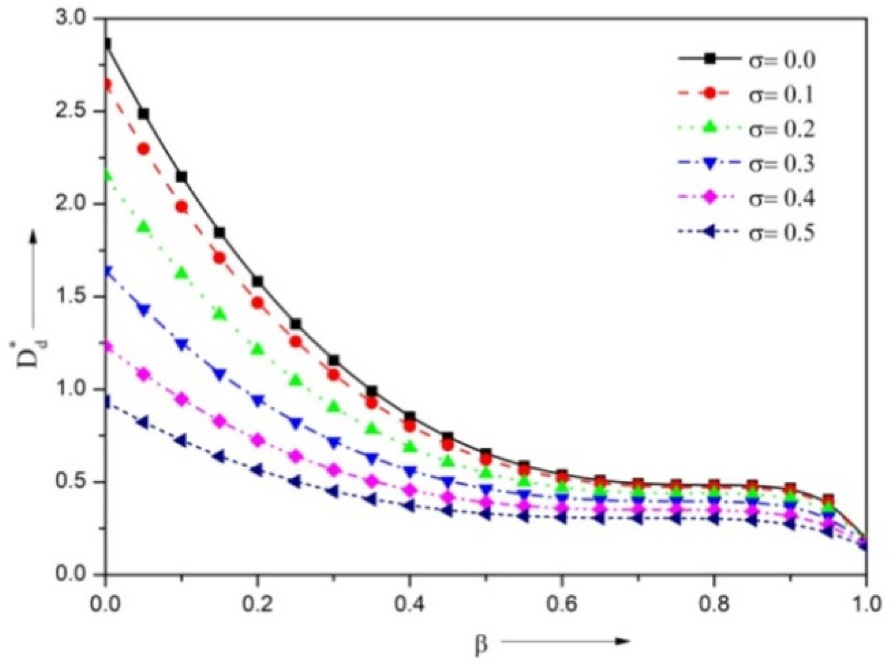
Figure 18.
Dynamic damping coefficient as a function of for different under .


Table 1.
Static and dynamic characteristics of porous rough RSB and its comparison with non-porous rough surface.
Table 1.
Static and dynamic characteristics of porous rough RSB and its comparison with non-porous rough surface.
| Non-Porous Rough Surface | Porous Rough Surface | Non-Porous Rough Surface | Porous Rough Surface | ||||||
|---|---|---|---|---|---|---|---|---|---|
| NSSR | PSSR | NSSR | PSSR | NSSR | PSSR | NSSR | PSSR | ||
| 0 | 0.5 | 0.5 | 0.5 | 0.5 | 0.5 | 0.5 | 0.5 | 0.5 | |
| 0.5 | 0.612961 | 0.623292 | 0.621158 | 0.628646 | 0.569021 | 0.610331 | 0.596764 | 0.620916 | |
| 1 | 0.626252 | 0.649364 | 0.642319 | 0.661148 | 0.554155 | 0.61458 | 0.588517 | 0.634438 | |
| 1.5 | 0.609108 | 0.636499 | 0.626454 | 0.650336 | 0.538447 | 0.593059 | 0.5666 | 0.613143 | |
| 2 | 0.588865 | 0.615334 | 0.604549 | 0.628555 | 0.528012 | 0.572678 | 0.549736 | 0.589958 | |
| 2.5 | 0.571852 | 0.595586 | 0.585248 | 0.607297 | 0.521175 | 0.557179 | 0.538049 | 0.57145 | |
| 3 | 0.558584 | 0.579297 | 0.569853 | 0.589395 | 0.516534 | 0.545788 | 0.529902 | 0.557526 | |
| 0 | 0 | 0 | 0 | 0 | 0 | 0 | 0 | 0 | |
| 0.5 | 0.202712 | 0.149249 | 0.18042 | 0.136804 | 0.501619 | 0.260817 | 0.384162 | 0.253665 | |
| 1 | 0.226563 | 0.18081 | 0.21193 | 0.171367 | 0.393575 | 0.270861 | 0.351423 | 0.281003 | |
| 1.5 | 0.195797 | 0.165237 | 0.188306 | 0.15987 | 0.279421 | 0.219986 | 0.26441 | 0.231931 | |
| 2 | 0.15947 | 0.139615 | 0.155687 | 0.136707 | 0.203581 | 0.171807 | 0.197455 | 0.180856 | |
| 2.5 | 0.128941 | 0.11571 | 0.126945 | 0.114101 | 0.153891 | 0.135169 | 0.151057 | 0.141432 | |
| 3 | 0.10513 | 0.095991 | 0.104019 | 0.095064 | 0.120164 | 0.108241 | 0.118714 | 0.112535 | |
| 0 | 0 | 0 | 0 | 0 | 0 | 0 | 0 | 0 | |
| 0.5 | 0.531458 | 0.341553 | 0.420996 | 0.286967 | 1.95344 | 0.682152 | 1.14572 | 0.507848 | |
| 1 | 0.44829 | 0.329102 | 0.392252 | 0.295624 | 0.943611 | 0.540175 | 0.752312 | 0.460935 | |
| 1.5 | 0.298172 | 0.239054 | 0.275793 | 0.223777 | 0.46872 | 0.335988 | 0.419848 | 0.307854 | |
| 2 | 0.194121 | 0.164385 | 0.185019 | 0.157608 | 0.261167 | 0.208737 | 0.245687 | 0.198222 | |
| 2.5 | 0.129902 | 0.113895 | 0.125912 | 0.110748 | 0.159793 | 0.135509 | 0.153962 | 0.131151 | |
| 3 | 0.0901384 | 0.080881 | 0.0882435 | 0.079326 | 0.104931 | 0.092197 | 0.102416 | 0.090203 | |
| 0 | 1.19635 | 0.807021 | 0.992749 | 0.708942 | 4.84507 | 1.57596 | 2.64674 | 1.24076 | |
| 0.5 | 0.562794 | 0.421535 | 0.507631 | 0.39037 | 1.33879 | 0.721327 | 1.04471 | 0.632911 | |
| 1 | 0.302087 | 0.241763 | 0.28299 | 0.229856 | 0.552039 | 0.36137 | 0.472845 | 0.33376 | |
| 1.5 | 0.177866 | 0.148018 | 0.169361 | 0.142651 | 0.2988 | 0.202675 | 0.253901 | 0.190768 | |
| 2 | 0.114836 | 0.097212 | 0.109655 | 0.094137 | 0.19713 | 0.127897 | 0.159563 | 0.120346 | |
| 2.5 | 0.0805295 | 0.068291 | 0.0765075 | 0.066079 | 0.149001 | 0.089316 | 0.113463 | 0.083156 | |
| 3 | 0.0605741 | 0.050941 | 0.0570036 | 0.049083 | 0.123353 | 0.067683 | 0.0884973 | 0.062033 | |
NSSR: Negatively Skewed Surface Roughness, PSSR: Positively Skewed Surface Roughness.
Table 2.
Design example of rough Rayleigh step bearing with couple stress fluid.
| Physical Quantity | Symbol | Value of the Physical Quantity |
|---|---|---|
| Bearing length | ||
| Inlet film thickness | ||
| Steady outlet film thickness | ||
| Length of the first part of the bearing | ||
| Lubricant viscosity | ||
| Shoulder parameter | ||
| Riser location parameter | ||
| Couple stress parameter | ||
| Couple stress material constant | ||
| Roughness parameters | −0.05 | |
| 0.1 | ||
| −0.05 |
Publisher’s Note: MDPI stays neutral with regard to jurisdictional claims in published maps and institutional affiliations. |
© 2022 by the authors. Licensee MDPI, Basel, Switzerland. This article is an open access article distributed under the terms and conditions of the Creative Commons Attribution (CC BY) license (https://creativecommons.org/licenses/by/4.0/).
Share and Cite
MDPI and ACS Style
Naduvinamani, N.; Angadi, A. Static and Dynamic Characteristics of Rough Porous Rayleigh Step Bearing Lubricated with Couple Stress Fluid. Lubricants 2022, 10, 257. https://doi.org/10.3390/lubricants10100257
AMA Style
Naduvinamani N, Angadi A. Static and Dynamic Characteristics of Rough Porous Rayleigh Step Bearing Lubricated with Couple Stress Fluid. Lubricants. 2022; 10(10):257. https://doi.org/10.3390/lubricants10100257
Chicago/Turabian StyleNaduvinamani, Neminath, and Ashwini Angadi. 2022. "Static and Dynamic Characteristics of Rough Porous Rayleigh Step Bearing Lubricated with Couple Stress Fluid" Lubricants 10, no. 10: 257. https://doi.org/10.3390/lubricants10100257
Note that from the first issue of 2016, this journal uses article numbers instead of page numbers. See further details here.