Mixed Lubrication Analysis of Tapered Roller Bearings and Crowning Profile Optimization Based on Numerical Running-In Method

Abstract

Tapered roller bearings (TRBs) are widely used in heavy-load rotating machinery. One of the technical problems in TRBs is the existence of sharp spikes of the contact pressure in the vicinity of the two ends of the tapered rollers. To suppress the pressure spikes at the roller ends, a straight roller profile is crowned in cylindrical and tapered roller bearings. However, compared to cylindrical roller bearings, there are few studies on the profile modification of TRBs in the literature, and most of the publications on the EHD analysis of tapered rollers focused on a single roller, using traditional profiles such as logarithmic profiles, dub-off profiles and chamfer profiles. By using the numerical running-in method proposed and used in crowning profiles of cylindrical rollers by the authors, this paper provides the first ever asymmetric optimized profile solution for all TRBs rather than for just a single roller. The results show that the optimized profile has the best performance in smoothing contact pressure distribution in the axial direction compared with the conventional logarithmic profile and is a useful profile form with respect to the elimination of sharp pressure spikes. In addition, considering the effect of temperature and mixed lubrication, this paper analyzes the influences of different axial profiles under radial load (Fr), rotation speed (N) and standard deviation of roughness (Rq) conditions.

1. Introduction

Among many types of rolling element bearings, tapered roller bearings (TRB) are advantageous to operate under combined heavy radial and thrust loadings, and hence are widely used in rotating machinery, such as helicopter gearboxes, high-speed railway train axle boxes, wind turbines’ main shafts and so on.

Over the decades, the numerical modeling of rolling element bearings has attracted significant attention [1,2,3]. Compared with other types of rolling element bearings, analyses of the kinematic and friction behavior of TRBs are more difficult due to their complex geometric structure. Therefore, in the literature, there are relatively few reports on TRB dynamics and elastohydrodynamic lubrication (EHL). Rahnejat and Gohar [4] reported the influence of misalignment to the radial contact pressure distributions on tapered rollers. They suggested careful axial profiling is important. Cretu et al. [5,6] developed a comprehensive dynamic model to analyze TRBs with six degrees of freedom. In addition to complex loads, the quasi-dynamic model considered centrifugal forces and roller gyroscopic moments. To obtain the film thickness and pressure distributions between tapered rollers and raceways, Yamashita et al. [7] presented an approximate fluid film lubrication model, which combined a quasi-static model and a raceway EHL model. In recent years, Zheng et al. [8] used a quasi-static model to investigate the influences of angular misalignment and frictional force on contact pressure distributions of the main shaft bearing installed in a modern wind turbine. Zhang et al. [9] explored the effects of roller skewing on the frictional torque of a dry-lubricated tapered roller bearing. Nguyen-Schaefer [10] presented a computational model consisting of many circular slices per rolling element of rollers in the TRB and applied the Levenberg–Marquardt’s algorithm to solve the strongly nonlinear coupled equation systems. However, all of the studies mentioned above were carried out without considering the mixed lubrication of rollers in the TRB.

Considering the increasingly harsh working conditions of tapered roller bearings, investigating the mixed lubrication of finite line contacts has become more and more significant in recent years. The foundation of the line contact EHL theory has been paved by Petrusevich [11], Dowson and Higginson [12] and many others, including Gohar and Cameron [13] and Wymer and Cameron [14]. Bahadoran and Gohar [15] investigated the effects of different geometries of rollers on the EHL characteristics through experimental measurements, and they found that the film thickness is contractive near the roller ends. Kushwaha et al. [16,17] provided the EHL solutions of aligned and misaligned finite line contact. Then, they discussed the effect of transient conditions. Liu and Yang [18] developed the thermal EHL of finite line contacts under heavy loads. Based on the thermal EHL model, Yang and Yang [19] studied the lubrication performances of two tapered rollers located in the opposite orientations. Zhu et al. [20] presented a mixed EHL investigation considering realistic geometries (crowning, end corners and chamfers) and surface roughness effects on the behavior of finite line contact. Patir and Cheng [21,22] proposed the well-known average flow model to modify the Reynolds equation, which can consider the effect of surface roughness on lubrication performance. Then, Kogut and Etsion [23,24,25] presented the elastic–plastic model (KE model), which can calculate the asperity contact pressure in a statistic manner. Associated with this research into finite line contact and mixed lubrication, the modification of roller profiles has been studied and improved to reduce the end effect of stress concentration.

The famous logarithmic function to modify axial profile was introduced by Lundberg [26] in 1939. It can achieve the uniform pressure distribution of finite line contacts on the assumption of dry, static and elastic contact. Then, Johns and Gohar [27] improved Lundberg’s function, and Fujiwara [28,29] put forward an optimized logarithmic profile. Cui and He [30] found a new logarithmic profile model of cylindrical roller bearings, which can avoid edge effects and increase the fatigue life of cylindrical roller bearings. Except for the logarithmic profile, the effects of other different types of profiles have also been investigated. Poplawski et al. [31] analyzed and compared four common roller profiles (flat roller profile, tapered crown roller profile, aerospace crown profile, and full crown roller profile) used in cylindrical roller bearing design and manufacturing. Najjari and Guilbault [32] studied the influence of seven common roller profile forms using the thermal EHL model. Recently, Zhang et al. [33] applied a numerical running-in method to modify the cylindrical roller profile, which enabled them to find an optimum profile leading to uniformly distributed asperity contact pressure in the roller axial direction without the need for any prior profile specifications.

It is worth noting that compared to cylindrical rollers, only a few studies considering the profile modification of tapered rollers [34,35] have been carried out, and these studies were only for single-roller contact, not for all tapered roller bearings. The present study attempts to employ the quasi-static model, the mixed lubrication model and the thermal effect equation to analyze the influences of different axial profiles on all tapered roller bearings. Based on the numerical running-in method recently proposed by Zhang et al. [33], a new asymmetric optimized profile of the tapered roller is found, which appears to be a useful profile form in respect to the elimination of the sharp contact pressure spikes near the ends of tapered rollers.

2. Mathematic Models

A quasi-static model and a mixed lubrication model are built for analyzing the mixed lubrication of a tapered roller bearing. The former is to find the load distribution inside a tapered roller bearing under given radial and axial bearing loads, while the latter is to analyze the mixed EHL of an individual tapered roller on a raceway. Moreover, the numerical running-in method for optimizing roller profiles is described in detail as well.

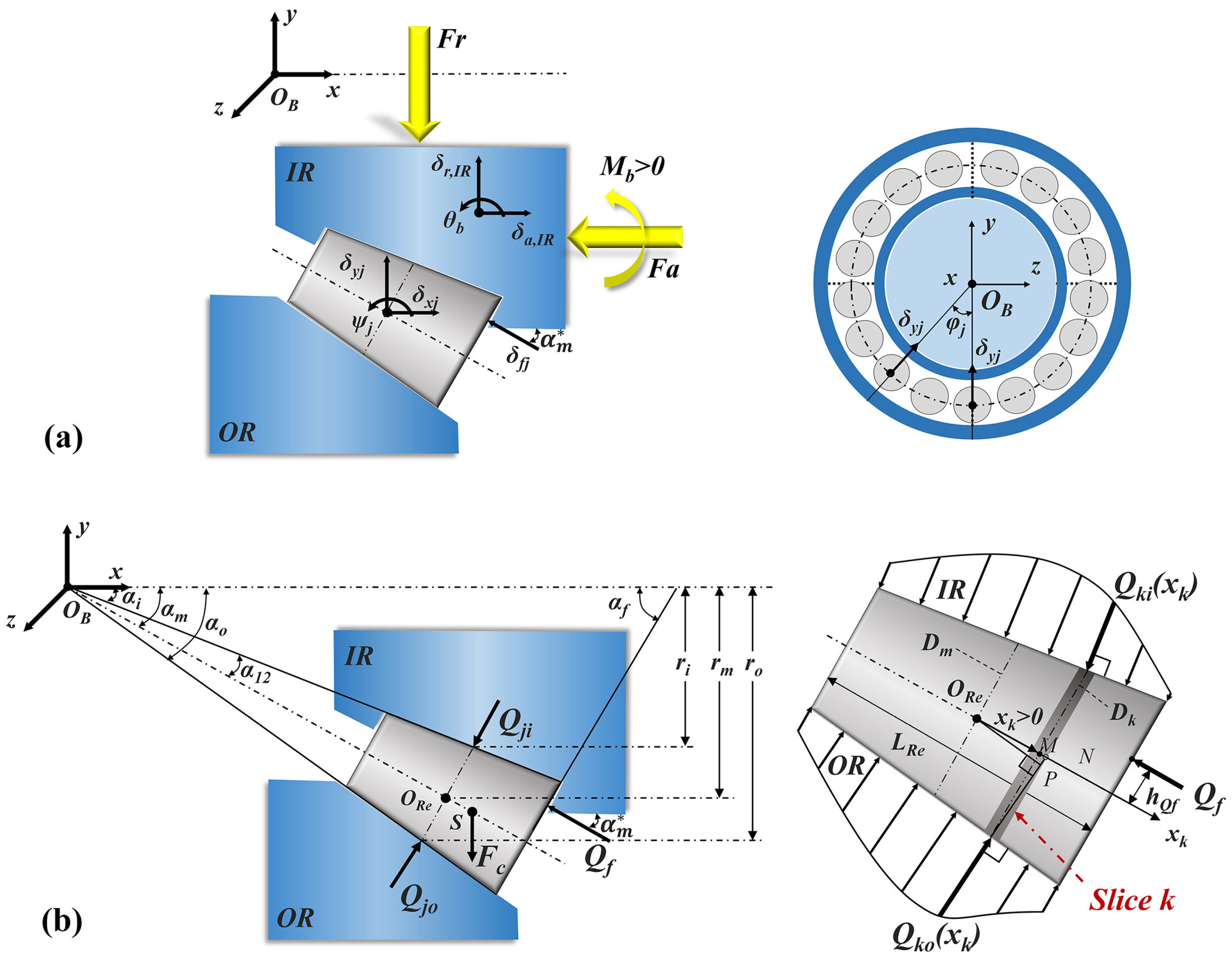
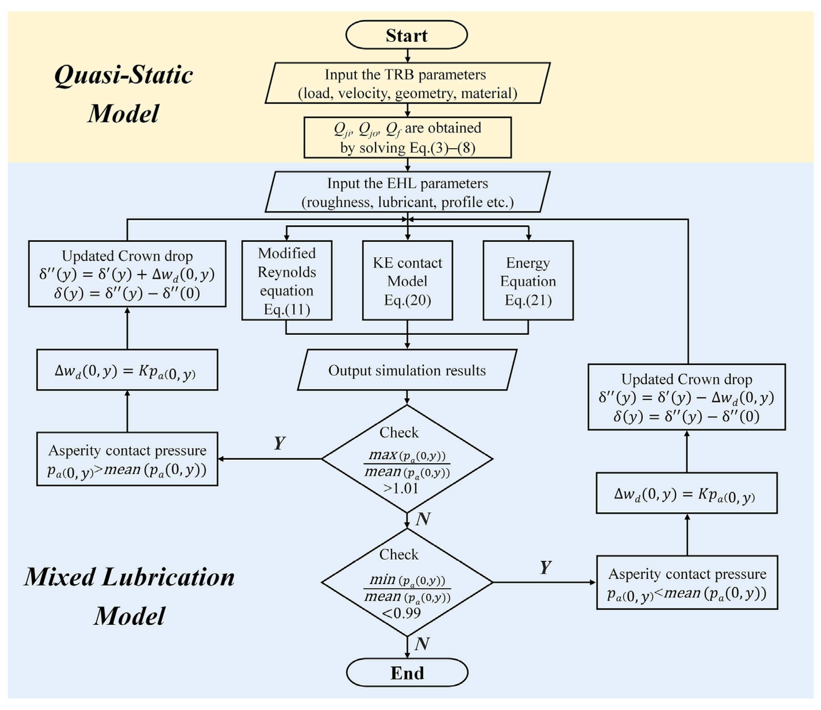
2.1. Quasi-Static Model of a Tapered Roller Bearing

Figure 1a shows the degrees of freedom (DOF) of a tapered roller bearing (TRB). The outer race (OR) is fixed in space with a center of O_B. The inner race (IR) has three DOFs; one of them is due to the bending moment M_b. Each rolling element (RE) has three DOFs as well. Thus, there are 3 + 3Z DOFs for computing the internal load distribution of the whole bearing, where Z is the number of rollers.

The geometry features and the normal loads on a single element are depicted in Figure 1b. Each roller is divided into n_s circular slices with the same thickness along the length L_Re. The resultant force Q_ji between the IR and the roller is the sum of normal loads acting on each slice.

$$Q_{ji}(j)={\displaystyle \sum _{k=1}^{n_s}{Q}_{ki}}(k,j)=\frac{C_L}{n_s}{\displaystyle \sum _{k=1}^{n_s}{\stackrel{⏜}{{\delta }_{ki}}}^{10/9}{f}_k}(k)$$

(1)

in which C_L is the contact stiffness coefficient for two-side deformation of the roller on the IR and OR, $\stackrel{⏜}{{\delta }_{ki}}$ is the modified deformation on slice k of the IR of the roller #j and f_k is Reusner’s correction factor of the load on slice k of the roller #j.

Similarly, the resultant force Q_jo between the OR and the roller can be written as

$$Q_{jo}(j)={\displaystyle \sum _{k=1}^{n_s}{Q}_{ko}}(k,j)=\frac{C_L}{n_s}{\displaystyle \sum _{k=1}^{n_s}{\stackrel{⏜}{{\delta }_{ko}}}^{10/9}{f}_k}(k)$$

(2)

in which $\stackrel{⏜}{{\delta }_{ko}}$ is the modified deformation on slice k of the OR of the roller #j.

In the y-direction, the radial load F_r acting on the bearing equals to sum of the forces Q_jo acting on the OR and all rollers. Therefore, the nonlinear force balance equation relating to the unknown DOFs of ${\delta }_{r,IR}$ is expressed as

$$F_r-\frac{C_L}{n_s}{\displaystyle \sum _{j=1}^Z{\displaystyle \sum _{k=1}^{n_s}{\stackrel{⏜}{{\delta }_{ko}}}^{10/9}{f}_k}(k)}\cos {\alpha }_o\cos {\phi }_j=0$$

(3)

where ${\alpha }_o$ is the outer race contact angle, and ${\phi }_j$ is the position angle of the roller #j.

Meanwhile, the axial load F_a acting on the bearing equals the sum of the forces Q_ji acting on the IR and all rollers in the x-direction. As a result, the nonlinear force balance equation relating to unknown DOFs ${\delta }_{a,IR}$ is given by

$$F_a-\frac{C_L}{n_s}{\displaystyle \sum _{j=1}^Z{\displaystyle \sum _{k=1}^{n_s}{\stackrel{⏜}{{\delta }_{ko}}}^{10/9}{f}_k}(k)}\sin {\alpha }_o=0$$

(4)

Each roller has a different bending moment $M_{bj}$. However, the sum of all moments $M_{bj}$ equals the given bending moment $M_b$ acting on the bearing in the direction z. Hence, the nonlinear moment balance equation relating to unknown DOFs ${\theta }_b$, which is a function of bending deformation ${\delta }_{kM}$, yields to

$$M_b-\frac{C_L{}^{\prime }}{n_s}{\displaystyle \sum _{j=1}^Z{\displaystyle \sum _{k=1}^{n_s}{l}_{kM}{\stackrel{⏜}{{\delta }_{kM}}}^{10/9}{f}_k}(k)}\cos {\phi }_j=0$$

(5)

where $C_L{}^{\prime }$ is the contact stiffness coefficient for one-side deformation at the rib contact regime, $l_{kM}$ is the moment arm, and $\stackrel{⏜}{{\delta }_{kM}}$ is the modified bending deformation on slice k.

Besides the above nonlinear equations relating to the three DOFs of IR, each roller also has three DOFs, ${\delta }_{yj}$, ${\delta }_{xj}$ and ${\psi }_j$, in the x, y, and z directions, respectively. Using the force balance equations of all rollers, two sets of Z nonlinear equations in the directions of x and y can be written as

$$-Q_{ji}\cos {\alpha }_i+Q_{jo}\cos {\alpha }_o+Q_f\sin {\alpha }_m^{\ast }-F_c=0$$

(6)

$$-Q_{ji}\sin {\alpha }_i+Q_{jo}\sin {\alpha }_o-Q_f\cos {\alpha }_m^{\ast }=0$$

(7)

where ${\alpha }_i$ is the inner race contact angle, ${\alpha }_m^{\ast }$ is the rib contact angle and F_c is the centrifugal force.

Similarly, when the moments of all rollers are balanced in the direction z, the set of Z nonlinear equations for the DOF ${\psi }_j$ are written as

$$\begin{array}{l}(-{\displaystyle \sum _{k=1}^{<n_{s,12}}{l}_{kL}{Q}_{ko}}+{\displaystyle \sum _{k\ge n_{s,12}}^{n_s}{l}_{kR}{Q}_{ko}})\cos {\phi }_j+({\displaystyle \sum _{k=1}^{<n_{s,12}}{l}_{kL}{Q}_{ki}}-{\displaystyle \sum _{k\ge n_{s,12}}^{n_s}{l}_{kR}{Q}_{ki}})\cos {\phi }_j-\\ F_c{l}_c\cos {\phi }_j+Q_f{h}_{Qf}\cos {\phi }_j+M_{bj}(j)=0\end{array}$$

(8)

in which $l_{kL}$ and $l_{kR}$ are the moment arms O_ReP shown in Figure 1b, n_s,12 equals (n_s + 1)/2, and l_c and h_Qf are the moment arm of the centrifugal force F_c and the rib force Q_f, respectively.

To sum up, a nonlinear equation system is derived by the 3 + 3Z equations written in Equations (3)–(8). The system describes a computational model that enables the calculation of the internal load distribution for a tapered roller bearing under given radial, axial and moment loads. The Levenberg and Marquardt method based on the Least Squares Method (LSM) was applied to solve the nonlinear equation system. More details of Equations (1)–(8) and the Levenberg and Marquardt method can be found in Reference [10].

2.2. Mixed Lubrication Model of Finite Line Contacts

After solving the normal forces acting on each roller in a TRB, a mixed lubrication model is needed to calculate the pressure, lubricant film thickness and temperature distributions within any roller/raceway contacts. Additionally, in the present study, TEHLs of finite line contacts are assumed under quasi-static and aligned conditions.

Taking a representative contact between a tapered roller and the IR for example, the governing equations for the mixed lubrication analysis are given as follows:

2.2.1. Velocity Relationship

Due to the contact angles of the TRB, the surface velocities in the contact area vary along the contact line. As shown in Figure 1b, the entrainment velocities of the roller–inner raceway can be expressed as

$$\overrightarrow{u_{ei}}=\frac{1}{2}\left[{\omega }_r\overrightarrow{r}+({\omega }_i-{\omega }_c)\overrightarrow{r_i}\right]$$

(9)

where $\overrightarrow{r}$ and $\overrightarrow{r_i}$ are the radii of the roller and the inner race, ${\omega }_r$ is the angular velocity of the roller around its axis, ${\omega }_i$ is the angular velocity of the inner race, and ${\omega }_c$ is the angular velocity of the roller rotating with respect to the $O_{B}x$ axis. Assuming the outer race control and the slide–roll ratio s, ${\omega }_c$ and ${\omega }_r$ are expressed as

$$\left\{\begin{array}{c}{\omega }_c=\frac{1}{2}\frac{2-s}{2r_m+sr}{\omega }_i{r}_i\\ {\omega }_r=\frac{r_o}{r}{\omega }_c=\frac{1}{2}\frac{2-s}{2r_m+sr}\frac{r_o{r}_i}{r}{\omega }_i\end{array}\right.$$

(10)

where r equals D_m/2, $r_i$, $r_m$ and $r_o$ are shown in Figure 1b, and s is the slide–roll ratio between the roller and the IR.

2.2.2. Reynolds Equation

Based on the work of Patir and Cheng [21,22], the average flow Reynolds equation for rough surfaces is given as

$$\frac{\partial }{\partial x}({\Phi }_x\frac{\rho h^3}{12\eta }\frac{\partial p_h}{\partial x})+\frac{\partial }{\partial y}({\Phi }_y\frac{\rho h^3}{12\eta }\frac{\partial p_h}{\partial y})=u_{ei}\frac{\partial (\rho h)}{\partial x}+u_{ei}s{R}_q\frac{\partial {\Phi }_s}{\partial x}$$

(11)

in which ${\Phi }_x$ and ${\Phi }_y$ are the flow factors in the x-direction and y-direction, $\rho$ and $\eta$ are the density and the viscosity of the lubricant, respectively, h is the nominal film thickness, $p_h$ is the hydrodynamic pressure, $R_q$ is the composite standard deviation of roughness and ${\Phi }_s$ is the shear flow factor. In solving Equation (11), the pressure boundary conditions are written as

$$p_h(x_{in},y)=p_h(x_{out},y)=p_h(x,y_{in})=p_h(x,y_{out})=0,\frac{\partial p_h(x_{out},y)}{\partial x}=0$$

2.2.3. Film Thickness Equation

For a finite line contact problem, the local lubricant film thickness h can be expressed as

$$h(x,y)=h_0+g(x,y)+v(x,y)$$

(12)

where $h_0$ represents the approach between the two bodies, and $g(x,y)$ is due to the original geometry profile that can be calculated by

$$g(x,y)=R_x(y)-\sqrt{\delta (y)-x^2}$$

(13)

in which $R_x(y)$ is the equivalent radius along the contact line and $\delta (y)$ is the crown drop relating to the roller profile.

$v(x,y)$ is the sum of elastic deformations of contacting surfaces due to pressure, calculated by the well-known Boussinesq integration:

$$v(x,y)=\frac{2}{\pi E^{\prime }}{\displaystyle {\iint }_{\Omega }\frac{p_t(x^{\prime },y^{\prime })}{\sqrt{{(x-x^{\prime })}^2+{(y-y^{\prime })}^2}}}d{x}^{\prime }d{y}^{\prime }$$

(14)

where $p_t$ is the sum of the hydrodynamic pressure $p_h$ and the asperity contact pressure $p_a$.

However, Boussinesq integration is under half-space assumption, which leads to incorrect pressure increases near free edges. A correction factor, $\psi$, proposed by Guilbault [36], was applied to correct the shear and normal stress influence on displacements through the mirroring process and can be approximated by the following formulation:

$$\psi =1.29-\frac{1}{1-\nu }(0.08-0.5\nu )$$

(15)

in which $\nu$ is the Poisson’s ratio.

2.2.4. Viscosity and Density Relationships

There are two types of lubricant in TRBs, either lubricating oils or greases. Grease consists of thickener and base oil, and its main advantages are ease in application and natural sealing ability. However, it is still difficult to model its rheological behavior under high shear rate, high pressure and non-constant temperature conditions precisely due to the complicated dynamics of its soap network in EHL contacts. Based on the experimental findings by Cen [37], the grease film thickness at EHL contacts can be calculated by using the base oil viscosity at higher entrainment velocities. Hence, the present study only considers base oil lubrication for the sake of simplicity.

In Equation (11), the oil lubrication viscosity is considered as a function of pressure and temperature, and one of the commonly used viscosity equations is the Roelands law [38]:

$$\eta (p_h,T)={\eta }_0\exp \left\{(\ln {\eta }_0+9.67)\left[-1+{(1+5.1\times {10}^{-9}{p}_h)}^Z(\frac{T-138}{T_0-138}){}^{-S0}\right]\right\}$$

(16)

The density is also assumed to be dependent on pressure and temperature, usually expressed as [39,40]

$$\rho (p_h,T)={\rho }_0\left[1+\frac{A{p}_h}{1+B{p}_h}+D(T-T_0)\right]$$

(17)

in which A, B and D are pressure–density coefficients. The parameters common to all results in this paper are: $A=0.6\times {10}^{-9} P{a}^{-1}$, $B=1.7\times {10}^{-9}{ \mathrm{Pa}}^{-1}$ and $D=-0.00065{ \mathrm{K}}^{-1}$.

In addition, oil lubrication usually behaves as a non-Newtonian fluid under high pressure and high shear rate. Hence, shear thinning should be considered in the TEHL calculation. Among several models of the shear thinning fluid behavior, the B-W model proposed by Bair and Winer [41] was used, written as

$$\dot{\gamma }=-\frac{{\tau }_{\lim }}{\eta (p_h,T)}\ln (1-\frac{\tau }{{\tau }_{\lim }})$$

(18)

where $\dot{\gamma }$ is the shear rate, $\tau$ is the shear stress and ${\tau }_{\lim }$ is the limiting shear stress, which can be illustrated as [42]

$${\tau }_{\lim }=({\tau }_{10}+{\gamma }_l{p}_h)exp({\beta }_l(\frac{1}{T}-\frac{1}{T_0}))$$

(19)

in which ${\tau }_{10}$ is the initial limiting shear stress, ${\gamma }_l$ is the pressure coefficient corresponding to maximum friction coefficient and ${\beta }_l$ is the temperature coefficient.

2.2.5. Asperity Contact Model

To calculate the asperity contact pressure under mixed lubrication, the stochastic rough surface contact model proposed by Kogut and Etsion (KE model) was used [23,24,25]. This model accounts for the elastic, first elastic–plastic, second elastic–plastic, and fully plastic deformation of asperities, and it can be written as

$$\begin{array}{l}{p}_a=\frac{2}{3}\pi {\beta }_{s}K{\omega }_c^{\ast }{H}_d({\displaystyle {\int }_{d^{\ast }}^{d^{\ast }+{\omega }_c^{\ast }}{I}^{1.5}+}1.03{\displaystyle {\int }_{d^{\ast }+{\omega }_c^{\ast }}^{d^{\ast }+6{\omega }_c^{\ast }}{I}^{1.425}+}1.4{\displaystyle {\int }_{d^{\ast }+6{\omega }_c^{\ast }}^{d^{\ast }+110{\omega }_c^{\ast }}{I}^{1.263}+}\frac{3}{K}{\displaystyle {\int }_{d^{\ast }+110{\omega }_c^{\ast }}^{\infty }{I}^1})\\ \left\{\begin{array}{c}{I}^b={(\frac{z^{\ast }-d^{\ast }}{{\omega }_c^{\ast }})}^b{\Phi }^{\ast }(z^{\ast })d{z}^{\ast },K=0.454+0.41\nu \\ {\omega }_c^{\ast }=\frac{{\omega }_c}{{\sigma }_0}=\frac{R_{as}}{{\sigma }_0}{(\frac{\pi K{H}_d}{E^{\prime }})}^2,d^{\ast }=h-\frac{1}{\sqrt{48}\pi {\beta }_s}\end{array}\right.\end{array}$$

(20)

where ${\beta }_s$ is the surface roughness parameter, which usually equals 0.05 [43], the hardness coefficient K is related to Poisson’s ratio of the softer material (see CEB friction model [44]), ${\omega }_c^{\ast }$ is the critical interference value of the elastic and the elastoplastic deformation regime, $R_{as}$ is the mean radius of asperity, $H_d$ is the hardness of the softer material, $z^{\ast }$ is the asperity height, ${\Phi }^{\ast }(z^{\ast })$ is the asperity heights probability density function which is assumed to be Gaussian and $d^{\ast }$ is the asperity separation. All the dimensionless values are normalized by the standard deviation of roughness ${\sigma }_0$ and denoted by *.

2.2.6. Thermal Effect

The calculation of 3D temperature distribution follows the energy equation within a mixed lubrication contact, which is given by

$$c\rho (u\frac{\partial T}{\partial x}+v\frac{\partial T}{\partial y}-w\frac{\partial T}{\partial z})=k\frac{{\partial }^{2}T}{\partial z^2}-\frac{T}{\rho }\frac{\partial \rho }{\partial T}(u\frac{\partial \rho }{\partial x}+v\frac{\partial \rho }{\partial y})+\eta \left[{\left(\frac{\partial u}{\partial z}\right)}^2+{\left(\frac{\partial v}{\partial z}\right)}^2\right]+{\tau }_a\sqrt{{\left(\frac{\partial u}{\partial z}\right)}^2+{\left(\frac{\partial v}{\partial z}\right)}^2}$$

(21)

where $c$ and $k$ are the specific heat and conductivity of the lubricant, respectively, the shear stress of the asperity contact ${\tau }_a$ equals ${\mu }_a{p}_a$ and ${\mu }_a$ is the friction coefficient of the asperity contact.

The boundary conditions for surface temperature are written as

$$\left\{\begin{array}{c}T(x,y,0)=\frac{k_1}{\sqrt{\pi {\rho }_1{c}_1{k}_1{u}_1}}{{\displaystyle {\int }_{-\infty }^x\left.\frac{\partial T}{\partial z}\right|}}_{x,y,0}\frac{ds}{\sqrt{x-s}}+T_0\\ T(x,y,h)=\frac{k_1}{\sqrt{\pi {\rho }_2{c}_2{k}_2{u}_2}}{{\displaystyle {\int }_{-\infty }^x\left.\frac{\partial T}{\partial z}\right|}}_{x,y,h}\frac{ds}{\sqrt{x-s}}+T_0\end{array}\right.$$

(22)

2.2.7. Load Balance

In mixed lubrication, an external normal load acting on the roller/IR contact is balanced by the hydrodynamic pressure and asperity contact pressure together as follows:

$$Q_{ji}={\displaystyle \underset{\Omega }{\iint }{p}_{h}dxdy}+{\displaystyle \underset{\Omega }{\iint }{p}_{a}dxdy}$$

(23)

where $Q_{ji}$ is the external normal load, and $\Omega$ means the contact region.

2.3. Numerical Running-In Method

Running-in is a traditional and conventional technique widely used in industry for the improvement of the conformity of sliding and rolling contacts of machine components at the microscale under appropriate mild conditions in the initial operation phase. After a proper running-in process, the surface topographical, physical and chemical structures, including profiles, surface roughness, compositions and microstructures, transform from their initial as-finished forms due to wear, tribochemical reactions and phase transformations occurred during running-in too in some conditions. Differing from conventional running-in, which is carried out in a real machine system in the operation stage, numerical running-in aims to achieve a similar effect on modifications of surface profile as that of a physical running-in by the means of computer simulations in the design stage of machine elements. The approach was proposed by authors and first applied to the modification of cylindrical roller profile [33]. In the present paper, the numerical running-in method is used in tapered roller bearings to seek the optimal design of a tapered roller profile.

As presented in Reference [33], the wear depth in each step of iterations can be determined with the aid of Archard’s wear law as follows:

$$\Delta w_d(x,y)=K_w\frac{p_a(x,y)\Delta S}{H_d}$$

(24)

where $\Delta w_d$ is the wear depth increment, $K_w$ is the wear coefficient, $\Delta S$ is the sliding distance increment and $H_d$ is the material hardness.

When $K_w$, $\Delta S$ and $H_d$ are constants, the wear depth increment is proportional to the asperity contact pressure. The optimized crown drop at position y is updated step-by-step, as shown below, until the calculated asperity contact pressure $p_a(0,y)$ meets a set convergence condition.

$${\delta }^{″}(y)={\delta }^{\prime }(y)+\Delta w_d(0,y)$$

(25)

in which ${\delta }^{\prime }(y)$ is the crown drop at position y in the previous step and ${\delta }^{″}(y)$ is the updated one.

The flowchart of the optimization process for the crowning profile is shown in Figure 2. At first, the internal load distribution in a TRB is calculated by using the quasi-static model described in Section 2.1 above. Then, the roller bearing the maximum load is focused on, and its pressure, lubricant film thickness and temperature distributions are analyzed with the mixed lubrication model in Section 2.2. The third step is to check the ratio of the maximum asperity contact pressure, $\max (p_a(0,y))$, to the mean asperity contact pressure, $\mathrm{mean}(p_a(0,y))$. If the ratio is greater than 1.01, Equations (24) and (25) are used to update the crown drop at that point. Meanwhile, the minimum contact pressure, $\min (p_a(0,y))$, is also compared with the mean asperity contact pressure, $\mathrm{mean}(p_a(0,y))$, and if it is less than the mean value, a negative crown drop is applied. Finally, a profile with uniform asperity contact pressure can be obtained, which is the optimal crowning profile.

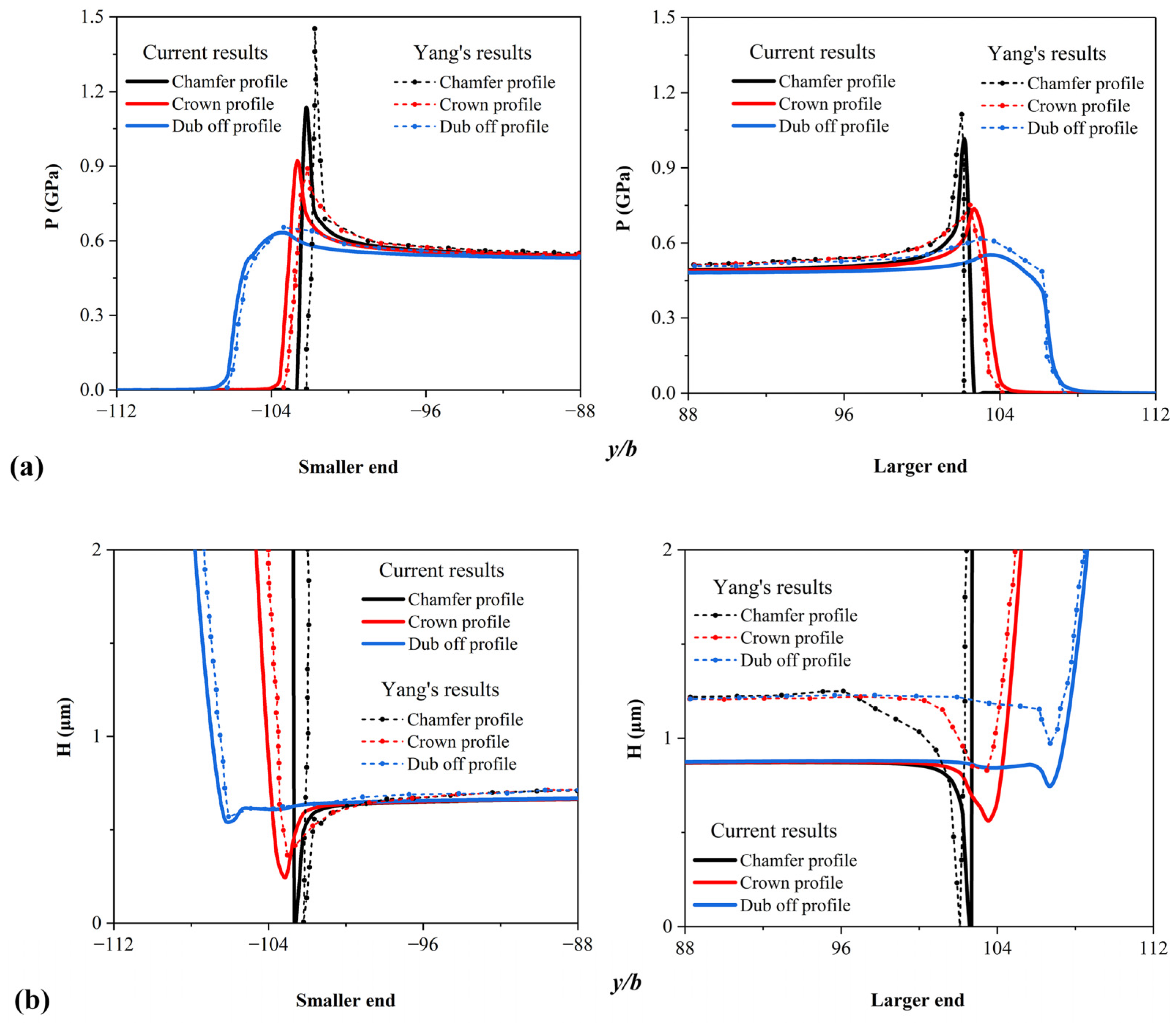
3. Numerical Model Validation

In Reference [34], Yang calculated the distributions of the EHL pressure and lubricant film thickness for three tapered rollers with different profiles rolling on an infinite plane based on the following dimensionless input parameters: $\overline{W }{=3 \times 10}^{-5}, \overline{U }{=2 \times 10}^{-11}$.

To validate the mixed lubrication model used in the study, numerical EHL simulations were performed with the same values of input parameters (shown in

Table 1. Input parameters for the analyzed cases [34].

Parameter	Value	Parameter	Value
Half length of rollers, l, mm	20	Effective elastic modulus, $E^{\prime }$, GPa	228
Radius of rollers on the section y = 0, r, m	0.02	Material parameter, G, dimensionless	5000
Deflective angles of tapered rollers, $\beta$, (°)	10	Nominal maximum Hertzian pressure, $P_H$, GPa	0.5
Ambient viscosity of lubricant, ${\eta }_0$, Ns/m2	0.08	Angular velocities of rollers, ${\omega }_a$, rad/s	9.86
Ambient density of lubricant, ${\rho }_0$, kg/m3	870	Angular velocities of plane, ${\omega }_b$, rad/s	56.4

) as those in Reference [30]. As shown in Figure 3, the simulation results of the present study (denoted as current results in the figure) and Yang’s results are generally in good agreement, except that the calculated lubricant film thickness is slightly smaller. The discrepancy is attributed to the thermal effect described in the present study (the main thermal parameters are listed in

Table 2. Parameters of the thermal effect of current model.

Parameter	Value
Ambient temperature, $T_0$, K	313
Specific heat of lubricant, c, J/kg K	1880
Specific heat of solids, c1 and c2, J/kg K	460
Thermal conductivity of lubricant, k, W/m K	0.145
Thermal conductivity of solids, k1 and k2, W/m K	46
Density of the solids, ${\rho }_{\mathrm{a}}$ and ${\rho }_{\mathrm{b}}$, kg/m3	7850
Thermos-viscosity index, $\beta$, K−1	0.0585

), while the EHL analysis in Reference [30] was isothermal. We can see that both pressure and film thickness distributions are asymmetric, owing to the difference in size between the bigger and smaller ends of the tapered rollers, and that the crown and dub-off profiles give rise to more uniform distributions of lubricant film thickness and pressure near the ends than the chamfer profile.

4. Results and Discussion

4.1. Calculation Parameters of the Axial Box TRBs

TRBs are generally used in the axial boxes of trains on high-speed railways. Typical operation conditions of axial-box TRBs are listed in

Table 3. Main parameters of the TRB used in high-speed railway.

Parameter	Value	Parameter	Value
Constant axial load, $F_a$, KN	15	Length of rollers, $L_{Re}$, mm	50
Varying radial load, $F_r$, KN	10–50	Radius of rollers on the section y = 0, r, mm	13
Bearing rotation speed, N, 103 rpm	1–3	Mean pitch radius of bearing, $r_m$, mm	92.5
Bending moment, $M_b$, Nm	50	Outer race contact angle, ${\alpha }_o$, (°)	12
Number of bearing rollers, $Z$	17	Inner race contact angle, ${\alpha }_i$, (°)	9
Bearing diametric clearance, $P_d$, $\mathsf{\mu }\mathrm{m}$	30	Ambient temperature, $T_0$, K	353
Effective elastic modulus, $E^{\prime }$, GPa	226	Ambient viscosity of lubricant, ${\eta }_0$, Ns/m2	0.014
Poisson’s $\upsilon$ ratio,	0.3	Composite standard deviation of roughness, Rq, $\mathsf{\mu }\mathrm{m}$	0.5
Slide–roll ratio, s	0.05	Hardness of the softer material, Hd, GPa	4.04
Material parameter, G, dimensionless	4241	Mean radius of asperity, Ras, $\mathsf{\mu }\mathrm{m}$	10

. The thermal parameters are the same as in Table 2, and the bearing rotation speeds corresponding to the steady running speeds of the high-speed railway are shown in

Table 4. The relationship between the bearing rotation speed and the high-speed railway speed.

The Bearing Rotation Speed	The High-Speed Railway Speed
1000 rpm	152 km/h
1500 rpm	228 km/h
2000 rpm	304 km/h
2500 rpm	380 km/h
3000 rpm	456 km/h

.

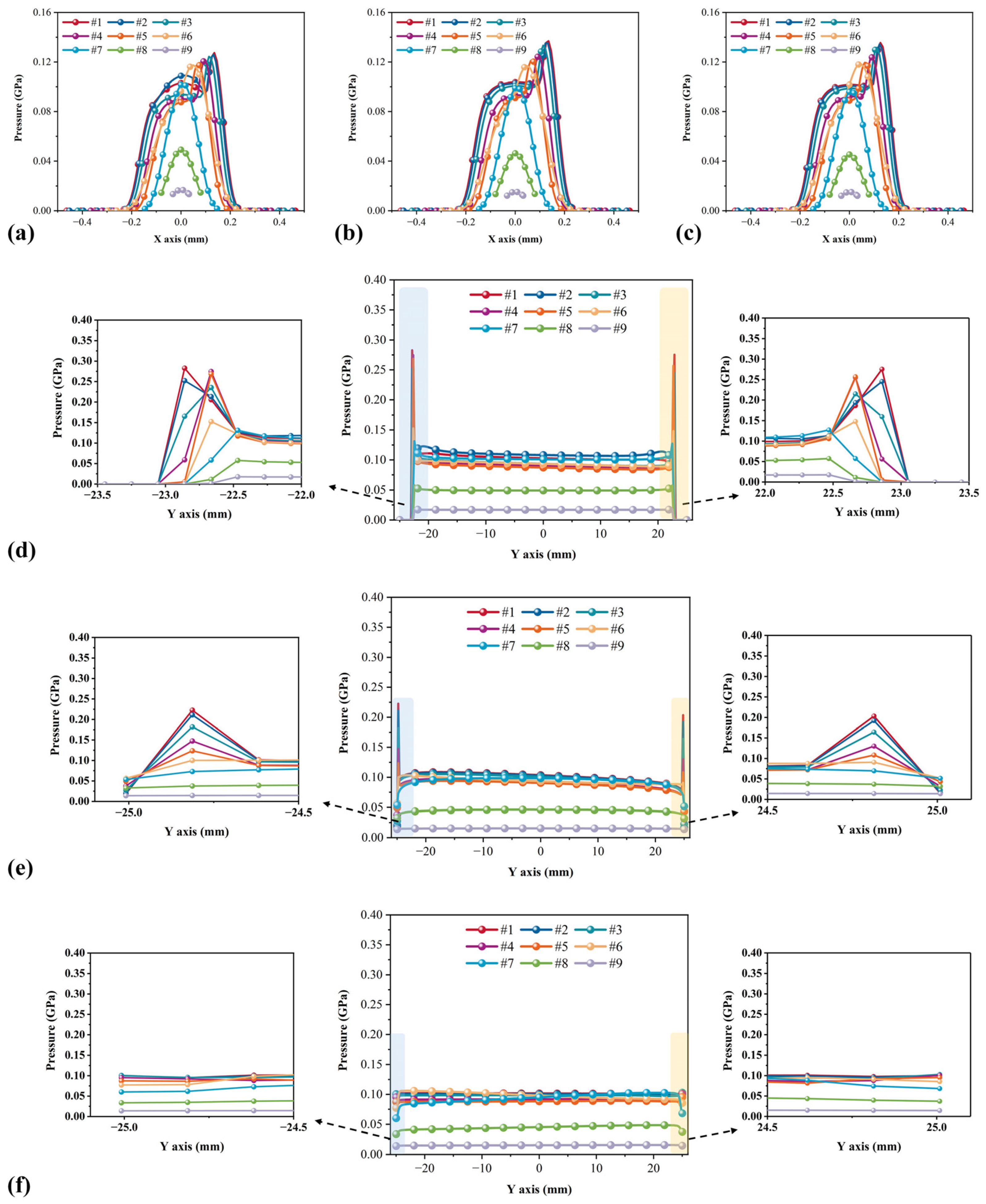
4.2. Internal Load Distributions

Figure 4 shows the calculated results of contact loads acting on each roller (half of rollers numbered as No.1 to No.9 are displayed for the sake of symmetry) under different radial loads and bearing rotation speeds. As the radial load increases, the rollers at the bottom bear higher loads no matter whether they contact with the inner or outer race. In contrast, the rollers at the top bear lighter loads. A minor difference in contact load between the inner and the outer raceways is caused by the centrifugal force F_c. As the bearing rotation speed increases, no significant change happens in internal load distributions, but huge differences in the TEHL results appear as well as the roller profile modifications, which are discussed later.

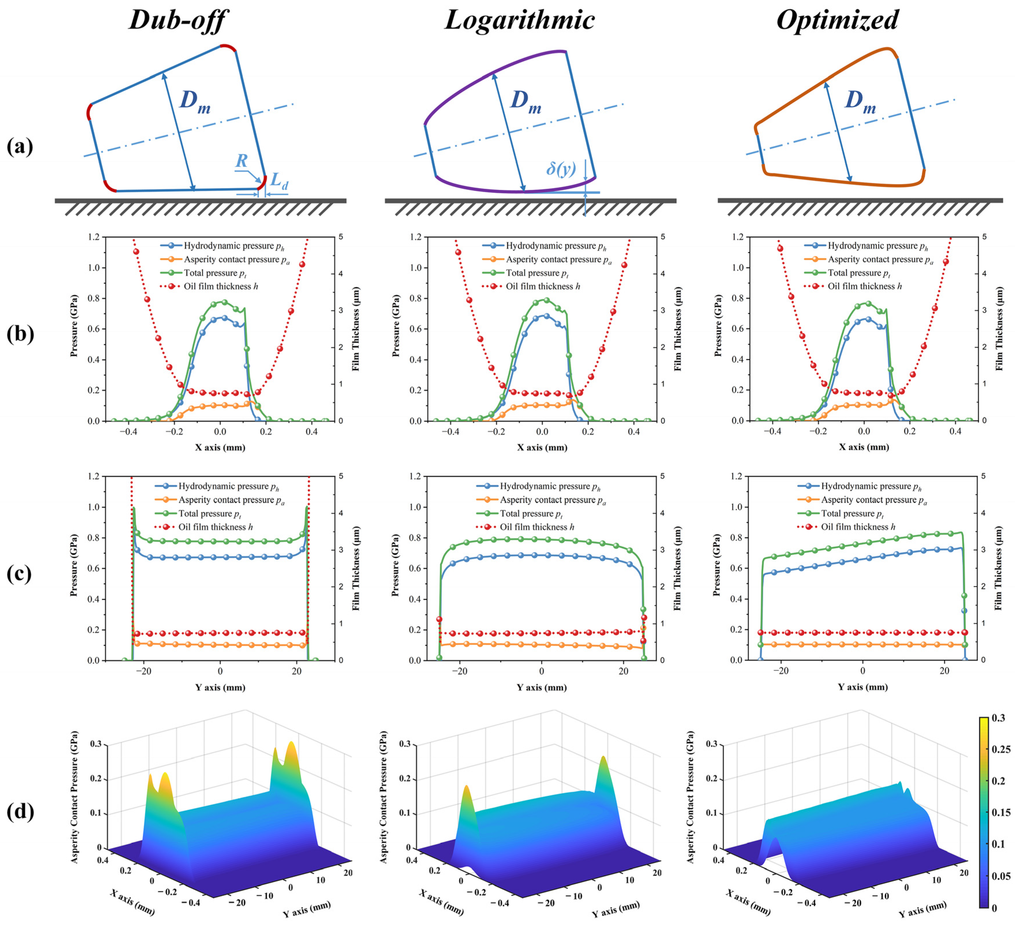
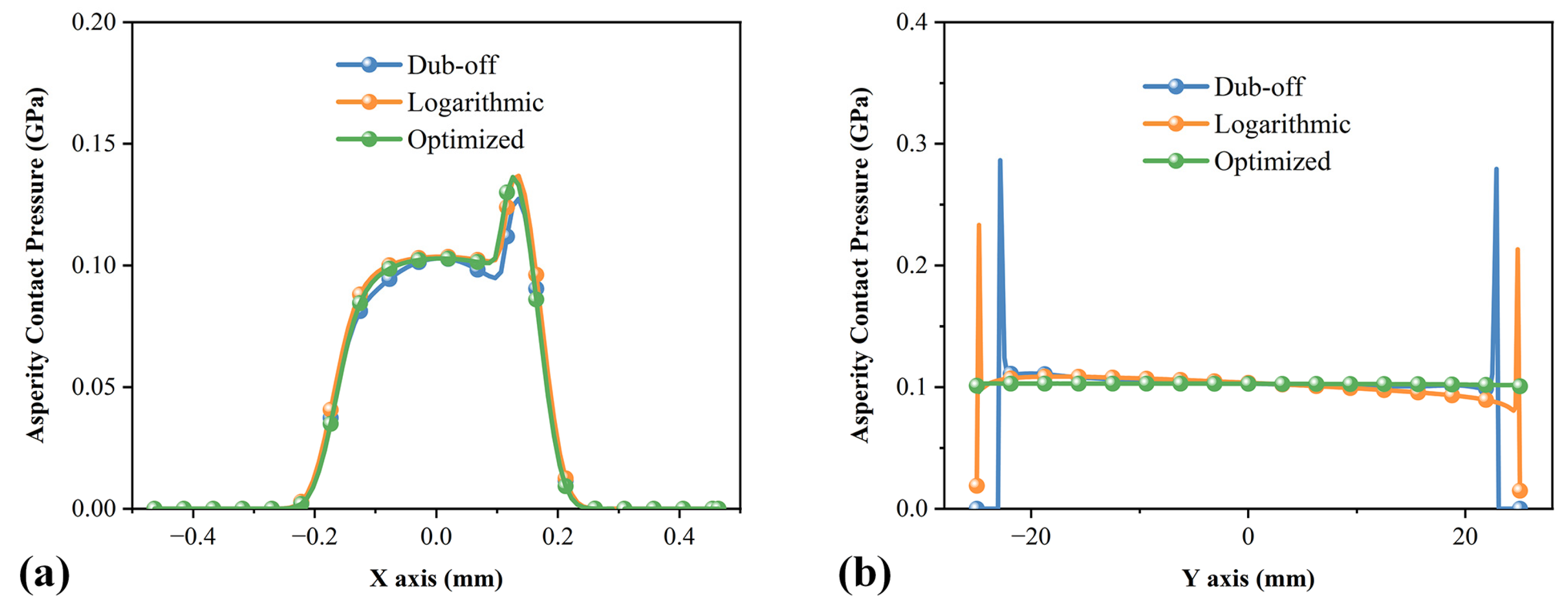
4.3. Effect of Different Axial Roller Profiles

In this section, the simulation results of the mixed lubrication of roller No.1 on the inner raceway—which is under the heaviest load among the all rollers—at typical working conditions ($F_a=15 \mathrm{KN}, F_r=40 \mathrm{KN}, N=2000 \mathrm{rpm}$) are presented, and the effect of roller profiles is demonstrated with three different forms: dub-off, logarithmic and running-in optimized profiles.

Figure 5a shows the diagrams of different roller profiles. For the roller with a dub-off profile, a rounding radius R is set as 30 mm and the rounding width L_d as 2.5 mm. The logarithmic profile is well-known for its uniformity of pressure distribution under static line contact conditions. It was proposed by Lundberg [26] and improved by Johns and Gohar [27], which can be expressed as a function

$$\delta (y)=\frac{W_r}{\pi LE{}^{\prime }}\ln \frac{1}{1-(1-0.6066b/L){(2y/L)}^2}$$

(26)

where $W_r$ is the load acting on the roller and the inner raceway, $L$ is the contact length, and $b$ is the half width of the nominal Hertzian line contact.

As shown in Figure 5b, there are no obvious differences between the three axial profiles along the rolling direction (y = 0). The maximum total pressure is about 0.7 GPa and close to the maximum Hertzian contact pressure. However, Figure 5c,d indicate that the differences in contact pressure are huge along the axial direction (x = 0). For the dub-off profile, no matter whether the pressure is hydrodynamic or asperity, it increases sharply at the edges. The maximum total pressure is about 0.9 Gpa, which is larger than the maximum Hertzian contact pressure. Though the hydrodynamic pressure does not rise sharply near the end with the logarithmic profile, the asperity contact pressure still has an obvious spike, which would result in severe local wear. Starting from the initial logarithmic profile, the axial profile was modified step by step by using the numerical running-in method described in Section 2.3. The comparison is shown in Figure 6. Obviously, for the profile after running-in (denoted as the optimized profile in the figure), the spikes of asperity contact pressure in the vicinity of the roller ends are eliminated, resulting in a much more uniform asperity contact pressure distribution in the axial direction.

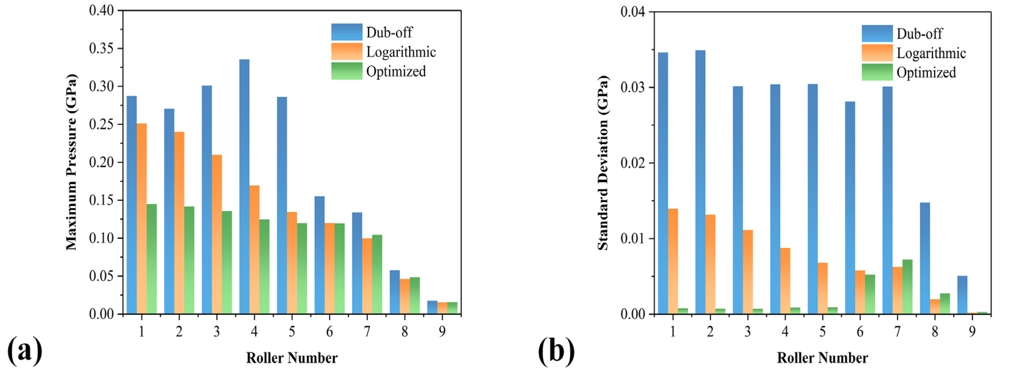
4.4. Influences on Bearing Performance

To reveal the effect of profiles on bearing performance, all rollers in a TRB are assumed to be crowned in the same axial profile as roller No.1 with either dub-off, logarithmic or running-in optimized profiles, and the mixed lubrication of all rollers in a TRB was analyzed, respectively.

The asperity contact pressure distributions of each roller along the rolling direction are presented in Figure 7a–c. Like roller No.1 discussed in Section 4.3, the asperity contact pressure distributions of the other rollers have no obvious difference, although the profiles change. It should be noted that from roller No.1 to No.9, the contact load decreases, and hence, the contact half-width becomes smaller and asperity contact pressure becomes lower, which means that the lubrication state of the rollers changes from mixed lubrication to full-film lubrication.

Figure 7d–f display the distributions along the axial direction of the rollers. For the bearing of rollers with the dub-off profile, only the rollers with light loads have no contact pressure spikes near the ends, and the asperity contact pressures of the other rollers are non-uniform. Compared with the dub-off profile, the logarithmic profile gives rise to lower edge contact pressure, but most of the rollers still have non-uniform contact pressure. Because of the deflective angles of tapered rollers, the entrainment velocities along the axial direction are different, and the pressures near the smaller ends are slightly higher than those at the larger end. In contrast to the profiles mentioned above, it is demonstrated that the profile modified by the running-in method is beneficial to reducing the end effect of stress concentration for all of the rollers, not just for roller No.1.

In addition, we also compared the maximum asperity contact pressures and standard deviations of the contact pressure of all rollers among the three profiles. As shown in Figure 8, it is clear that the optimized profile is advantageous in both aspects over the other ones, especially in respect to the standard deviations, which means that the asperity contact pressure distributions are smoother. However, the effect of the optimized profile for roller Nos. 7 and 8 is worse than that of the logarithmic profile. The differences between the two types of profiles are small and ignorable because the loads acting on the two rollers are relatively light.

4.5. Effects of Other Factors on Asperity Contact Pressure Distributions

4.5.1. Radial Load (Fr) Effect

The radial load has a critical influence on mixed lubrication and asperity contact pressure distributions. Figure 9a indicates that the roller bearing under heavier loads needs larger crown drops at the smaller ends. Figure 9b–d compare the pressure distributions of the three profiles under different radial loads $Fr=10 \mathrm{KN}, 30 \mathrm{KN}, 50 \mathrm{KN}$. The contact pressures near the ends become higher as the radial load increases. In all cases, the optimized profile shows the best performance and effectively reduces the end effect.

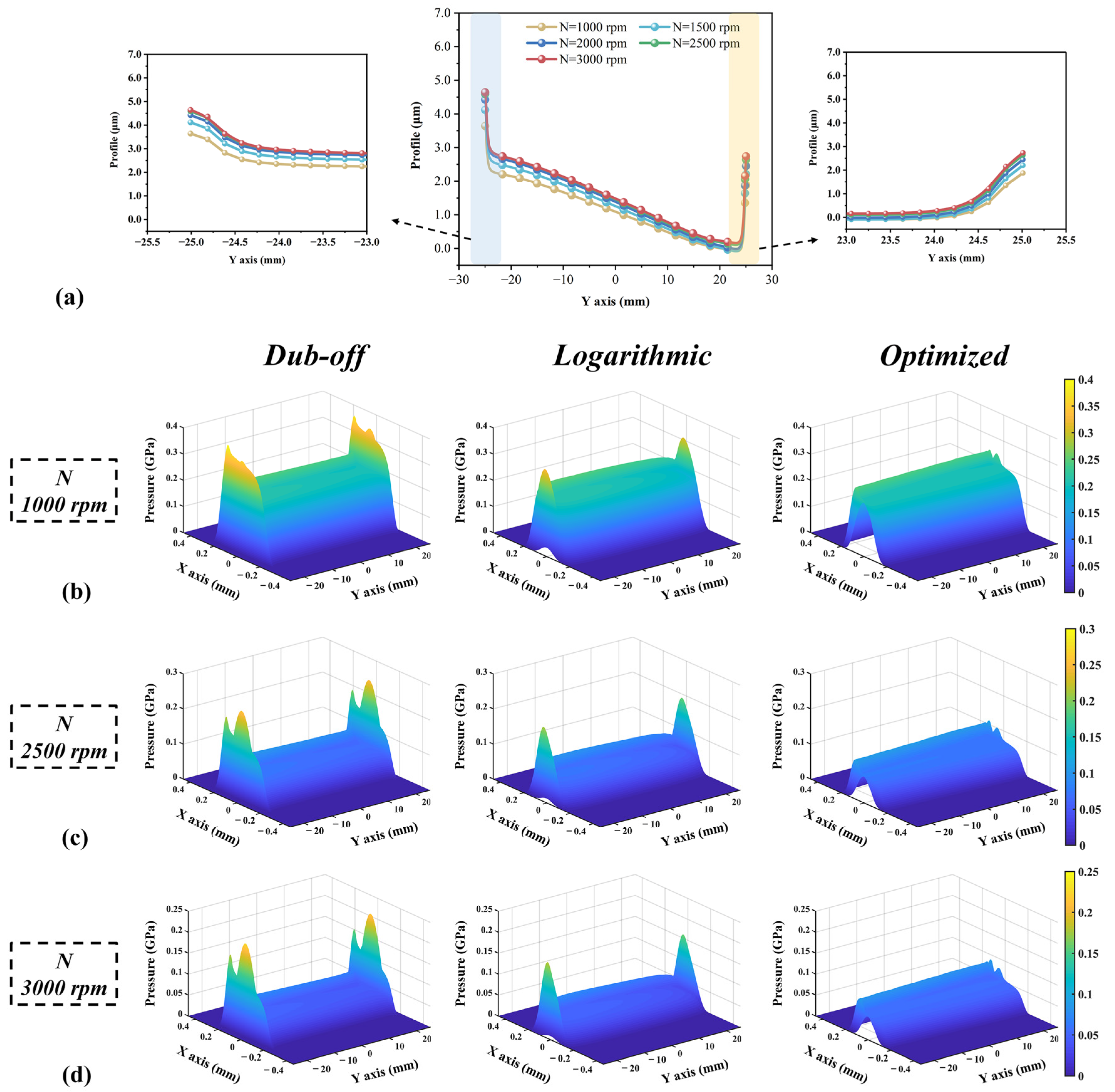
4.5.2. Rotation Speed (N) Effect

In addition to the radial load, the rotation speed is also an important factor in determining the lubrication state. As discussed in Section 4.2, the increase in rotation speed has little influence on load distribution but has a great effect on the modified profile and TEHL performance, as shown in Figure 10. We can see that the higher the speed is, the larger the crown drop and the lower the contact pressure. Obviously, the optimized profile is better than the other profiles in terms of asperity contact pressure uniformity.

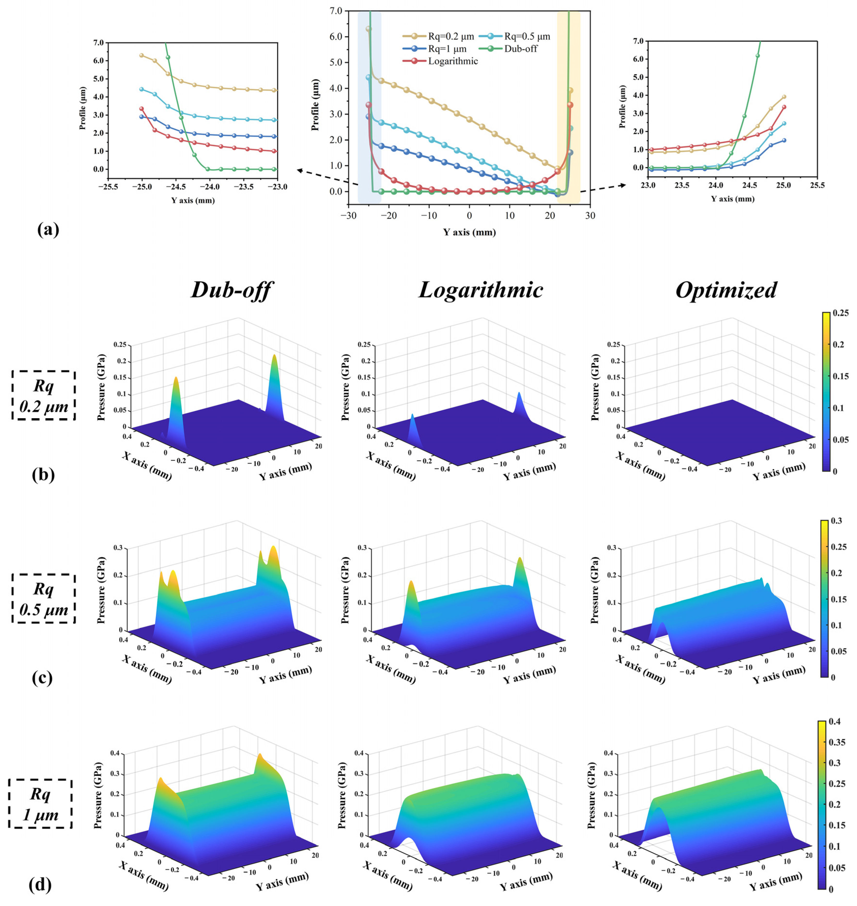
4.5.3. Standard Deviation of Roughness (Rq) Effect

The optimized profiles are related to standard deviations of roughness, as shown in Figure 11a. When Rq equals $0.2 \mathsf{\mu }\mathrm{m}$, non-uniform contact pressure only appears at the ends of the roller. It can be also found that with a smaller Rq, a larger crown drop is needed to achieve smoother pressure distributions. Moreover, due to the asymmetry of the tapered roller, the smaller end needs a larger amount of modification than the larger end. It is interesting to note that for the larger end (profile < 0), padding is needed instead of trimming to achieve a smooth asperity contact pressure distribution, as shown in Figure 11b–d.

5. Conclusions

For the purposes of making the asperity contact pressure of tapered rollers uniform and reducing the sharp spikes of the contact pressure in the vicinity of the roller ends, a numerical running-in method is applied, and a new asymmetric optimized profile is found.

Compared with the traditional profiles, it is clear that the optimized profile has immense advantages in terms of the asperity contact pressure uniformity and the elimination of the end effect of stress concentration not only for a single tapered roller but also for all tapered roller bearings. The numerical running-in method is proved to be suitable for various working conditions, and the optimized roller profile always shows better performance and effectively reduces the end effect. It is hoped that this method will be helpful in the improvement of tapered roller bearing design in the bearing industry.

References

1. Hong, S.-W.; Tong, V.-C. Rolling-element bearing modeling: A review. Int. J. Precis. Eng. Manuf. 2016, 17, 1729–1749. [Google Scholar] [CrossRef]
2. Cao, H.; Niu, L.; Xi, S.; Chen, X. Mechanical model development of rolling bearing-rotor systems: A review. Mech. Syst. Signal Process. 2018, 102, 37–58. [Google Scholar] [CrossRef]
3. Stacke, L.-E.; Fritzson, D.; Nordling, P. BEAST—A rolling bearing simulation tool. Proc. Inst. Mech. Eng. Part K J. Multi-body Dyn. 1999, 213, 63–71. [Google Scholar] [CrossRef]
4. Rahnejat, H.; Gohar, R. Design of profiled taper roller bearings. Tribol. Int. 1979, 12, 269–275. [Google Scholar] [CrossRef]
5. Creju, S.; Bercea, I.; Mitu, N. A dynamic analysis of tapered roller bearing under fully flooded conditions part 1: Theoretical formulation. Wear 1995, 188, 1–10. [Google Scholar] [CrossRef]
6. Creţu, S.; Mitu, N.; Bercea, I. A dynamic analysis of tapered roller bearings under fully flooded conditions part 2: Results. Wear 1995, 188, 11–18. [Google Scholar] [CrossRef]
7. Yamashita, R.; Dowson, D.; Taylor, C.M. An Analysis of Elastohydrodynamic Film Thickness in Tapered Roller Bearings. Tribol. Ser. 1997, 32, 617–637. [Google Scholar] [CrossRef]
8. Zheng, J.; Ji, J.; Yin, S.; Tong, V.-C. Internal loads and contact pressure distributions on the main shaft bearing in a modern gearless wind turbine. Tribol. Int. 2020, 141, 105960. [Google Scholar] [CrossRef]
9. Zhang, C.; Gu, L.; Mao, Y.; Wang, L. Modeling the frictional torque of a dry-lubricated tapered roller bearing considering the roller skewing. Friction 2019, 7, 551–563. [Google Scholar] [CrossRef] [Green Version]
10. Nguyen-Schäfer, H. Computational Tapered and Cylinder Roller Bearings; Springer: Cham, Switzerland, 2019. [Google Scholar] [CrossRef]
11. Petrusevich, A.I. Fundamental conclusions from the contact-hydrodynamic theory of lubrication. Izv. Akad. Nauk SSSR 1951, 2, 209–233. [Google Scholar]
12. Dowson, D.; Higginson, G.R. A Numerical Solution to the Elasto-Hydrodynamic Problem. J. Mech. Eng. Sci. 1959, 1, 6–15. [Google Scholar] [CrossRef]
13. Gohar, R.; Cameron, A. The Mapping of Elastohydrodynamic Contacts. A S L E Trans. 1967, 10, 215–225. [Google Scholar] [CrossRef]
14. Wymer, D.G.; Cameron, A. Elastohydrodynamic lubrication of a line contact. Proc. Inst. Mech. Eng. 1974, 188, 221–238. [Google Scholar] [CrossRef]
15. Bahadoran, H.; Gohar, R. Oil Film Thickness in Lightly-Loaded Roller Bearings. J. Mech. Eng. Sci. 1974, 16, 386–390. [Google Scholar] [CrossRef]
16. Kushwaha, M.; Rahnejat, H.; Gohar, R. Aligned and misaligned contacts of rollers to races in elastohydrodynamic finite line conjunctions. Proc. Inst. Mech. Eng. Part C J. Mech. Eng. Sci. 2002, 216, 1051–1070. [Google Scholar] [CrossRef] [Green Version]
17. Kushwaha, M.; Rahnejat, H. Transient concentrated finite line roller-to-race contact under combined entraining, tilting and squeeze film motions. J. Phys. D: Appl. Phys. 2004, 37, 2018–2034. [Google Scholar] [CrossRef]
18. Liu, X.; Yang, P. Analysis of the thermal elastohydrodynamic lubrication of a finite line contact. Tribol. Int. 2002, 35, 137–144. [Google Scholar] [CrossRef]
19. Yang, P.; Yang, P. Analysis on the thermal elastohydrodynamic lubrication of tapered rollers in opposite orientation. Tribol. Int. 2007, 40, 1627–1637. [Google Scholar] [CrossRef]
20. Zhu, N.; Wang, J.; Ren, N.; Wang, Q.J. Mixed Elastohydrodynamic Lubrication in Finite Roller Contacts Involving Realistic Geometry and Surface Roughness. J. Tribol. 2012, 134, 011504. [Google Scholar] [CrossRef]
21. Patir, N.; Cheng, H.S. An Average Flow Model for Determining Effects of Three-Dimensional Roughness on Partial Hydrodynamic Lubrication. J. Lubr. Technol. 1978, 100, 12–17. [Google Scholar] [CrossRef]
22. Patir, N.; Cheng, H.S. Application of Average Flow Model to Lubrication Between Rough Sliding Surfaces. J. Lubr. Technol. 1979, 101, 220–229. [Google Scholar] [CrossRef]
23. Kogut, L.; Etsion, I. Elastic-Plastic Contact Analysis of a Sphere and a Rigid Flat. J. Appl. Mech. 2002, 69, 657–662. [Google Scholar] [CrossRef] [Green Version]
24. Kogut, L.; Etsion, I. A Finite Element Based Elastic-Plastic Model for the Contact of Rough Surfaces. Tribol. Trans. 2003, 46, 383–390. [Google Scholar] [CrossRef]
25. Kogut, L.; Etsion, I. A Static Friction Model for Elastic-Plastic Contacting Rough Surfaces. J. Tribol. 2004, 126, 34–40. [Google Scholar] [CrossRef] [Green Version]
26. Lundberg, G. Elastische Berührung zweier Halbräume. Forsch. Im Ingenieurwesen 1939, 10, 201–211. [Google Scholar] [CrossRef]
27. Johns, P.; Gohar, R. Roller bearings under radial and eccentric loads. Tribol. Int. 1981, 14, 131–136. [Google Scholar] [CrossRef]
28. Fujiwara, H.; Kawase, T. Logarithmic Profile of Rollers in Roller Bearing and Optimization of the Profile. Trans. Jpn. Soc. Mech. Eng. Ser. C 2006, 72, 3022–3029. [Google Scholar] [CrossRef] [Green Version]
29. Fujiwara, H.; Kobayashi, T.; Kawase, T.; Yamauchi, K. Optimized Logarithmic Roller Crowning Design of Cylindrical Roller Bearings and Its Experimental Demonstration. Tribol. Trans. 2010, 53, 909–916. [Google Scholar] [CrossRef]
30. Cui, L.; He, Y. A new logarithmic profile model and optimization design of cylindrical roller bearing. Ind. Lubr. Tribol. 2015, 67, 498–508. [Google Scholar] [CrossRef]
31. Poplawski, J.V.; Peters, S.M.; Zaretsky, E.V. Effect of Roller Profile On Cylindrical Roller Bearing Life Prediction—Part II Comparison of Roller Profiles. Tribol. Trans. 2001, 44, 417–427. [Google Scholar] [CrossRef]
32. Najjari, M.; Guilbault, R. Edge contact effect on thermal elastohydrodynamic lubrication of finite contact lines. Tribol. Int. 2014, 71, 50–61. [Google Scholar] [CrossRef]
33. Zhang, Y.; Cao, H.; Kovalev, A.; Meng, Y. Numerical Running-In Method for Modifying Cylindrical Roller Profile Under Mixed Lubrication of Finite Line Contacts. J. Tribol. 2019, 141, 041401. [Google Scholar] [CrossRef]
34. Yang, P.; Yang, P.; Liu, X. Numerical Analysis of Isothermal EHL for Tapered Roller. Tribology 2005, 25, 456–460. [Google Scholar]
35. Chen, F.; Wang, J.; Zhang, G. Elastohydrodynamic lubrication of tapered roller with logarithmic profile. Chin. J. Mech. Eng. 2011, 47, 143–148. [Google Scholar] [CrossRef]
36. Guilbault, R. A Fast Correction for Elastic Quarter-Space Applied to 3D Modeling of Edge Contact Problems. J. Tribol. 2011, 133, 031402. [Google Scholar] [CrossRef]
37. Cen, H.; Lugt, P.; Morales-Espejel, G.E. On the Film Thickness of Grease-Lubricated Contacts at Low Speeds. Tribol. Trans. 2014, 57, 668–678. [Google Scholar] [CrossRef]
38. Roelands, C.J.A.; Winer, W.O.; Wright, W.A. Correlational Aspects of the Viscosity-Temperature-Pressure Relationship of Lubricating Oils (Dr In dissertation at Technical University of Delft, 1966). J. Lubr. Technol. 1971, 93, 209–210. [Google Scholar] [CrossRef] [Green Version]
39. Zhu, N.; Wen, S.-Z. A Full Numerical Solution for the Thermoelastohydrodynamic Problem in Elliptical Contacts. J. Tribol. 1984, 106, 246–254. [Google Scholar] [CrossRef]
40. Peiran, Y.; Shizhu, W. A Generalized Reynolds Equation for Non-Newtonian Thermal Elastohydrodynamic Lubrication. J. Tribol. 1990, 112, 631–636. [Google Scholar] [CrossRef]
41. Bair, S.; Winer, W.O. A rheological model for elastohydrodynamic contacts based on primary laboratory data. J. Lubr. Technol. 1979, 101, 258–265. [Google Scholar] [CrossRef]
42. Houpert, L.; Flamand, L.; Berthe, D. Rheological and Thermal Effects in Lubricated E.H.D. Contacts. J. Lubr. Technol. 1981, 103, 526–532. [Google Scholar] [CrossRef]
43. Masjedi, M.; Khonsari, M.M. Film Thickness and Asperity Load Formulas for Line-Contact Elastohydrodynamic Lubrication with Provision for Surface Roughness. J. Tribol. 2012, 134, 011503. [Google Scholar] [CrossRef]
44. Chang, W.-R.; Etsion, I.; Bogy, D.B. Static Friction Coefficient Model for Metallic Rough Surfaces. J. Tribol. 1988, 110, 57–63. [Google Scholar] [CrossRef]
Figure 1. Description of the tapered roller bearing: (a) the degrees of freedom (DOF); and (b) the geometry features and the normal loads on a single element.
Lubricants 11 00097 g001
Figure 2. The flowchart of the running-in optimization of roller profile in TRB.
Lubricants 11 00097 g002
Figure 3. Comparison of current results and Yang’s results [34]: (a) pressure distributions and (b) film thickness distributions.
Lubricants 11 00097 g003
Figure 4. Contact loads between each component with varying radial loads and bearing rotation speeds: (a) description of roller number; (b) inner raceway contact load; (c) outer raceway contact load; and (d) rib contact load.
Lubricants 11 00097 g004
Figure 5. Pressure distributions and oil film thicknesses with different axial roller profiles under W = 7 . 513   ×   10 5 ,   U = 5 . 367   ×   10 11 ,   P H = 0 . 78   GPa : (a) diagrams of different roller profiles; (b) rolling direction, y = 0; (c) axial direction, x = 0; and (d) 3D images of asperity contact pressure.
Lubricants 11 00097 g005
Figure 6. Asperity contact pressure distributions with different axial roller profiles: (a) rolling direction, y = 0; and (b) axial direction, x = 0.
Lubricants 11 00097 g006
Figure 7. Asperity contact pressure distributions of each roller: (a) dub-off, rolling direction; (b) logarithmic, rolling direction; (c) optimized, rolling direction; (d) dub-off, axial direction; (e) logarithmic, axial direction; and (f) optimized, axial direction.
Lubricants 11 00097 g007
Figure 8. Comparisons of asperity contact pressure distributions of each roller: (a) maximum contact pressure and (b) standard deviation of contact pressure on the section of x = 0.
Lubricants 11 00097 g008
Figure 9. The effect of the radial load (Fr) under N = 2000 rpm, R q = 0.5   μ m : (a) The comparison of the profiles with different Fr; (b) contact pressures under F r = 10   KN ; (c) contact pressures under F r = 30   KN ; and (d) contact pressures under F r = 50   KN .
Lubricants 11 00097 g009
Figure 10. The effect of the rotation speed (N) under Fr = 40 KN, R q = 0.5   μ m : (a) The comparison of the profiles with different N; (b) contact pressures under N = 1000   rpm ; (c) contact pressures under N = 2500   rpm ; and (d) contact pressures under N = 3000   rpm .
Lubricants 11 00097 g010
Figure 11. The effect of the standard deviation of roughness (Rq) under Fr = 40 KN, N = 2000 rpm: (a) The comparison of the profiles with different Rq; (b) contact pressures under R q = 0.2   μ m ; (c) contact pressures under R q = 0.5   μ m ; and (d) contact pressures under R q = 1   μ m .
Lubricants 11 00097 g011