Abstract
This article explores the influence of polymers on the boundary layer flow, heat transfer, and mass transfer control of non-Newtonian-based nanofluids flowing past a stretching surface. The mathematical model incorporates the Oldroyd-B model to analyze the effects of polymers, while the Powell–Eyring and Reiner–Philippoff viscosity models are employed to study the behavior of non-Newtonian fluids. The dispersion model is adopted to account for nanofluid characteristics. Appropriate transformations yield governing equations with similar forms, which are solved numerically to investigate the impact of polymer inclusion on skin friction, Nusselt number, and Sherwood number. The study’s findings reveal that the addition of polymers to the non-Newtonian-based nanofluids leads to a reduction in heat and mass transport while enhancing skin drag. Detailed analysis of these effects sheds light on the underlying physical mechanisms.
1. Introduction
In recent years, the study of rheology, or the science of the deformation and flow of matter, has become increasingly important in the field of polymers. As polymers are widely used in various scientific and technological fields, it is essential to understand their physical behavior and properties. At the same time, non-Newtonian fluids have also gained significant attention due to their occurrence in natural and industrial processes. The introduction of small amounts of polymers to non-Newtonian fluids can bring about a significant rheological change, leading to a wide range of remarkable phenomena. Nanofluids have shown immense potential in improving the heat transfer performance of fluids. However, the addition of nanoparticles often leads to an increase in viscosity, making the flow more challenging to control [1]. To address this issue, the use of polymers has been proposed as a means of reducing viscosity and controlling heat transfer [2]. This innovation has opened new avenues for research and development, leading to novel applications in the fields of thermal management, and energy storage.
In the realm of polymer fluid dynamics, two distinct approaches have been developed to account for the effects of polymer microstructure and concentration in order to describe the impact of viscoelasticity. The first approach is the molecular approach, which includes models such as the elastic dumbbell, rigid dumbbell, and chain. The second approach is the continuum approach, which includes models such as the convected Maxwell, corotational Maxwell, Oldroyd-8 constant, and many others [3]. Recent studies have explored the impact of polymers on fluid dynamics using both approaches. Celani et al. [4] used the Hookean dumbbell model to investigate the dynamics of polymers in a random flow, while Al-Yaari et al. [5] employed the same model to examine the impact of polymers as drag-reducing agents on horizontal oil–water flow. Another recent study focused on the turbulent Rayleigh–Benard (RB) convection of water in a cylindrical cell, where the addition of polymers resulted in reduced heat transport. This effect is believed to be due to the interplay between polymers and the flow of the boundary layer in turbulent RB convection [6]. Benzi et al. [7] utilized the Oldroyd-B model, a molecular approach, to investigate the impact of polymers on the heat transport of a boundary layer flow. Athar et al. [8] explored the effects of polymers on the flow of a Newtonian fluid over a heated and permeable stretching surface, utilizing the continuum approach. Marenduzzo et al. [9] used the same approach to study polymers with finite thickness, while Doufas et al. [10] investigated the effects of polymers in homogeneous flow fields under isothermal conditions. Zhang et al. [11] examined the use of superhydrophobic surfaces and their potential applications in drag and heat transfer, and Ahmad et al. [12] employed the FENE-P model to investigate the impact of magnetic effects on heat transfer and drag reduction.
Two distinct models have been proposed to study the characteristics of nanofluids. The first model, the two-phase model, was proposed by Tiwari and Das [13] and is based on the homogeneous principle. The second model, the dispersion model, was proposed by Buongiorno [14] and is based on the slip mechanism between nanoparticles and conducting fluid. This latter model takes into account the implications of Brownian and thermophoresis mechanisms, in addition to other slip mechanisms. Various studies have been conducted based on these models, with different features aimed at examining various characteristics of nanofluid flows (see, for example, [15,16,17,18,19,20,21] and the references cited therein). The nonlinear motions of axisymmetric ternary hybrid nanofluids in thermally radiated expanding or contracting permeable Darcy Walls with various forms and densities were studied by Raju et al. [22]. Kumar et al. [23] investigated the effects of hybrid nanoparticles and transpiration on linear and quadratic convection on 3D flow. Recently, Ahmed et. al. [24] studied the influence of polymers on drag reduction and heat transfer enhancement of a nanofluid past a uniformly heated permeable vertically stretching surface with a prime focus on analyzing the possible effects of polymer inclusion in the nanofluid on drag coefficient, Nusselt number, and Sherwood number. Reductions in the drag coefficient, Nusselt number, and Sherwood number are reported in this study because of polymer additives.
In this article, we analyze the flow of polymeric fluids in the presence of nanoparticles using the molecular approach. While there has been some research on these topics, no theoretical study has yet explored the interaction of polymeric fluids with non-Newtonian-based nanofluids. Therefore, we aim to contribute to this field by investigating the possible effects of polymer additives on the drag, heat, and mass transfer of the boundary layer flow of non-Newtonian-based nanofluids over a stretching sheet. To achieve our research objectives, we will use the Reiner–Philippoff and Powell–Eyring viscosity models, which are commonly employed in the study of non-Newtonian fluids. Our focus will be on understanding how the presence of polymers can affect the behavior of non-Newtonian-based nanofluids. Specifically, we aim to analyze how the addition of polymers can alter the drag force, as well as the heat and mass transfer characteristics of the boundary layer flow. Our study is primarily theoretical in nature and will be based on a careful analysis of the relevant mathematical models. We anticipate that our research will help to shed light on the fascinating ways in which polymers and nanoparticles interact in fluids, and will have important implications for a range of industrial applications. Ultimately, we hope that our work will serve as a springboard for future studies in this exciting area of research.
2. Mathematical Model
The aim of this study is to investigate the effects of polymers on the boundary layer flow and heat transport of a non-Newtonian-based nanofluid past a stretching sheet. The presence of polymers produces an extra stress term in the momentum equation of the flow. This stress tensor due to the presence of polymers, denoted by , relies upon the amount of stretching of the polymers and is a characteristic of the dimensionless conformation tensor of the polymers, which is derived from the ensemble average of the product of the polymer end-to-end distance vector. Using the Oldroyd-B model of polymers gives [7]:
where is the largest relaxation time for polymers, is the Kronecker delta, and is the kinematic viscosity due to the contribution of polymers in the solution.
We consider a horizontal surface that stretches with nonlinear velocity in the x-direction in a non-Newtonian-based nanofluid. The temperature and the nanoparticle fraction assume the constant values and at the surface (See Figure 1). Assuming that the nanoparticle concentration is dilute, the boundary layer equations for the conservation of mass, momentum, energy, and nanoparticle concentration in the presence of polymers are written as [7]:
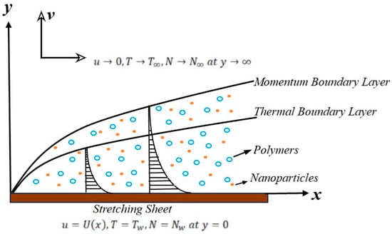
Figure 1.
Geometry of the problem.
In Equations (2)–(5), and are the velocity components, is the density of the fluid, is the thermal diffusivity, is the volumetric volume expansion coefficient of the nanofluid, and and are the thermophoretic diffusion and Brownian diffusion coefficient, respectively. Also, is the shear stress that is correlated to the rate of strain nonlinearly in unique forms for different non-Newtonian fluids.
The appropriate boundary conditions of the problem are as follows [25]:
Larson et al. [26] found out that the friction coefficient of the fluid depends on the shape of the polymer. The value of this coefficient is small when the polymers are in the equilibrium state and large when the polymers are stretched. Hence the relaxation time increases with the stretching of the polymers. is a linear function of the end-to-end distance vector of polymers, .
where is the relaxation time of the polymers in the equilibrium shape and is a positive parameter. In the equilibrium state, and is equal to and when there is stretching, and .
Understanding the behavior of a polymeric chain affected by a fluid flow is the first step in the study of polymer transport. When polymers are placed in a flow, they deform and stretch. Two effects determine the deformation of polymers; their stretching due to the velocity gradients and the elastic relaxation towards the equilibrium shape [4]. In the presence of polymers, even when they are not stretched, the viscosity of the solution increases. Now, the kinematic viscosity of the polymer solution without the stretching can be written as, . To proceed further, we transform our equations into ordinary differential equations using appropriate similarity transformations. For the stretching velocity of the form; , we have [25]:
and the independent variable
Equation (3) has unique forms for different non-Newtonian fluids models. Here, we will be using two models, Reiner–Philippoff and Powell–Eyring, to study the effects of polymers on the flow and heat transfer of the nanofluid and concentration of nanoparticles by using a non-Newtonian fluid as a base fluid.
2.1. Reiner–Philippoff Fluid
The stress deformation of a Reiner–Philippoff fluid is expressed as [25]:
where is the reference shear stress, and is the zero and upper Newtonian limiting viscosity, respectively. The Reiner–Philippoff fluid model is one of the few models that exhibits all the pseudoplastic, Newtonian, and dilatant behaviors.
The transformed Equations (3)–(5) and (8) can be written as:
where is the Weissenberg number, which is the ratio of elastic forces to the viscous forces, and is the Reynolds number, the ratio of inertial forces to the viscous forces. By substituting such that is the plate’s total length, we have:
and is a function of the concentration of the polymers and and are the Reiner–Philippoff model parameters, is the Prandtl number, is the Lewis number, is the Brownian motion parameter, and is the thermophoretic diffusion parameter, which are expressed as [25]:
The boundary conditions transform to:
For , the above problem reduces for the flow of Newtonian fluid and when , we get the flow of a Reiner–Philippoff fluid without polymers.
2.2. Powell–Eyring Fluid
For a Powell–Eyring fluid, we have the following stress-strain relationship [27]:
where is the dynamic viscosity, and and are material constants. Considering the second-order approximation of the above function [27]:
where
The momentum equation for a Powell–Eyring fluid in the presence of polymers becomes,
In the case of the Powell–Eyring model, we apply the same transformations as above, and the transformed Equation (17) attains the form:
where and are the fluid parameters and can be expressed as:
Equations (4) and (5) and the boundary conditions remain the same for the model.
2.3. Polymers End-to-End Distance Vector
To proceed further, we must provide the momentum equation with specific information on . Neglecting the thermal noise, we obtain the following equations for the components of a dimensionless polymer’s end-to-end distance vector [7]:
where is the angle of equilibrium orientation and and . We assume that the polymers follow streamlines of the flow so that:
Now, Equations (19) and (20) take the form:
The quantity is the average of over the polymers in a small region. This ensemble average is the same as an average over , which is uniformly distributed in , thus . It is observed that the equation of motion remains unchanged on reflection and inversion, thus averaging upon is the same as averaging upon . If and are values of and at , Equations (22) and (23) take the form:
And thus we have:
where
with Moreover, we have the viscosity as
and the polymeric solution’s total viscosity is:
Substituting the expression of from Equation (26) in (9) and (18), we have for the Reiner–Philippoff model:
and for the Powell–Eyring model:
Solving (24), (25), and (27)–(29), and then with (30) gives for the polymeric flow for Reiner–Philippoff and Powell–Eyring fluids, respectively.
3. Solution Methodology
In this study, the problem is solved using a numerical method iteratively. To obtain the solution to the problem without the presence of polymers, a nonlinear shooting method with a subroutine of the Runge–Kutta scheme is used, and the results are then utilized to solve Equations (24) and (25) for and . The expression for is obtained from (27), and this is used to solve (28), (29), and then with (30), again using the shooting method. The solution of , the velocity profile for polymeric flow, attained from (28), (29), and (30), is then used in (24) and (25) to obtain a modified . The convergence of the iterative scheme is depicted in Figure 2, which shows that convergence is achieved after just a few iterations. Finally, by using the solution of the momentum equation, the temperature and concentration profiles of the problem are obtained. To clarify the numerical method used to solve the set of equations for the given model, Figure 3 is presented, which shows the step-by-step approach.
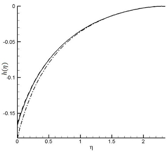
Figure 2.
Result of after the first (dashed-dot), second (dashed), and sixth (solid) iteration with , , , , , , and .
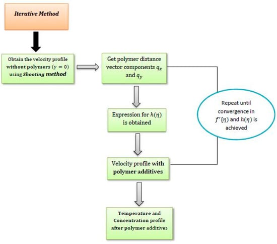
Figure 3.
Interpretation of the numerical solution of the model.
4. Results and Discussions
This section investigates how polymers affect the drag coefficient, Nusselt number, and Sherwood number of non-Newtonian nanofluids. We present graphs for both the Reiner–Philippoff and Powell–Eyring models.
4.1. Impact of Polymers on Drag Coefficient
The skin friction for non-Newtonian fluids is influenced by various factors, including the type of fluid, its rheological properties, and the presence of polymers. Understanding these factors is crucial for predicting and optimizing the flow behavior of non-Newtonian fluids in various industrial applications. Skin friction is the shear stress exerted on the surface by the flowing viscous fluid and it can be mathematically expressed as:
where is shear stress at the surface. For a Reiner–Philippoff fluid, can be written as [26]:
and for a Powell–Eyring fluid [27]:
Using Expressions (31) and (32) in (30), skin friction for a Reiner–Philippoff fluid can be expressed as:
and for a Powell–Eyring fluid, we have:
Figure 4 depicts the behavior of skin friction () of the Reiner–Philippoff-based nanofluid in the presence of polymers. Skin friction is plotted against the non-Newtonian fluid parameter, for different values of the polymer concentration parameter. The value corresponds to the flow without the presence of polymers. In the present scenario, the Reiner–Phippoff model acts as dilatant for , pseudoplastic for and becomes Newtonian for . It is observed that skin friction for a dilatant fluid is higher than for a viscous fluid and a viscous fluid bears more skin friction than a pseudoplastic fluid. Also, one can note that skin friction increases with increasing . This implies that the interaction between the polymer molecules and the sliding surface produces higher resistance, which increases skin drag. Figure 5 investigates the skin friction for a Powell–Eyring fluid in the presence of polymers. Skin friction is plotted against the non-Newtonian fluid parameter, , for different values of the polymer concentration parameter. The same behavior is seen as in the case of a Reiner–Philippoff fluid. As we increase the value of the fluid parameter, the skin friction decreases, and increasing the concentration of the polymers increases the skin friction of the fluid flow.
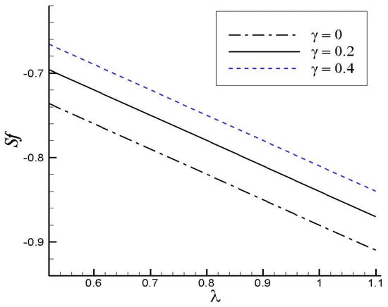
Figure 4.
of a Reiner–Philippoff fluid as a function of the fluid parameter, , for different values of at fixed , , , , , and .
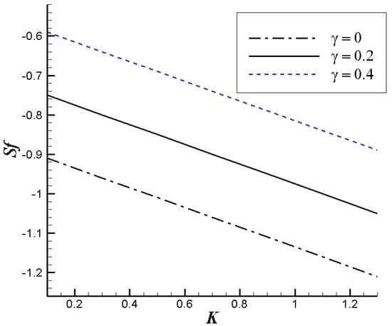
Figure 5.
of a Powell–Eyring fluid as a function of the fluid parameter, for different values of at fixed , , , , , and .
Figure 6 shows the influence of the presence of polymers on the percentage of drag enhancement () of the non-Newtonian-based nanofluid. Drag enhancement is defined as the difference between the skin friction with polymers and without polymers (when ) present. It can be expressed as , being the value without the presence of polymers. In Figure 6, is plotted against the polymer concentration parameter, , for varying non-Newtonian parameter, , and Weissenberg number. The Weissenberg number is a dimensionless number that compares the relaxation time to the characteristic stretching time. It is observed that the greater the concentration of polymers, the greater the resistance between the polymer molecules and the surface, which will increase the rate of enhancement in the skin drag; conversely, this increment decreases with increasing Reiner–Philippoff fluid parameter. Also, increasing implies that the relaxation time increases and the elastic force minimizes, allowing the velocity gradients to stretch the polymers. The fall in with increasing Weissenberg number shows that increasing the relaxation time reduces the enhancement in the drag. The same effects on drag enhancement of varying and are observed for a Powell–Eyring fluid.
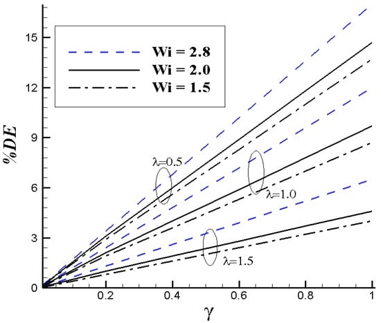
Figure 6.
Effects on the percentage of drag enhancement () due to the presence of polymers as a function of for fixed , , , , , , and for a Reiner–Philippoff fluid.
4.2. Impact of Polymers on Nusselt Number
Another important quantity of interest is the Nusselt number () expressed as [26]:
where is the heat flux defined as:
Using Equation (36) in (35), we get:
which is known as the reduced Nusselt number.
In Figure 7, the behavior of the Nusselt number () of a Reiner–Philippoff-based nanofluid in the presence of polymers is discussed. is plotted against the thermophoresis parameter, for nanoparticles with different values of the polymer concentration parameter. The zero value of corresponds to the flow without the presence of polymers. It is observed that increasing the value of reduces the . This implies that as the thermophoresis parameter increases, it will slow down the process of heat transfer. Also, the addition of polymers in the flow reduces the Nusselt number or the heat flux at the surface. Figure 8 shows plotted against the Brownian diffusion parameter, , for a Powell–Erying fluid. As can be seen, as the rate of diffusion between the particles increases, the heat flux or heat transfer rate decreases. Furthermore, it can be seen that this rate is also affected by increasing polymer concentration in the solution. The diffusion of the polymers in the solution also contributes to decreasing the process of heat transfer.
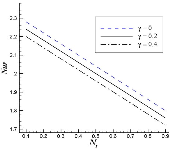
Figure 7.
as a function of for different with , , , , , , and of a Reiner–Philippoff fluid.
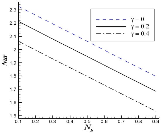
Figure 8.
as a function of for different with , , , , , , and of a Powell–Eyring fluid.
Figure 9 represents the effects of the presence of polymers on the percentage of heat reduction () of the non-Newtonian-based nanofluid flow. Heat reduction is defined as ( being the value without the presence of polymers). In Figure 9, is plotted against the polymer concentration parameter for different values of Weissenberg number and non-Newtonian fluid parameter. This plot shows that if we increase the concentration of polymers in the solution, there is more heat reduction. Similarly, the reduction in with increasing Weissenberg number shows that polymer stretching impedes the heat reduction process of the flow at the surface. The same results for heat reduction with varying and are observed for a Powell–Eyring fluid. Also, the heat reduction rate increases with the increasing value of the Reiner–Philippoff fluid parameter. Figure 10 indicates the influence of the presence of polymers on as a function of for different for a Reiner–Philippoff fluid. It has already been observed that increasing the concentration of polymers in the solution increases heat reduction. One interesting thing to note is that the presence of polymers also affects the concentration of the nanoparticles in the flow. We see that as we increase the value of the Brownian diffusion parameter, , heat reduction at the surface decreases. This implies that as the random movement of the particles increases due to collisions of the different molecules, the heat reduction process is impeded. Figure 11 shows the influence of polymers on for different for a Powell–Eyring fluid. We find that when the value of the thermophoresis parameter increases, the heat transfer reduction at the surface decreases.
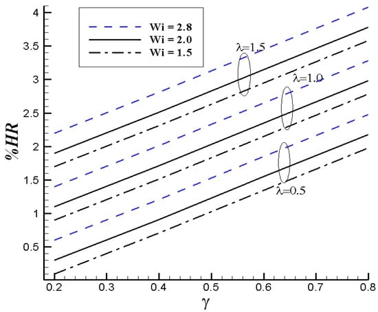
Figure 9.
Effects on the percentage of heat reduction () due to polymers as a function of for fixed , , , , , , and for a Reiner–Philippoff fluid.
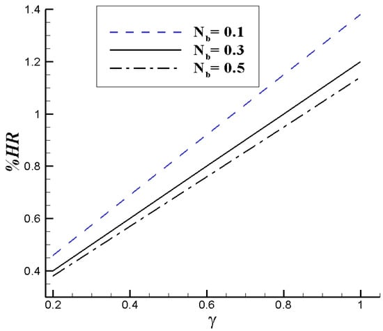
Figure 10.
Effects on the percentage of heat reduction () due to the presence of polymers as a function of for different with , , , , , and for a Reiner–Philippoff fluid.
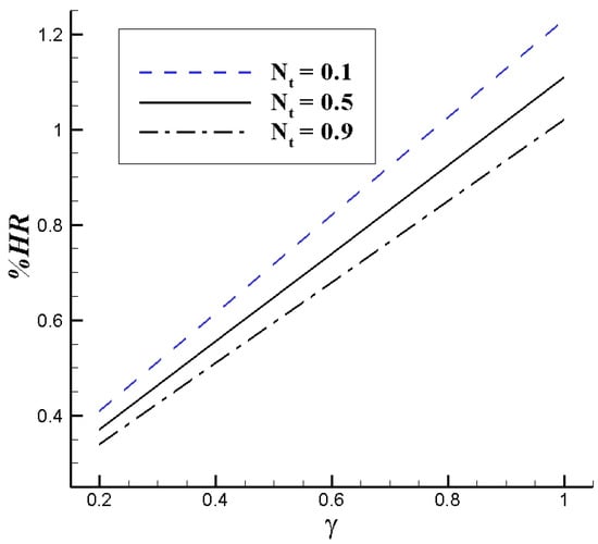
Figure 11.
Effects on the percentage of heat reduction () due to the presence of polymers as a function of for different with , , , , , and for a Powell–Eyring fluid.
4.3. Impact of Polymers on Sherwood Number
Similarly, the Sherwood number can be defined as:
where is the reduced Sherwood number. In Figure 12, the behavior of the Sherwood number () of a Reiner–Philippoff-based nanofluid in the presence of polymers is shown. is plotted against the Brownian diffusion parameter, , due to nanoparticles for different values of the polymer concentration parameter. A zero value of corresponds to the flow without the presence of polymers. It can be seen that increasing the value of increases the . This implies that as the Brownian diffusion parameter increases, convective mass transfer becomes dominant and the Sherwood number increases. Also, the addition of polymers in the flow reduces the Sherwood number or the mass flux at the surface. The same results are seen with the Powell–Eyring model.
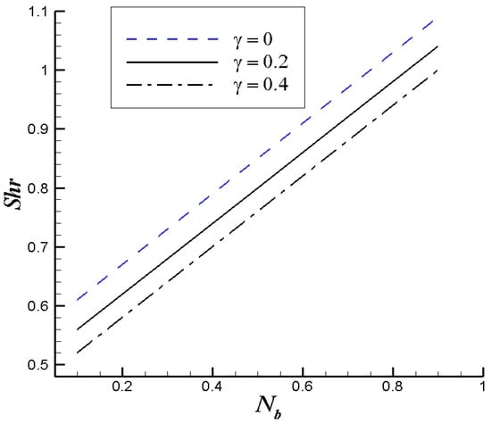
Figure 12.
as a function of for different with , , , , , , and for a Reiner–Philippoff fluid.
Figure 13 presents the effect of the presence of polymers on the percentage of mass transfer reduction () of the flow, which is defined as ( being the value without the presence of polymers). In Figure 13, is plotted against the polymer concentration parameter for different and which shows that if we increase the concentration of polymers in the solution, mass transfer at the surface decreases. Similarly, a decrease in with increasing Weissenberg number shows that polymer stretching also impedes the mass reduction process of the flow at the surface. An increasing non-Newtonian flow parameter also causes a decrease in mass flux in the presence of polymers. In Figure 14, one interesting thing to note is that the polymers also affect the concentration of nanoparticles in the flow. We see that as we increase the value of the Brownian diffusion parameter, , the percentage of mass reduction at the surface increases. This implies that as the random movement of the particles increases due to collisions of the different molecules, mass transfer due to convection becomes dominant and so the reduction process speeds up. Figure 15 shows the influence of the presence of polymers on for different for a Powell–Eyring fluid. We find that when the value of the thermophoresis parameter increases, the heat transfer reduction at the surface decreases.
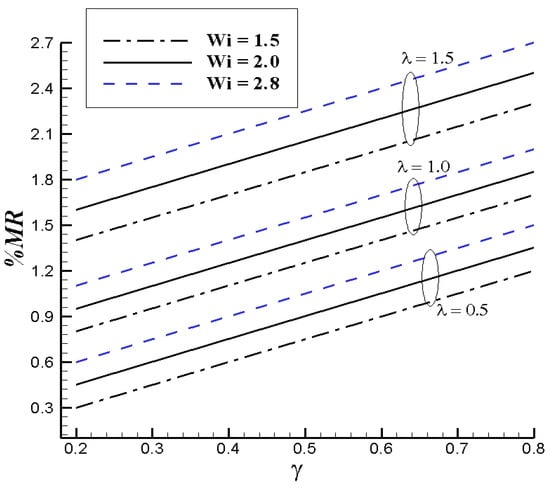
Figure 13.
Effect on of the presence of polymers as a function of for fixed , , , , and for a Reiner–Philippoff fluid.
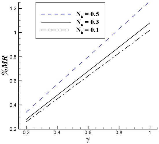
Figure 14.
Effect on % of the presence of polymers as a function of for different with , , , , , and for a Reiner–Philippoff fluid.
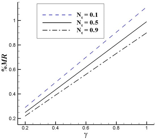
Figure 15.
Effect on of the presence of polymers as a function of for different with , , , , , and for a Powell–Eyring fluid.
All the results presented in this article are in agreement with [7], in which Benzi et al. discussed the heat transport with polymers, and with [26], in which the authors studied the boundary layer flow of a non-Newtonian-based nanofluid.
5. Conclusions
In summary, this theoretical study investigated the influence of the presence of polymers on the boundary layer flow of non-Newtonian-based nanofluids. Various non-Newtonian fluid models and a molecular approach were employed to derive the governing equations. These equations were then solved numerically, and the results were analyzed. The key findings are as follows:
- The addition of polymers to a non-Newtonian fluid generally increases the viscosity of the solution, although the viscosity reduction occurs to a lesser extent with polymer stretching.
- The introduction of polymers in non-Newtonian-based nanofluids leads to an increase in the drag coefficient and a decrease in the Nusselt number and Sherwood number.
- The concentration of polymers in the solution has a direct impact on skin friction, showing that an increase in polymer concentration results in higher skin friction.
- Higher polymer concentrations correspond to greater drag enhancement, as well as increased heat and mass reduction.
- The effects of thermophoresis and Brownian diffusion are not limited to reduced Nusselt number and Sherwood number; they also influence the behavior of the polymers.
This study primarily focused on the measurement of skin drag, heat transfer, and mass transfer in non-Newtonian-based nanofluids with polymer additives. Subjects that were not explored in this study present several avenues for further research, including investigating viscous dissipation effects and entropy generation and conducting experimental studies to support or challenge our findings.
Author Contributions
Software and writing—original draft preparation, A.S.; Conceptualization, and methodology, A.A.; validation and formal analysis, R.K.; writing—review and editing, R.N. All authors have read and agreed to the published version of the manuscript.
Funding
This research received no external funding.
Data Availability Statement
No new data were created or analyzed in this study. Data sharing is not applicable to this article.
Conflicts of Interest
The authors declare no conflict of interest.
Nomenclature
| viscosity due to polymers | |
| relaxation time | |
| dynamic viscosity | |
| Weissenberg number. | |
| polymer concentration parameter | |
| Thermophoretic diffusion coefficient | |
| Prandtl number | |
| stretching velocity | |
| dimensionless stream function | |
| relaxation time in equilibrium | |
| zero and upper Newtonian limiting viscosity | |
| ambient temperature and concentration | |
| reduced Nusselt number | |
| material fluid constants | |
| density ( | |
| thermal diffusivity . | |
| Reiner–Philippoff fluid parameter | |
| Reynolds number | |
| Brownian diffusion coefficient ( | |
| thermophoresis diffusion coefficient | |
| Brownian diffusion coefficient. | |
| dimensional fluid temperature | |
| Powell–Eyring fluid parameter | |
| Lewis number | |
| temperature and concentration at the surface | |
| skin friction coefficient | |
| dimensional velocity components | |
| material fluid constants |
References
- Apmann, K.; Fulmer, R.; Soto, A.; Vafaei, S. Thermal Conductivity and Viscosity: Review and Optimization of Effects of Nanoparticles. Materials 2021, 14, 1291. [Google Scholar] [CrossRef] [PubMed]
- Mackay, M.E.; Dao, T.T.; Tuteja, A.; Ho, D.L.; van Horn, B.; Kim, H.C.; Hawker, C.J. Nanoscale effects leading to non-Einstein-like decrease in viscosity. Nat. Mater. 2003, 2, 762–766. [Google Scholar] [CrossRef] [PubMed]
- Bird, R.B.; Giacomin, A.J. Polymer fluid dynamics: Continuum and molecular approaches. Annu. Rev. Chem. Biomol. Eng. 2016, 7, 479–507. [Google Scholar] [CrossRef] [PubMed]
- Celani, A.; Musacchio, S.; Vincenzi, D. Polymer transport in random flow. J.Stat. Phys. 2005, 118, 531–554. [Google Scholar]
- Al-Yaari, M.; Soleimani, A.; Abu-Sharkh, B.; Al-Mubaiyedh, U.; Al-Sarkhi, A. Effect of drag reducing polymers on oil–water flow in a horizontal pipe. Int. J. Multiph. Flow. 2009, 35, 516–524. [Google Scholar] [CrossRef]
- Ahlers, G.; Nikolaenko, A. Effect of a polymer additive on heat transport in turbulent Rayleigh-Bénard convection. Phys. Rev. Lett. 2010, 104, 034503. [Google Scholar]
- Benzi, R.; Ching, E.S.; Chu, V.W. Heat transport by laminar boundary layer flow with polymers. J. Fluid Mech. 2012, 696, 330–344. [Google Scholar] [CrossRef]
- Athar, M.; Ahmad, A. Behavior of fluid flow and heat transfer induced by a stretching surface in the presence of polymers. Phys. Scr. 2021, 96, 13. [Google Scholar] [CrossRef]
- Marenduzzo, D.; Micheletti, C.; Seyed-Allaei, H.; Trovato, A.; Maritan, A. Continuum model for polymers with finite thickness. J. Phys. A Math. Gen. 2005, 38, L277. [Google Scholar] [CrossRef]
- Doufas, A.K.; Dairanieh, I.S.; McHugh, A.J. A continuum model for flow-induced crystallization of polymer melts. J. Rheol. 1999, 43, 85–109. [Google Scholar] [CrossRef]
- Zhang, Y.; Zhang, Z.; Yang, J.; Yue, Y.; Zhang, H. A Review of Recent Advances in Superhydrophobic Surfaces and Their Applications in Drag Reduction and Heat Transfer. Nanomaterials 2022, 12, 44. [Google Scholar]
- Ahmad, A.; Ishaq, A.; Khan, Y. Influence of FENE-P fluid on drag reduction and heat transfer past a magnetized surface. Int. J. Mod. Phys. B 2022, 36, 2250145. [Google Scholar] [CrossRef]
- Tiwari, R.K.; Das, M.K. Heat transfer augmentation in a two-sided lid-driven differentially heated square cavity utilizing nanofluids. Int. J. Heat Mass Transf. 2007, 50, 2002–2018. [Google Scholar]
- Buongiorno, J. Convective transport in nanofluids. J. Heat Transf. 2006, 128, 240–250. [Google Scholar] [CrossRef]
- Eastman, J.A.; Choi SU, S.; Li, S.; Yu, W.; Thompson, L.J. Anomalously increased effective thermal conductivities of ethylene glycol-based nanofluids containing copper nanoparticles. Appl. Phys. Lett. 2001, 78, 718–720. [Google Scholar] [CrossRef]
- Sheikholeslami, M.; Rashidi, M.M.; Hayat, T.; Ganji, D.D. Free convection of magnetic nanofluid considering MFD viscosity effect. J. Mol. Liq. 2016, 219, 79–85. [Google Scholar] [CrossRef]
- Abbas, W.; Sayed, E.A. Hall current and joule heating effects on free convection flow of a nanofluid over a vertical cone in presence of thermal radiation. Therm. Sci. 2017, 21, 863–876. [Google Scholar] [CrossRef]
- Mahanthesh, B.; Gireesha, B.J.; Animasaun, I.L.; Muhammad, T.; Shashikumar, N.S. MHD flow of SWCNT and MWCNT nanoliquids past a rotating stretchable disk with thermal and exponential space dependent heat source. Phys. Scr. 2019, 94, 085214. [Google Scholar] [CrossRef]
- Shehzad, N.; Zeeshan, A.; Ellahi, R.; Vafai, K. Convective heat transfer of nanofluid in a wavy channel: Buongiorno’s mathematical model. J. Mol. Liq. 2016, 219, 970–977. [Google Scholar] [CrossRef]
- Zheng, L.; Zhang, C.; Zhang, X.; Zhang, J. Flow and radiation heat transfer of a nanofluid over a stretching sheet with velocity slip and temperature jump in porous medium. J. Frankl. Inst. 2013, 350, 2142–2156. [Google Scholar] [CrossRef]
- Jahan, S.; Sakidin, H.; Nazar, R.; Pop, I. Analysis of heat transfer in nanofluid past a convectively heated permeable stretching/shrinking sheet with regression and stability analyses. Results Phys. 2018, 10, 195–202. [Google Scholar] [CrossRef]
- Raju CS, K.; Ahammad, N.A.; Sajjan, K.; Shah, N.A.; Yook, S.J.; Kumar, M.D. Nonlinear movements of axisymmetric ternary hybrid nanofluids in a thermally radiated expanding or contracting permeable Darcy Walls with different shapes and densities: Simple linear regression. Int. Commun. Heat Mass Transf. 2022, 135, 106110. [Google Scholar]
- Kumar, M.D.; Raju CS, K.; Sajjan, K.; El-Zahar, E.R.; Shah, N.A. Linear and quadratic convection on 3D flow with transpiration and hybrid nanoparticles. Int. Commun. Heat Mass Transf. 2022, 134, 105995. [Google Scholar]
- Ahmad, A.; Athar, M.; Khan, Y. Influence of polymers on drag and heat transfer of nanofluid past stretching surface: A molecular approach. J. Cent. South Univ. 2022, 29, 3912–3924. [Google Scholar] [CrossRef]
- Ahmad, A. Flow of ReinerPhilippoff based nano-fluid past a stretching sheet. J. Mol. Liq. 2016, 219, 643–646. [Google Scholar]
- Larson, R.G.; Perkins, T.T.; Smith, D.E.; Chu, S. Hydrodynamics of a DNA molecule in a flow field. Phys. Rev. 1997, 55, 1794. [Google Scholar]
- Jalil, M.; Asghar, S.; Imran, S.M. Self similar solutions for the flow and heat transfer of Powell-Eyring fluid over a moving surface in a parallel free stream. Int. J. Heat Mass Transf. 2013, 65, 73–79. [Google Scholar]


Disclaimer/Publisher’s Note: The statements, opinions and data contained in all publications are solely those of the individual author(s) and contributor(s) and not of MDPI and/or the editor(s). MDPI and/or the editor(s) disclaim responsibility for any injury to people or property resulting from any ideas, methods, instructions or products referred to in the content. |
© 2023 by the authors. Licensee MDPI, Basel, Switzerland. This article is an open access article distributed under the terms and conditions of the Creative Commons Attribution (CC BY) license (https://creativecommons.org/licenses/by/4.0/).