Study on a Novel Strategy for High-Quality Grinding Surface Based on the Coefficient of Friction

Abstract

Surface quality has a significant impact on the service life of machine parts. Grinding is often the last process to ensure surface quality and accuracy of material formation. In this study, a high-quality surface was developed by determining the coefficient of friction in grinding a quartz fiber-reinforced silica ceramic composite. By processing the physical signals in the grinding process, a multi-objective function was established by considering grinding parameters, i.e., surface roughness, coefficient of friction, active energy consumption, and effective grinding time. The weight vector coefficients of the sub-objective functions were optimized through a multi-objective evolutionary algorithm based on the decomposition (MOEA/D) algorithm. The genetic algorithm was used to optimize the process parameters of the multi-objective function, and the optimal range for the coefficient of friction was determined to be 0.197~0.216. The experimental results indicated that when the coefficient of friction tends to 0.197, the distribution distance of the microscopic data points on the surface profile is small and the distribution uniformity is good. When the coefficient of friction tends to 0.216, the surface profile shows a good periodic characteristic. The quality of a grinding surface depends on the uniformity and periodicity of the surface’s topography. The coefficient of friction explained the typical physical characteristics of high-quality grinding surfaces. The multi-objective optimization function was even more important for the subsequent high-quality machining of mechanical parts to provide guidance and reference significance.

1. Introduction

Quartz fiber-reinforced silica ceramic composite has been successfully used in building materials, the chemical industry, national defense, and other sectors [1,2] due to its low thermal conductivity, small expansion coefficient, and high-temperature resistance. However, low mechanical strength and high brittleness make it a difficult-to-cut material with poor surface quality [3]. In surface processing of this material, grinding is one of the most widely employed machining processes due to its high precision and stable surface quality. The range of force ratios taken during grinding is crucial due to the brittleness of the ceramic composite. In comparison with other machining processes, grinding consumes high amounts of energy with a low efficiency for the same level of material volume removal [4]. Some strategies have been used to improve the quality of grinding surfaces, such as surface modification or the application of coating techniques on the substrate surface [5]. However, both surface modification and surface application coating technologies pose some environmental problems to a greater or lesser extent [6]. Under the strategic target of “carbon neutrality”, energy saving and carbon emission reduction have become part of a global consensus in the surface machining process. Therefore, it is particularly important to investigate the physical mechanisms of molding for high surface quality.

With the advancement of science and technology, intelligent monitoring technology has developed rapidly [7,8]. By analyzing and processing the signals collected by various sensors, the grinding process can be better monitored. Wang et al. [9] innovatively proposed a signal processing method based on fuzzy C-average clustering. This method can accurately predict the subsurface damage depth and surface quality in ultra-precision grinding of single-crystal silicon. Wang et al. [10] utilized multiple transformation forms of raw AE signals to monitor materials’ surface behavior and developed a force model to explain forces under different removal modes. Ling et al. [11] used different types of new sandpaper to grind the surface of an alloy and investigated the effect of the grinding treatment on the surface properties and deformation microstructure. Zhang et al. [12] introduced a novel data-driven model using an optimized pruned extreme learning machine. Real-time quantitative monitoring of abrasive belt conditions can be achieved in robotic grinding systems by a novel method based on acoustic signals. Tian et al. [13] developed a portable power monitoring system for grinding signal acquisition, feature extraction, and data calculation to improve the surface quality achieved by grinding.

To characterize the actual wear state of micro-grinding wheels, a novel monitoring method was proposed based on the variable cutting stiffness with a fusion analysis of forces and system vibration signals [14,15]. Warren et al. [16] applied a discrete wavelet decomposition procedure to extract discriminative features from original acoustic emission (AE) signals. And the state of the grinding wheels was monitored through the wavelet-based AE signal. Based on the physical characteristics of grinding, some achievements have been made in ensuring surface quality, saving energy, and improving efficiency. Ma et al. [17] first proposed the concept of “relative extreme value error” to judge the influence sensitivity of technical factors on surface roughness. Based on the analysis of cracks and grinding kinetics, Yao et al. [18] established a relationship between surface roughness and subsurface crack depth. Kong et al. [19] introduced an effective feature extraction method through the combination of PCA and KPCA_IRBF, which can be utilized for surface roughness prediction. Meng et al. [20] presented an innovative dynamic force model for precision grinding with micro-structured grinding wheels. Li et al. [21] modeled grinding temperature with a genetic association analysis tool (PGA) and regarded it as the main constraint for the inverse problem while modeling the grinding surface roughness and grinding continuity as auxiliary constraints. The ability of high-accuracy Artificial Neural Networks (ANNs) regarding feature classification, especially on nonlinear patterns, was considered [22]. Dai et al. [23] studied the effect of grinding speed on grinding temperature and power consumption and analyzed the grinding surface performance from the perspective of undeformed chip thickness. Wang et al. [24] developed a nonparametric model based on an improved adaptive Artificial Neural Network (aANN) to predict surface quality, machining time, total power consumption, and effective power consumption.

The methodological strategies adopted in the above studies have optimized the grinding surface quality to varying degrees, but few investigations have been conducted to evaluate the superiority and inferiority of the microscopic data on the machined surface. This study intends to explore the typical physical characteristics of high-quality surfaces through the coefficient of friction, under the premise of non-pollution to the environment and controllable operation. A multi-objective numerical function for comprehensive evaluation of the grinding surface was established. The value of the coefficient of friction directly affects workpiece surface quality, which is conducive to the improvement of the service performance of processed parts. Within a suitable range of the coefficient of friction, a uniformly distributed and periodic machined surface profile with a R_a of about 0.3 μm can be obtained. This research has great significance for solving problems of high surface quality and low energy consumption in grinding.

2. Materials and Methods

2.1. Experimental Equipment

A grinding experimental platform was established for multi-feature signal acquisition; see Figure 1a. It mainly consisted of a CNC surface grinder (SMART-B818III, Falcon Machine Tools Co., Ltd., Changhua County, Taiwan), a portable power cell (PPC-3, Load Controls Inc., Sturbridge, MA, USA), and a multicomponent dynamometer (Type 9527B, Kistler Holding AG, Winterthur, Switzerland). The PPC-3 has three Hall-effect current sensors and three voltage sensors. The outputs of the PPC-3 are 0–20 mA in current and 0–10 V in voltage. The in-process current and voltage signals were measured by the PPC-3, and effective powers were calculated from the measured data. The dynamometer, the measurement error of which is one percent, can simultaneously measure force and torque in the X, Y, and Z axes of the grinder. Power signals and force signals were collected online at 1000 Hz and 2000 Hz, respectively. The surface roughness Ra and surface profile curve were measured by a roughness tester (TIME3200, TIME Group Inc., Beijing, China). After each grinding test, six positions on the machined surface were selected to measure the roughness R_a; see Figure 1b. Ignoring the maximum and minimum values, the other four measured data points were averaged for each set of experiments. The workpiece material was a quartz fiber-reinforced silica ceramic composite with dimensions of 50 × 50 × 25 mm. A resin-bonded diamond flat grinding wheel was used with an outer diameter of 200 mm and a thickness of 10 mm. The basic size of abrasive grains was about 20 μm [25].

2.2. Experimental Scheme

The grinding surface quality, energy consumption, force, and cost are influenced by the linear speed of the grinding wheel v_s (m/min), workpiece infeed speed v_w (mm/min), and grinding depth a_p (μm). In this work, a full factorial experiment with these three factors and five levels was designed, and three-fifths of the total tests were randomly selected. The linear speed of the grinding wheel was varied from 1000 m/min to 1800 m/min, the workpiece infeed speed was varied from 1000 mm/min to 5000 mm/min, and the grinding depth was varied from 4 µm to 12 µm, as listed in

Table 1. Experimental parameters of grinding tests.

Parameters	Values
The linear speed of the grinding wheel vs (m/min)	1000(S1), 1200(S2), 1400(S3), 1600(S4), 1800(S5)
Workpiece speed vw (mm/min)	1000(F1), 2000(F2), 3000(F3), 4000(F4), 5000(F5)
Grinding depth ap (μm)	4(D1), 6(D2), 8(D3), 10(D4), 12(D5)

.

2.3. Signal Processing

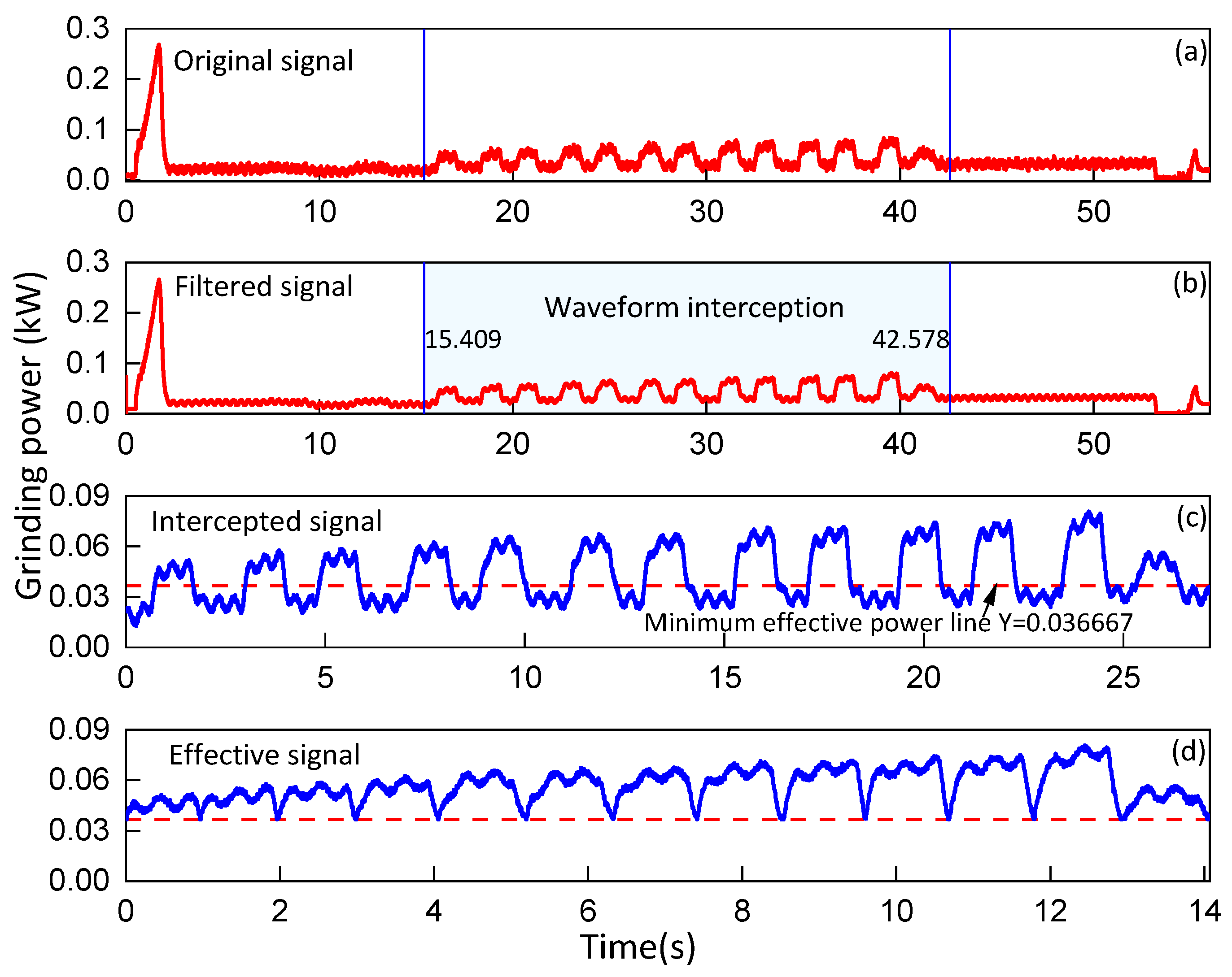
2.3.1. Grinding Force Signal Processing

The surface quality and energy consumption can be affected by grinding forces directly. It is critical to analyze and process three-component force signals. The normal force is closely related to the compressive strength of the grinding wheel and system rigidity. The tangential force has a direct impact on effective power in grinding. The axial force is the force along the axis of the grinding wheel. Insufficient contact signal removal, drift signal correction, signal denoising strategy, and effective normal force signal acquisition have been elaborated on in previous work [26]. Figure 2 shows the processing method of grinding force signals. It is observed in Figure 2a that the signals of tangential force and normal force are oppositely distributed along the time axis. The negative value of tangential force indicates the direction of the force. A discrete-time Fourier transform (DTFT) was employed to monitor the frequency domain curves of the force as follows:

$$X({\mathrm{e}}^{\mathrm{j}\omega })={\displaystyle {\sum }_{n=0}^{n-1}x[n]}\cdot {\mathrm{e}}^{-\mathrm{j}\omega n}$$

(1)

where X(e^jω) is the frequency domain function of the grinding force signal, x[n] is the time series of the grinding force signal, n is the index of the position of the grinding force data point, j is the imaginary unit, and ω is the grinding force signal frequency variable. The frequency distribution was analyzed to establish a low cut-off frequency value. The Chebyshev filter transfer function is as follows:

$${\left|G_M(j\omega )\right|}^2=\frac{1}{1+{\epsilon }^2{T}_M^2(\omega /{\omega }_0)}$$

(2)

where ω₀ is the grinding force signal’s expected cut-off frequency, ε is the grinding force signal wave coefficient which is a positive number less than 1, and T_M is a Chebyshev polynomial of order M.

The original force signals were filtered at an expected cut-off frequency, as shown in Figure 2b. Afterwards, a local amplification component function was used to find the minimum normal force and maximum tangential force. The signals far away from the mini/max value were extracted by the for loop. For tangential force, the absolute value of the extracted signal was taken. By removing invalid interval signals, an effective force signal was formed; see Figure 2c,d. The effective grinding time for each test can be obtained from the effective force signals. The mean coefficient of friction was calculated from the average ratio of the effective tangential force to the effective normal force.

2.3.2. Grinding Power Signal Processing

Grinding wheel abrasives with a large negative angle make the grinding process consume more energy than other machining processes under the same material removal rate [27,28]. Visualization of energy consumption by monitoring power signals online is beneficial to the energy conservation of machine tools. The active power is the actual and irreversible power of the machine tool. It reflects the amount of electric energy converted into other energy in unit time. The extraction strategy of the active power signal is crucial for the analysis of power signals detected during grinding.

In order to fully collect the power signal during grinding, PPC-3 was used to measure the power signal online in advance; see Figure 3a. The power signal was filtered through Equations (1) and (2) in the air grinding stage to achieve a denoising operation; see Figure 3b. The power signal segments during grinding were obtained by longitudinal line selection. The non-grinding power signal under the longitudinal line was removed. The minimum effective power during grinding was determined by a horizontal line; see Figure 3c. All arrays in the power signal larger than the value were extracted by the program to form an effective power array; see Figure 3d. Based on the effective power and time arrays, the grinding active energy consumption can be obtained by numerical integration:

$$E_{\mathrm{active}}={\displaystyle {\int }_0^{T}P(t)dt}$$

(3)

where E_active is the active power, P(t) is the power signal, and t is the time.

3. Results

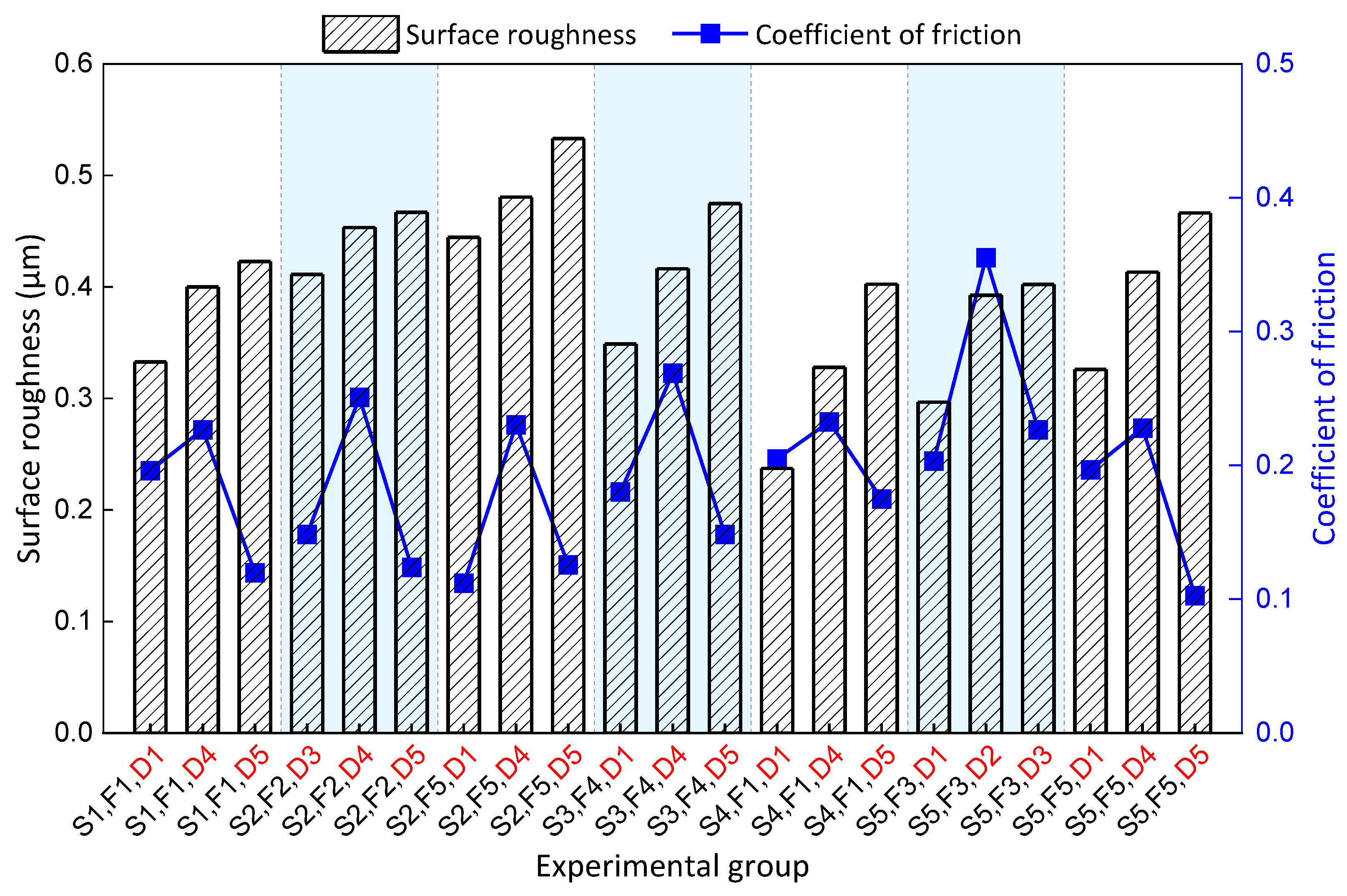
3.1. Experimental Results

A full-factor experiment of v_s, v_w, and a_p was designed in five levels. A total of 125 sets of experimental parameters were obtained. Three-fifths of experimental groups, i.e., 75 groups, were selected stochastically to generate irregular samples. The processed force signal and power signal were analyzed and the experimental results are listed in

Table 2. Grinding parameters and output results.

No.	Inputs			Outputs
	vs (m/min)	vw (mm/min)	ap (μm)	Ra (μm)	u	Ea (J)	T (s)
1	1000	1000	4	0.333	0.196	520.824	29.945
2	1000	1000	10	0.400	0.227	538.088	29.690
3	1000	1000	12	0.423	0.120	626.641	29.963
4	1000	2000	4	0.426	0.159	119.739	14.982
5	1000	2000	6	0.419	0.236	147.500	14.956
6	1000	2000	8	0.424	0.181	168.877	15.019
7	1000	3000	6	0.433	0.106	72.429	10.004
8	1000	3000	8	0.465	0.132	83.263	9.987
9	1000	3000	12	0.513	0.116	116.740	9.934
10	1000	4000	4	0.427	0.130	58.609	7.510
11	1000	4000	10	0.436	0.164	95.176	7.389
12	1000	4000	12	0.529	0.156	115.372	7.481
13	1000	5000	6	0.462	0.069	72.429	5.975
14	1000	5000	8	0.466	0.177	76.690	6.342
15	1000	5000	12	0.539	0.144	96.517	5.958
16	1200	1000	4	0.305	0.140	486.283	30.353
17	1200	1000	6	0.390	0.140	511.823	30.042
18	1200	1000	8	0.401	0.134	567.206	29.926
19	1200	2000	8	0.411	0.148	167.374	11.738
20	1200	2000	10	0.453	0.251	216.624	15.019
21	1200	2000	12	0.467	0.124	317.837	15.034
22	1200	3000	4	0.440	0.053	63.669	9.980
23	1200	3000	10	0.464	0.112	71.240	9.780
24	1200	3000	12	0.479	0.111	202.890	9.967
25	1200	4000	6	0.469	0.126	69.445	7.453
26	1200	4000	8	0.501	0.127	102.964	7.454
27	1200	4000	12	0.491	0.126	108.551	7.365
28	1200	5000	4	0.445	0.112	44.026	5.310
29	1200	5000	10	0.481	0.230	46.059	5.754
30	1200	5000	12	0.533	0.126	69.332	5.961
31	1400	1000	6	0.376	0.107	518.141	29.710
32	1400	1000	8	0.400	0.167	544.445	28.751
33	1400	1000	12	0.415	0.135	568.541	28.738
34	1400	2000	4	0.313	0.071	136.096	12.854
35	1400	2000	10	0.397	0.303	146.993	13.189
36	1400	2000	12	0.437	0.260	159.001	14.559
37	1400	3000	6	0.394	0.060	162.067	9.769
38	1400	3000	8	0.432	0.149	189.511	9.805
39	1400	3000	12	0.440	0.131	144.624	9.943
40	1400	4000	4	0.349	0.180	73.428	7.117
41	1400	4000	10	0.416	0.269	91.638	7.341
42	1400	4000	12	0.475	0.149	130.246	7.446
43	1400	5000	4	0.418	0.096	43.957	6.001
44	1400	5000	6	0.430	0.218	67.381	5.984
45	1400	5000	8	0.452	0.155	84.441	5.334
46	1600	1000	4	0.237	0.205	468.124	29.853
47	1600	1000	10	0.328	0.233	548.139	30.351
48	1600	1000	12	0.403	0.175	564.990	30.643
49	1600	2000	6	0.366	0.098	138.741	15.092
50	1600	2000	8	0.388	0.343	151.043	15.099
51	1600	2000	12	0.419	0.135	178.248	15.042
52	1600	3000	4	0.311	0.064	97.888	9.906
53	1600	3000	10	0.400	0.108	111.350	9.979
54	1600	3000	12	0.440	0.081	125.653	9.958
55	1600	4000	4	0.341	0.102	27.717	7.381
56	1600	4000	6	0.434	0.112	37.726	7.533
57	1600	4000	8	0.432	0.143	89.867	7.475
58	1600	5000	8	0.450	0.141	47.901	6.010
59	1600	5000	10	0.480	0.146	63.151	5.969
60	1600	5000	12	0.471	0.141	76.120	5.944
61	1800	1000	6	0.371	0.142	492.783	30.104
62	1800	1000	8	0.393	0.154	510.063	29.023
63	1800	1000	12	0.344	0.059	688.878	30.22
64	1800	2000	4	0.287	0.139	116.907	14.702
65	1800	2000	10	0.373	0.469	144.436	14.891
66	1800	2000	12	0.416	0.174	165.680	14.857
67	1800	3000	4	0.297	0.203	71.907	9.950
68	1800	3000	6	0.393	0.355	74.378	10.046
69	1800	3000	8	0.402	0.227	75.018	10.102
70	1800	4000	6	0.426	0.106	66.879	7.464
71	1800	4000	8	0.404	0.147	69.806	7.546
72	1800	4000	12	0.419	0.137	112.556	7.619
73	1800	5000	4	0.326	0.197	45.776	5.534
74	1800	5000	10	0.413	0.228	62.568	6.008
75	1800	5000	12	0.466	0.103	78.477	5.927

. It includes surface roughness R_a (μm), coefficient of friction u (Ft/Fn), active energy consumption E_a (J), and effective grinding time T (s).

3.2. Interaction among Evaluation Indicators

The evaluation indicators include surface roughness, coefficient of friction, active energy consumption, and effective grinding time, as listed in Table 2. Exploring the relationship between evaluation indicators is beneficial to promoting the grinding process toward a goal of high surface quality with high efficiency and low energy consumption. The coefficient of friction is a comprehensive reflection of tangential force and normal force, which may affect the surface quality. Another parameter that has a big influence on surface quality is the grinding depth. It is significant to investigate the relationship between the coefficient of friction and surface roughness under changes in the grinding depth for the same linear speed of the grinding wheel and the same workpiece infeed speed. A total of 21 sets of experimental data from seven groups were selected and plotted; see Figure 4. It shows that with an increasing grinding depth, the coefficient of friction increased and then decreased, and the surface roughness increased. It is clear that a high coefficient of friction leads to bad surface roughness. The smallest surface roughness is not related to the smallest coefficient of friction for each group. Therefore, it is crucial to analyze the correlation between the coefficient of friction and surface roughness.

Compared with the linear speed of the grinding wheel and grinding depth, the workpiece infeed speed has a greater impact on the active energy consumption and effective grinding time [29]. The relationship between active energy consumption and effective grinding time was analyzed. A total of 21 experimental sets in seven control groups were selected and plotted in Figure 5 and Figure 6. It was found that the smaller the infeed speed of the workpiece, the more active energy and grinding time were consumed. Better surface roughness was always associated with a larger active energy consumption or a longer effective grinding time.

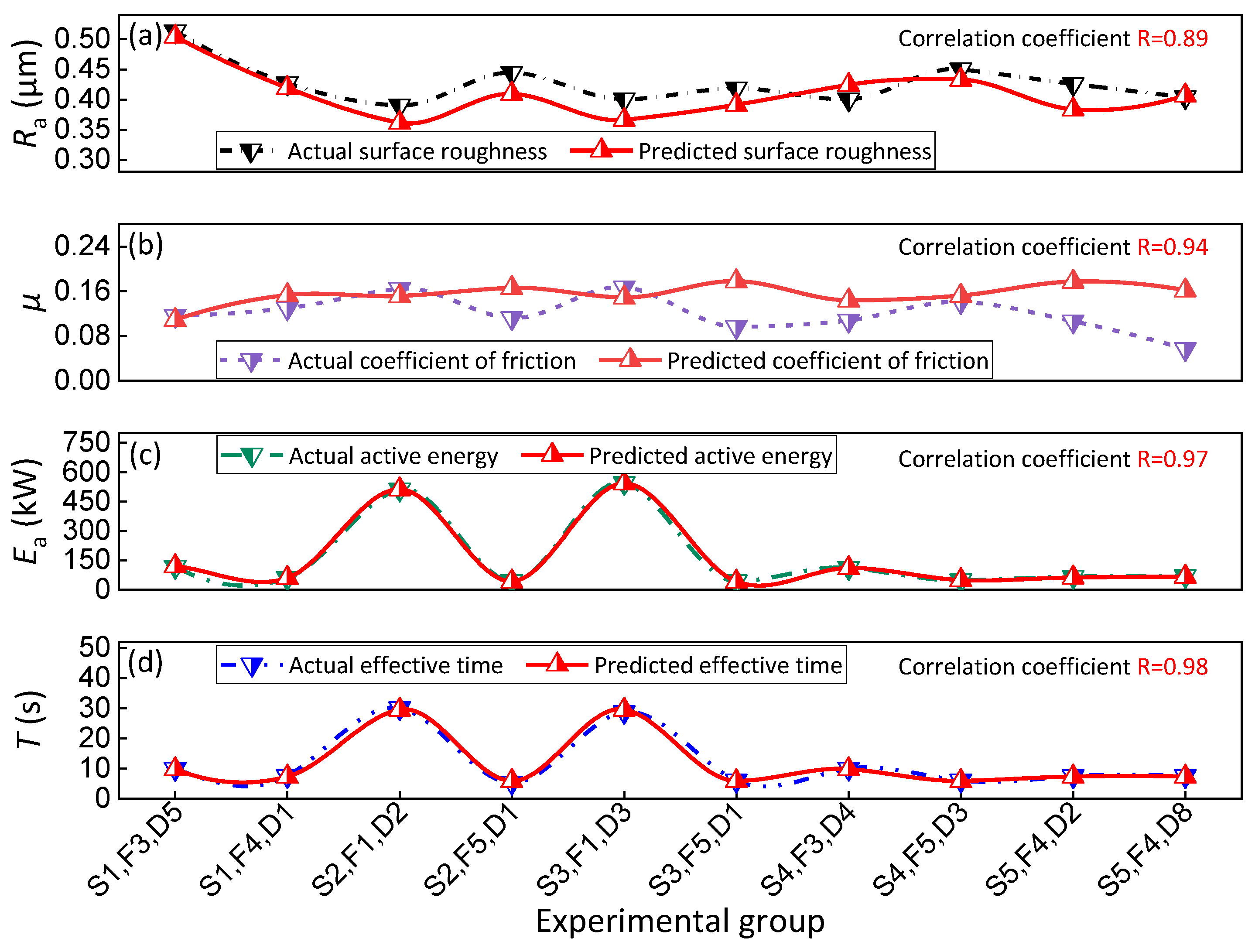
3.3. Mathematical Modeling

In the controllable numerical control range, the different interaction patterns between the evaluation indicators show different expression forms under different processing conditions. Based on the grinding input elements, the output results of surface roughness, coefficient of friction, active energy consumption, and effective grinding time were numerically modeled. Multiple nonlinear regression refers to the unknown independent variables and unknown dependent variables presenting nonlinear characteristics upon regression. Realizing the optimal collocation of multiple independent variables to predict or evaluate dependent variables can improve the validity of the prediction results. In the grinding process, the input parameters and the evaluation results are nonlinear relationships. In this work, a novel method was proposed to judge and identify the function types of independent variables of grinding regarding the grinding evaluation indicators. In order to determine the multivariate nonlinear functional form, logarithms were taken on both sides of functions and transformed into a linear correlation function. The correlation level statistics were then calculated to determine the parameters under the corresponding mathematical mapping model. The parameter was confirmed and numerical modeling was established. The matrix calculation process is shown in Equation (4).

$$\left[\begin{array}{cccc}\lg \delta & {\epsilon }_1& {\epsilon }_2& {\epsilon }_3\\ \lg \eta & {\alpha }_1& {\alpha }_2& {\alpha }_3\\ \lg \gamma & {\beta }_1& {\beta }_2& {\beta }_3\\ \lg \tau & {\rho }_1& {\rho }_2& {\rho }_3\end{array}\right]\left[\begin{array}{c}1\\ \lg v_{\mathrm{s}}\\ \lg v_{\mathrm{w}}\\ \lg v_{\mathrm{p}}\end{array}\right]=\left[\begin{array}{c}\lg R_{\mathrm{a}}\\ \lg u\\ \lg E_{\mathrm{a}}\\ \lg T\end{array}\right]$$

(4)

where the 4 × 4 matrix contains the relevant parameters of each evaluation indicator to be identified. The determination of parameters can be calculated from statistical data and bias regression coefficients by Minitab. Taking 65 groups of grinding experimental data as training samples, the multivariate nonlinear numerical functions of surface roughness R_a, coefficient of friction µ, active energy consumption E_a, and effective grinding time T were constructed. The multivariate nonlinear numerical model of the four evaluation indicators is shown below.

$$R_{\mathrm{a}}=0.8112\cdot v_{\mathrm{s}i}^{-0.2893}\cdot v_{\mathrm{w}i}^{0.1277}\cdot {\alpha }_{\mathrm{p}i}^{0.2014}(i=1,2...65)$$

(5)

$$\mu =0.0114\cdot v_{\mathrm{s}i}^{0.4675}\cdot v_{\mathrm{w}i}^{-0.0236}\cdot {\alpha }_{\mathrm{p}i}^{-0.3164}(i=1,2...65)$$

(6)

$$E_{\mathrm{a}}=18234879\cdot v_{\mathrm{s}i}^{-0.0901}\cdot v_{\mathrm{w}i}^{-1.4878}\cdot {\alpha }_{\mathrm{p}i}^{0.2436}(i=1,2...65)$$

(7)

$$T=30370.3\cdot v_{\mathrm{s}i}^{0.0016}\cdot v_{\mathrm{w}i}^{-1.0054}\cdot {\alpha }_{\mathrm{p}i}^{-0.0004}(i=1,2...65)$$

(8)

Taking the other 10 experimental sets as test samples, the predicted surface roughness, coefficient of friction, active energy consumption, and effective grinding time were compared with the actual evaluation results, as shown in Figure 7.

It can be seen that the predicted results of the established multivariate nonlinear numerical model were in good agreement with the experimental data. The correlation coefficients of surface roughness, coefficient of friction, active energy consumption, and effective grinding time were all high, being 0.89, 0.94, 0.97, and 0.98, respectively. The established numerical model has high reliability and can be used for the following modeling.

3.4. Mathematical Modeling Integration

Based on the multivariate numerical model, an optimized evaluation strategy for grinding-based machining was proposed and constructed to solve a multi-objective optimization problem in this work. In general, a single solution cannot guarantee optimal performance on multiple objectives. And the conflicting nature of the objectives makes it impossible for the algorithm to have a single optimal solution but, instead, a set of relatively good solutions, i.e., Pareto front. The MOEA/D algorithm provides an idea to decompose a multi-objective optimization problem (MOP) into multiple single-objective subproblems through a set of weight vectors. These objectives are optimized simultaneously and each subproblem is optimized by itself using the adjacent population of each subproblem. The algorithm first assigns weight vectors to all individuals randomly generated and uniformly distributed in the population to determine the neighborhood of each subproblem. The subproblem selects individuals in a determined neighborhood for crossover variation to generate new solutions. The individuals of the parent generation in the neighborhood are updated using a specific aggregation function for the next cycle. The best non-dominated individual in each generation is selected and retained as an optimal solution. All optimal solutions are filtered out through continuous iterations of solutions to produce an optimal solution.

An objective function F(x) was established and minimized by considering the following parameters: R_a, μ, E_a, and T. In this study, the number of decision variables was set to be three (v_s, v_w, and a_p), and the number of target variables was four (R_a, μ, E_a, and T). The mathematical description of minimizing MOP under unconstrained conditions can be written as:

$${\{\begin{array}{l}\mathrm{Minimize} \mathrm{F}(x)=\left[R_a(x),\mu (x),E_a(x),T(x)\right]\\ \mathrm{subject} \mathrm{to}:\{\begin{array}{c}1000\le x_1\le 1800\\ 1000\le x_2\le 5000\\ 4\le x_3\le 12\end{array}\end{array}}^{\mathrm{T}}$$

(9)

where x = (x₁, x₂, x₃)∈R³ is a three-dimensional decision variable and F(x)∈R⁴ is a four-dimensional objective variable. The sub-objective function preferences are in order from heavy to light. It is worth noting that the coefficient of friction is a two-level trend. Therefore, the numerical objective function for the coefficient of friction is optimized by seeking the maximum and minimum as an objective for multi-objective optimization.

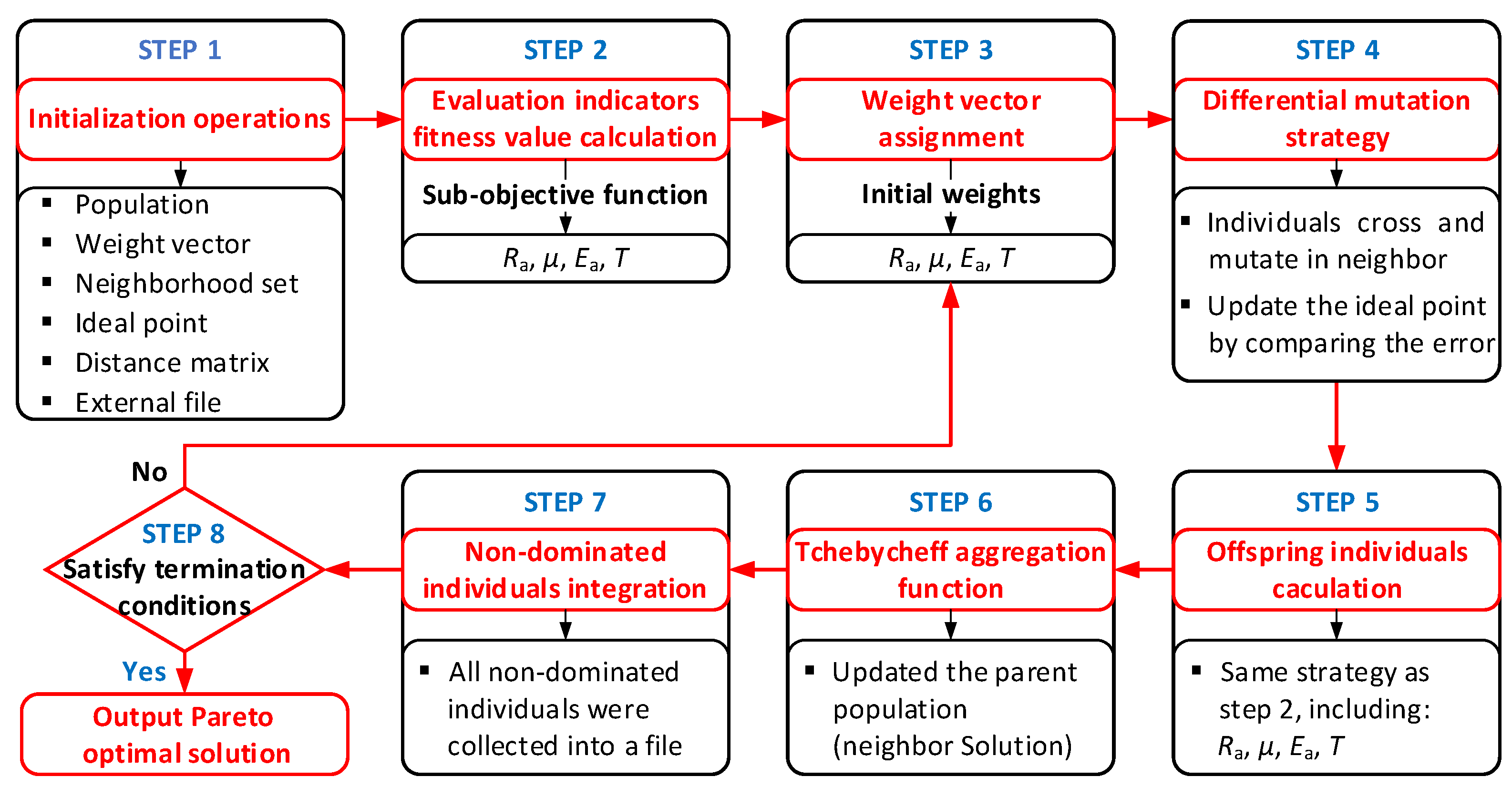
3.4.1. Weight Vector Generation and Aggregation Method for MOEA/D Algorithm

The MOEA/D algorithm uses a simplex lattice point design method to generate the weight vectors of individuals in the population [30]. And it is particularly critical for the algorithm to find an optimal solution, and a relatively uniformly distributed weight vector corresponds to a higher-quality solution. The simplex lattice point design method needs to determine the parameter H (a positive integer) that affects the weight vector. Some uniformly distributed points are selected on the plane composed of w₁ + w₂ +... + w_s =1, where s is the number of objective functions. The generated weight vector requirements are given by

$$w_1^r+w_2^r+\cdot \cdot \cdot w_s^r=1$$

(10)

$$w_i^r\in \left\{\frac{0}{H},\frac{1}{H},\frac{2}{H},\cdot \cdot \cdot \frac{H}{H}\right\},i=1,2,\cdot \cdot \cdot ,sr=1,2,\dots ,N$$

(11)

where H is a parameter that affects the weight vector and is defined by the decision maker, s is the target number/weight vector dimension, w_i^j is the i-th component of the j-th weight vector. The number of population size/weight vectors satisfies the following equation:

$$N=C_{H+S-1}^{S-1}$$

(12)

The generation of weight vectors in MOEA/D algorithm requires the generation of a neighborhood by calculating the Euclidean distance of individuals in the population and the subsequent update of the solution based on the neighboring individuals in the neighborhood. The strategy used to update the solution is to calculate the value of the same aggregation function to retain both solutions on merit. The Tchebycheff approach is a nonlinear multi-objective aggregation method [31] with an aggregation function defined as follows:

$$\{\begin{array}{l}\mathrm{Minimize} g^{\mathrm{TA}}=(x|w,z^{*})=\underset{1\le i\le m}{\max }\left\{w_i\left|{\mathrm{F}}_i(x)-z_i^{*}\right|\right\}\\ \mathrm{subject} \mathrm{to} x\in \mathsf{\Omega }\end{array}$$

(13)

where z* = min{F(x)|x∈Ω}, i∈{1,2, …, s}, w = (w₁,w₂, …, w_m)^T is the weight vector that satisfies w_i ≥ 0. Each solution derived by Equation (13) maps to a Pareto optimal solution x* in the original MOP. The decision maker can choose a different weight vector. When dealing with high-dimensional problems, the TA method can limit the convergence-receiving area and better ensure the convergence of the population.

3.4.2. MOEA/D Algorithm Framework

The MOEA/D algorithm obtains individual neighborhoods by computing the Euclidean distance between the weight vectors of individuals within the population. The relationship between the generated neighborhoods and the subproblems was used to perform simultaneous optimization of the subproblems, so that the individuals within the population keep approximating the ideal Pareto optimal surface. To measure the convergence and distribution of the algorithm, Generational Distance (GD) and Inverted Generational Distance (IGD) were used as evaluation metrics:

$$\mathrm{GD}(P,P^{\ast })=\frac{\sqrt{{\displaystyle {\sum }_{v\in P}{(d(v,p))}^2}}}{\left|P\right|}$$

(14)

$$\mathrm{IGD}(P^{\ast },P)=\frac{{\displaystyle {\sum }_{V\in P^{\ast }}d(v,p)}}{\left|P\right|}$$

(15)

$$d_i={\left\{{\displaystyle {\sum }_{k=1}^s{\left[F_{ki}(x)-F_{k\min }(x)\right]}^2}\right\}}^{1/2}$$

(16)

where P^* is a set of points uniformly distributed over the Pareto front, p is a set of optimal solution sets obtained by the algorithm for approximating the Pareto front, d_i is the i-th individual’s Euclidean distance in this iteration, F_ki(x) is the k-th objective function value of the i-th individual, and F_kmin(x) is the minimum value of the m-th objective function of individuals.

The parent individual selection, the child individual crossover generation, and the population update of the MOEA/D algorithm are all carried out within the neighborhood. This method enables the rapid sharing of good genes with other individuals near the individual, which greatly enhances the search efficiency of the algorithm [32]. The multi-objective optimization strategy flow for the grinding process using the MOEA/D algorithm is shown in Figure 8.

The initial population P₀ satisfying the constraints of size N_p was randomly generated. N_p initial weight vectors w_i^j were generated. The set of neighbors B_i, representing the evolved parent individuals, was selected from d according to the Euclidean distance minimization rule. Then, the ideal point z^* and the empty external file S^* were set. The fitness function values R_a(x), u(x), E_a(x), and T(x) were calculated for the parent individual. All fitness functions were selected as the reciprocal of the sub-objective function. A weight vector was assigned to each sub-objective function. Genetic recombination on individual Xⁱ was then performed as follows: two randomly selected individuals from B_i were cross-mutated to generate new sub-individuals. The ideal point was updated by comparing the ideal point z^* with the objective function value F_r(X^{i, new}) for the offspring individual. All found non-dominated solutions were added to the external file S^* during the evolutionary process. All individuals in S^* that were dominated by new individuals were removed, leaving all solutions in S^* as non-dominated solutions. The stopping criterion was satisfied and the output S^* was used as the Pareto optimal solution set for this optimization problem.

3.5. Optimization Results for the Grinding Process

The parameters set the population size as P0 = 90, the crossover probability as 0.88, the variation probability as 0.07, the maximum number of iterations as 100, and the real-time data update period as 1 s [33]. Based on the above parameter settings, the expert weight values were obtained as (0.64, 0.26, 0.06, 0.04), (0.52, 0.34, 0.09, 0.05), (0.54, 0.15, 0.24, 0.07), and (0.53, 0.20, 0.05, 0.22), respectively. Then, the equation for the coefficient of friction of the sub-function in Equation (6) was maximized and the value of the expert vector obtained was (0.56, 0.36, 0.05, 0.03). The weight ratio of each sub-objective numerical function shows that the surface roughness sub-function has the largest percentage. This indicates surface roughness is crucial in multi-objective optimization. A good sub-objective function indicates a relatively high weight of the objective function. This is consistent with the adversarial nature between sub-objective functions in multi-objective functions.

It is impossible that all indicators satisfy the optimum at the same condition. Based on the weight vector proportion of each sub-function obtained by the MOEA/D algorithm, the genetic algorithm was used to optimize the objective function. The specific parameter settings and process of the genetic algorithm are described in our previous work [34]. The five sets of weight vectors objectively obtained by the MOEA/D algorithm were grouped. The results of the genetic algorithm-optimized grinding elements are listed in order from 1 to 5; see

Table 3. Grinding element optimization results.

Grinding Elements	Weight Vector Grouping Categories
	1	2	3	4	5
vs (m/min)	1560.3760	1638.3838	1753.1953	1765.5965	1724.2324
vw (mm/min)	1094.4094	1033.6033	4708.3708	4647.1647	1286.8286
ap (μm)	4.1712	4.0624	4.3400	4.1208	4.1016

. According to the vector weight grouping category, the three optimized input elements of grinding were brought into Equation (5) in order. The theoretical surface roughness was 0.315 µm, 0.307 µm, 0.370 µm, 0.365 µm, and 0.311 µm. The data analysis reveals that the surface roughness predicted under the premise of minimizing the surface roughness sub-function (the first set of data) is not the minimum. The numerical functions of each sub-objective were brought in turn under the optimized parameter settings as shown in Table 3. The relevant data were obtained as shown in Figure 9. It can be seen that the weight vectors of the third and fourth groups have the best performance in terms of active energy consumption and effective grinding time, respectively. Attributed to the increased proportion of the coefficient of friction sub-function, the weight vectors of the second and fifth groups perform well in terms of surface quality. It is concluded that under the dominance of the surface roughness numerical function, the larger proportion of the numerical function for the coefficient is, the smaller the value of surface roughness from multi-objective optimization is, and the better the surface processing quality is.

Although the weight vectors of the second and fifth groups can achieve better performance, their acquisition paths are based on the minimum and maximum coefficient of friction functions, respectively. The suitable interval for the coefficient of friction obtained by the genetic algorithm was 0.197~0.216, in which the surface roughness was small. The coefficients of friction obtained from the second and fifth sets of optimized parameters are 0.198 and 0.201, respectively. Both can be considered optimal coefficients of friction.

As shown in Figure 9, the surface quality and effective machining time show an opposite trend. This study optimized the weight ratio of surface roughness, coefficient of friction, active energy consumption, and effective grinding time using the MOEA/D algorithm, which was used as the objective function for parameter adjustment. The optimized parameters can greatly reduce the effective machining time under the premise of guaranteeing high grinding surface quality, without the need for repeated process adjustment. The advantage of this method is that the optimal surface finish quality is achieved while minimizing the active energy consumption and the machining time required for that surface quality.

4. Discussion

4.1. Comprehensive Evaluation of Optimization Parameters

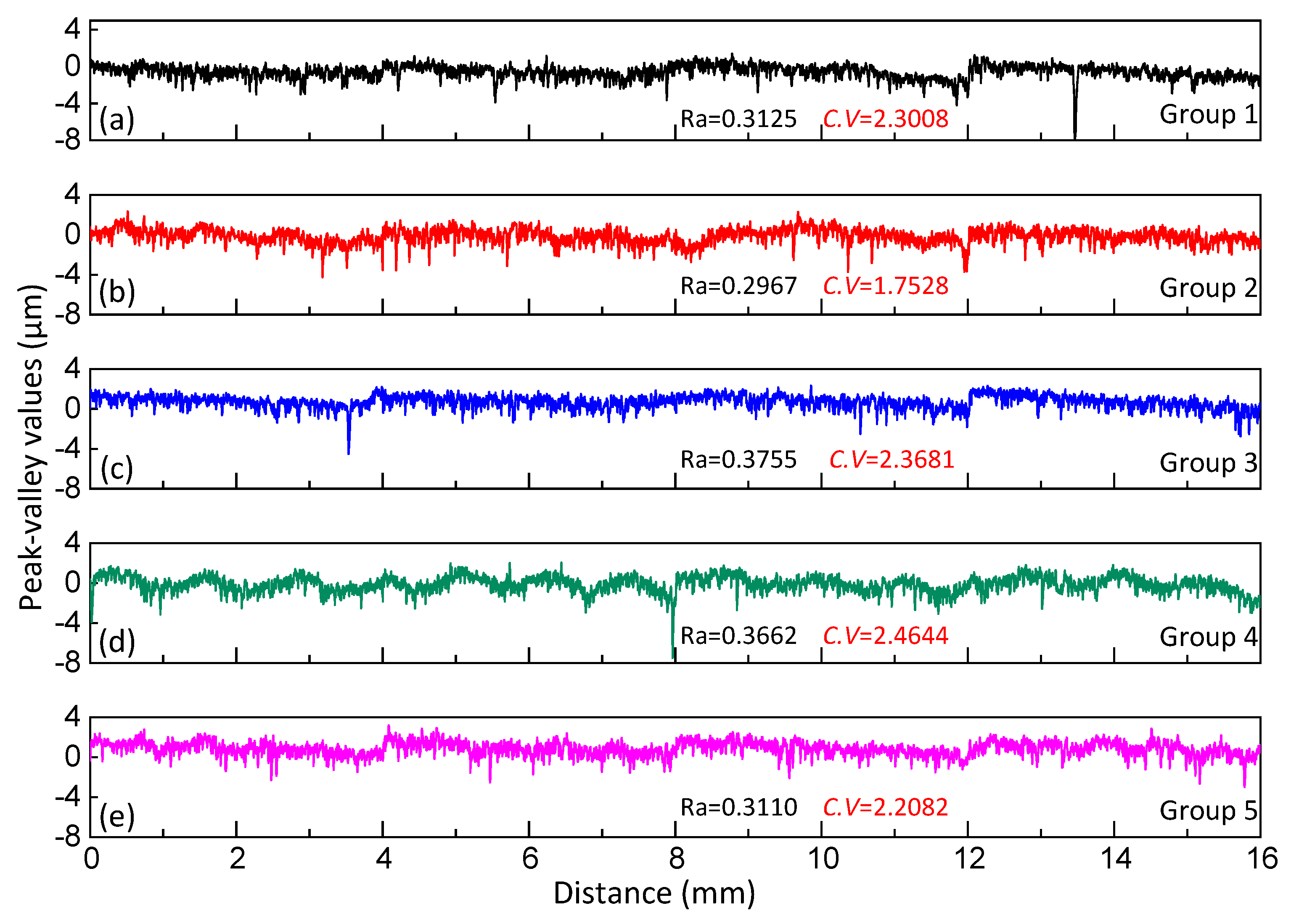
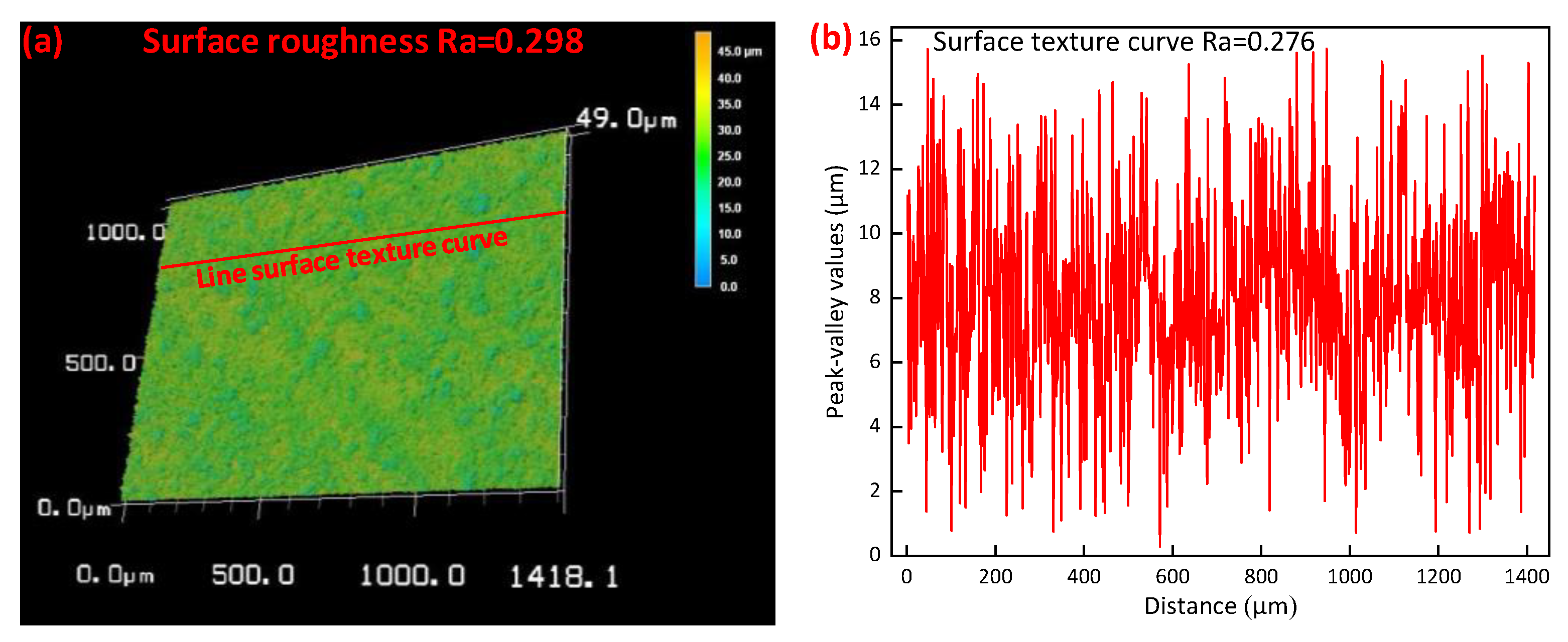
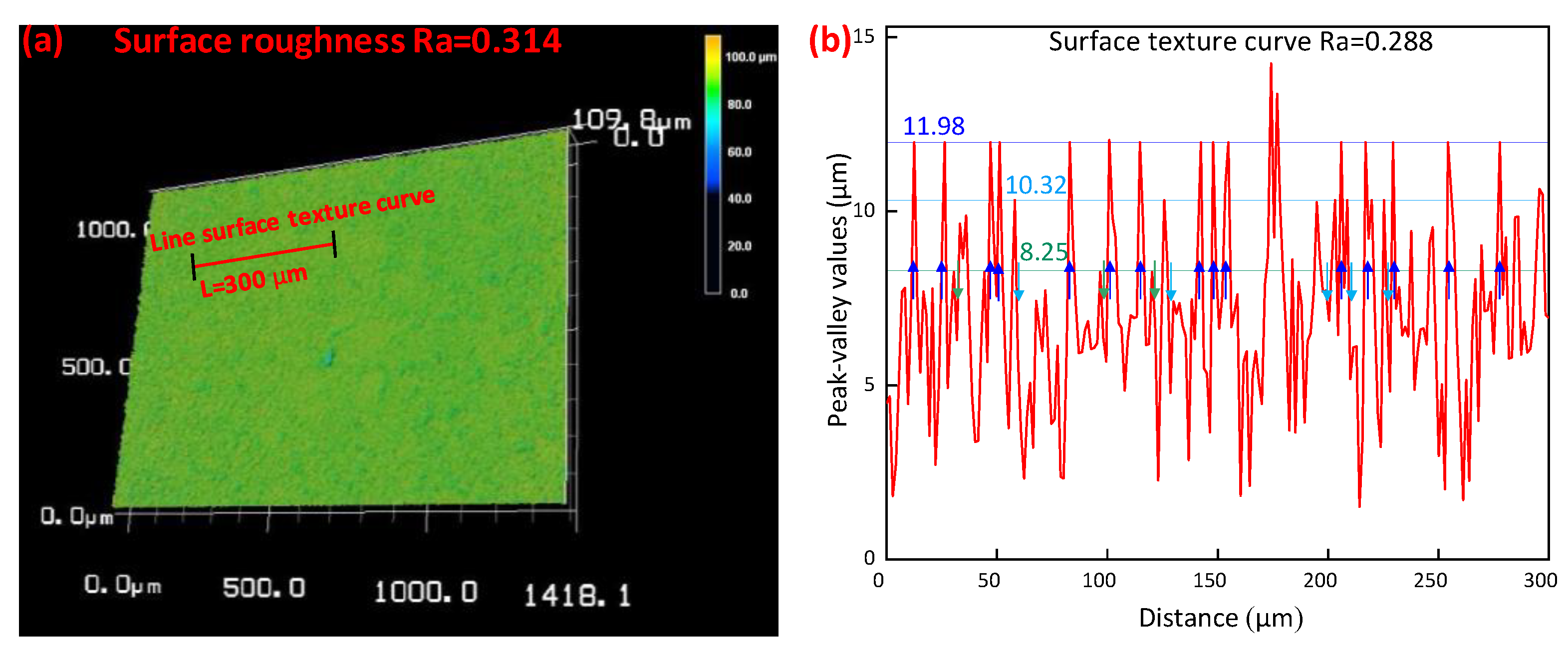
4.1.1. Variation Coefficient and Surface Profile Autocorrelation Analysis

Workpiece surface quality is an important criterion for assessing the grinding process’s performance [35]. Surface roughness is an important parameter of workpiece surface quality [36]. It reflects the unevenness of a machined surface with small spacing and tiny peaks and valleys [37]. Its measurement calculation is an average value determination of least squares. This may lead to a situation where even if the surface roughness is small, the peaks and troughs may differ greatly from the average roughness, indicating poor surface uniformity. So, the idea of a variation coefficient in mathematical statistics is introduced considering the holistic nature of the workpiece. The variation coefficient is used as an evaluation criterion for the degree of data dispersion with the following equation:

$$C.V=(SD/R\mathrm{a})\times 100\%$$

(17)

where SD is the standard deviation of the measurement location.

The coefficient of friction reflects the ratio between the tangential force and the directional force. An appropriate coefficient of friction could make the workpiece surface profile contain both periodic and random components. The surface profile of a workpiece is a very complex random signal [38], and the surface roughness R_a cannot express the full information of its microscopic morphology. Therefore, an autocorrelation analysis of the workpiece surface profile is used for the microscopic analysis of workpiece surface quality [39,40]. The autocorrelation calculation and digital evaluation formula are as follows:

$$R_{xx}(\tau )=\raisebox{1ex}{$1$}\!\left/ \!\raisebox{-1ex}{$D$}\right.{\displaystyle {\int }_0^{D}x(l)}x(l+\tau )dl$$

(18)

where τ is the transverse displacement of the profile curve, D is the evaluation length, and x(l) and x(l + τ) are the contour heights at corresponding coordinates. The autocorrelation function R_xx(τ) is a similarity measure of the workpiece surface profile and usually reaches its maximum value at τ = 0. For a completely random surface profile, R_xx(τ) tends to zero when τ increases gradually. For a periodic profile, the R_xx(τ) curve is also periodic and keeps oscillating steadily as τ increases. For a random surface profile mixed with periodicity, R_xx(τ) gradually decays until it becomes a stable periodic oscillation.

4.1.2. Experimental Verification of Optimized Parameters

Under the same experimental conditions, the optimized machining parameters in Table 3 were used as input to the grinding process. The surface profile, roughness values, and variation coefficient of the workpiece under the above five sets of machining parameters were plotted in Figure 10.

The variation coefficient is calculated from Equation (17). The profile curves are four surface profile curves stitched together. The experimental roughness in Figure 10 has the same change pattern as the predicted roughness values in Figure 9. Both the predicted and experimental values of roughness reach the minimum in the second and fifth groups. The established numerical model accuracy of the multi-objective function is verified. And the distribution uniformity of data points on the surface contour line is verified by the magnitude of the variation coefficient values. It was found that the highest surface quality cannot be achieved when the numerical functions of surface roughness, active energy consumption, or effective grinding time were too dominant. Both the second and the fifth groups achieved the best experimental results using the proportionally superior coefficient of friction’s numerical function. It can be seen that an appropriate coefficient of friction is beneficial to profile uniformity and quality of roughness.

Figure 11 illustrates the uniformity of the data point distribution on the machined surface in terms of both the ceramic surface profile and the line texture curve. Figure 11a shows the 3D shape of the actual machined surface, while Figure 11b shows a surface texture curve. It can be seen from three-dimensional perspectives that the data points of the machined surface have a good uniformity of distribution and the surface machining quality is good. The surface profile roughness value is 0.298 μm and the line roughness value is 0.276 μm.

Autocorrelation function analysis was performed on the experimental grinding surface profile of the workpiece based on the optimized parameter settings. Figure 12 shows the autocorrelation function profile curves for each optimized parameter condition, from which the following rules can be summarized:

Rule 1: The autocorrelation function profiles of the five operating conditions reached the maximum value at τ = 0. The maximum values for the five working conditions were 0.702, 0.561, 0.909, 1.228, and 0.670, respectively. The maximum and minimum values of the autocorrelation coefficient were obtained for the effective machining time-dominated and friction coefficient-dominated operating conditions, respectively. It can be inferred that a smaller effective grinding time indicated a larger longitudinal parameter value of the machined surface and a worse surface quality.

Rule 2: The autocorrelation function curves obtained for all five working conditions decayed with an increase in the horizontal displacement τ. It indicated that there was a randomness signal in all five profile curves. In contrast, the autocorrelation curves of the workpiece surface in the first, third, and fourth groups were smooth and had very few wave fragments. It indicated that there were small periodic signals in the profiles of multi-objective functions dominated by surface roughness, active energy consumption, and effective grinding time. Small periodic signals of the contour curve can also be seen in the case of poor surface quality of the workpiece.

Rule 3: The autocorrelation function of the surface profile had a high-frequency oscillation (the second and fifth groups) in cases where the coefficient of friction’s numerical function was proportionally dominant. The machined surface profile curve has more periodicity components, and the surface quality achieves the best results. It can be demonstrated that the coefficient of friction is important for the periodic variation of microscopic dimensions of the workpiece surface profile.

Figure 13 shows the analysis of the periodic oscillation component of the signal in terms of ceramic surface profile and line texture curves. Figure 13a does not visualize the periodic components, so it is expected that the periodic components are found using the linear surface texture curve. A section of the surface texture curve (length 300 μm) in Figure 13a was selected because too many data points in the line were not conducive to the search for periodic oscillation signals. Figure 13b shows an enlarged view of the linear surface texture profile in Figure 13a. From Figure 13b, it can be seen that there are three levels of periodic oscillation signals (decreasing amplitude, light blue arrow, and blue arrow). The existence of periodic oscillation signals makes the surface obtain better surface quality (Figure 13a can be seen intuitively). The surface profile roughness value and the linear surface texture roughness value are 0.314 μm and 0.288 μm, respectively.

The analysis in this section reveals that the coefficient of friction is related to the roughness of the machined surface. By determining the appropriate coefficient of friction, it is possible to control and regulate the quality of the material production process indicators, to meet the requirements for the use of processed parts and products, which is conducive to the normal production operations of grinding enterprises. When the value for the coefficient of friction is taken between 0.197 and 0.216, the surface roughness of the workpiece is taken between 0.297 μm and 0.311 μm, the value of active energy consumption is taken between 318.769 J and 441.773 J, and effective grinding time is taken between 24.890 s and 30.207 s. The values for the coefficient of friction directly affect the roughness of the machined surface, the active energy consumption, and the effective grinding time, providing important theoretical guidance for the grinding process and providing reference significance for promoting the further development of friction mechanisms.

5. Conclusions

The performance of grinding surfaces directly affects the accuracy, service performance, and surface integrity of workpieces. A multi-objective numerical function was established by fusing and analyzing the collected multi-feature signals, taking into account the surface quality, coefficient of friction, active energy consumption, and effective grinding time. The following conclusions can be drawn:

i.

The four sub-objective function models of surface roughness, coefficient of friction, active energy consumption, and effective grinding time are established with good accuracy. The correlation coefficients of them are high, with values of 0.89, 0.94, 0.97, and 0.98, respectively;

ii.

The weight vectors of sub-objective functions were optimized by the MOEA/D algorithm in the multi-objective numerical function and two sets of optimal weight vectors were obtained. The weight vectors of (R_a, µ, E_a, T) are (0.52, 0.34, 0.09, 0.05) and (0.56, 0.36, 0.05, 0.03). The surface roughness R_a and coefficient of friction µ show a relatively heavy weight;

iii.

Different working parameters were optimized by GA as grinding machine inputs. The optimal input parameters are experimentally verified to be (1638.38 m/min, 1033.60 mm/min, 4.06 μm) and (1724.23 m/min, 1286.83 mm/min, 4.10 μm). The surface roughness, coefficient of friction, active energy consumption, and effective grinding time obtained with the two sets of input parameters are (0.297 μm, 0.199, 441.773 J, 30.207 s) and (0.311 μm, 0.205, 318.769 J, 24.890 s), respectively;

iv.

The coefficient of friction with a range of 0.197~0.216 was beneficial to the surface quality of the workpiece. Whether the friction coefficient tends to 0.197 or 0.216 will produce knowledge of chaos and bifurcation. When the coefficient of friction value tends to be 0.197, the smaller the coefficient of variation of the surface profiles, the smaller the distribution distance deviation of the microscopic data points. The distribution of data points becomes uniform. When it tends to be 0.216, the surface profile shows more periodic characteristics.

References

1. Lin, B.; Wang, H.; Wei, J.; Sui, T. Diamond wheel grinding characteristics of 3D orthogonal quartz fiber reinforced silica ceramic matrix composite. Chin. J. Aeronaut. 2021, 34, 404–414. [Google Scholar] [CrossRef]
2. Xia, L.; Lu, S.; Zhong, B.; Huang, L.; Yang, H.; Zhang, T.; Han, H.; Wang, P.; Xiong, L.; Wen, G. Effect of boron doping on waterproof and dielectric properties of polyborosiloxane coating on SiO2f/SiO2 composites. Chin. J. Aeronaut. 2019, 32, 2017–2027. [Google Scholar] [CrossRef]
3. Dong, W.; Ma, H.; Liu, R.; Liu, T.; Li, S.; Bao, C.; Song, S. Fabrication by stereolithography of fiber-reinforced fused silica composites with reduced crack and improved mechanical properties. Ceram. Int. 2021, 47, 24121–24129. [Google Scholar] [CrossRef]
4. Zheng, Z.; Huang, K.; Lin, C.; Zhang, J.; Wang, K.; Sun, P.; Xu, J. An analytical force and energy model for ductile-brittle transition in ultra-precision grinding of brittle materials. Int. J. Mech. Sci. 2022, 220, 107107. [Google Scholar] [CrossRef]
5. Fernández-Hernán, J.P.; López, A.J.; Torres, B.; Rams, J. Influence of roughness and grinding direction on the thickness and adhesion of sol-gel coatings deposited by dip-coating on AZ31 magnesium substrates. A Landau–Levich equation revision. Surf. Coat. Technol. 2021, 408, 126798. [Google Scholar] [CrossRef]
6. Zhu, S.Y.; Liu, Y.H.; Bai, T.B.; Shi, X.T.; Li, D.M.; Feng, L.B. High-efficient and robust fog collection through topography modulation. Surf. Coat. Technol. 2023, 468, 129747. [Google Scholar] [CrossRef]
7. Qin, R.; Zhang, Z.; Hu, Z.; Du, Z.; Xiang, X.; Wen, G.; He, W. On-line evaluation and monitoring technology for material surface integrity in laser shock peening-A review. J. Mater. Process. Technol. 2023, 313, 117851. [Google Scholar] [CrossRef]
8. Wen, J.R.; Fei, C.W.; Ahn, S.Y.; Han, L.; Huang, B.; Liu, Y.; Kim, H.S. Accelerated damage mechanisms of aluminized superalloy turbine blades regarding combined high-and-low cycle fatigue. Surf. Coat. Technol. 2022, 451, 129048. [Google Scholar] [CrossRef]
9. Wang, S.; Zhao, Q.; Wu, T. An investigation of monitoring the damage mechanism in ultra-precision grinding of monocrystalline silicon based on AE signals processing. J. Manuf. Process. 2022, 81, 945–961. [Google Scholar] [CrossRef]
10. Wang, S.; Sun, G.; Zhao, Q.; Yang, X. Monitoring of ductile-brittle transition mechanisms in sapphire ultra-precision grinding used small grit size grinding wheel through force and acoustic emission signals. Measurement 2023, 210, 112557. [Google Scholar] [CrossRef]
11. Ling, L.G.; Luo, L.; Liu, F.S. Effects of grinding treatment on surface properties and deformation microstructure in alloy 304L. Surf. Coat. Technol. 2021, 408, 126850. [Google Scholar] [CrossRef]
12. Zhang, X.; Chen, H.; Xu, J.; Song, X.; Wang, J.; Chen, X. A novel sound-based belt condition monitoring method for robotic grinding using optimally pruned extreme learning machine. J. Mater. Process. Technol. 2018, 260, 9–19. [Google Scholar] [CrossRef]
13. Tian, Y.B.; Liu, F.; Wang, Y.; Wu, H. Development of portable power monitoring system and grinding analytical tool. J. Manuf. Process. 2017, 27, 188–197. [Google Scholar] [CrossRef]
14. Feng, J.; Kim, B.S.; Shih, A.; Ni, J. Tool wear monitoring for micro-end grinding of ceramic materials. J. Mater. Process. Technol. 2009, 209, 5110–5116. [Google Scholar] [CrossRef]
15. Qin, F.; Zhang, L.X.; Chen, P.; An, T.; Dai, Y.W.; Gong, Y.P.; Yi, Z.B.; Wang, H.M. In situ wireless measurement of grinding force in silicon wafer self-rotating grinding process. Mech. Syst. Signal Process. 2021, 154, 107550. [Google Scholar] [CrossRef]
16. Warren, T.L.; Ting, C.; Qu, J.; Blau, P.J. A wavelet-based methodology for grinding wheel condition monitoring. Int. J. Mach. Tools Manuf. 2007, 47, 580–592. [Google Scholar] [CrossRef]
17. Ma, L.; Gong, Y.; Chen, X. Study on surface roughness model and surface forming mechanism of ceramics in quick point grinding. Int. J. Mach. Tools Manuf. 2014, 77, 82–92. [Google Scholar] [CrossRef]
18. Yao, Z.; Gu, W.; Li, K. Relationship between surface roughness and subsurface crack depth during grinding of optical glass BK7. J. Mater. Process. Technol. 2012, 212, 969–976. [Google Scholar] [CrossRef]
19. Kong, D.D.; Zhu, J.J.; Duan, C.Q.; Lu, L.X.; Chen, D.X. Bayesian linear regression for surface roughness prediction. Mech. Syst. Signal Process. 2020, 142, 106770. [Google Scholar] [CrossRef]
20. Meng, Q.; Guo, B.; Wu, G.; Xiang, Y.; Guo, Z.; Jia, J.; Zhao, Q.; Li, K.; Zeng, Z. Dynamic force modeling and mechanics analysis of precision grinding with microstructured wheels. J. Mater. Process. Technol. 2023, 314, 117900. [Google Scholar] [CrossRef]
21. Lei, X.; Xiang, D.; Peng, P.; Liu, G.; Li, B.; Zhao, B.; Gao, G. Establishment of dynamic grinding force model for ultrasonic-assisted single abrasive high-speed grinding. J. Mater. Process. Technol. 2022, 300, 117420. [Google Scholar] [CrossRef]
22. Liu, R.; Yang, B.; Zio, E.; Chen, X. Artificial intelligence for fault diagnosis of rotating machinery: A review. Mech. Syst. Signal Process. 2018, 108, 33–47. [Google Scholar] [CrossRef]
23. Dai, C.; Ding, W.; Zhu, Y.; Xu, J.; Yu, H. Grinding temperature and power consumption in high speed grinding of Inconel 718 nickel-based superalloy with a vitrified CBN wheel. Precis. Eng. 2018, 52, 192–200. [Google Scholar] [CrossRef]
24. Wang, J.L.; Tian, Y.B.; Hu, X.T.; Li, Y.; Zhang, K.; Liu, Y.H. Predictive modelling and Pareto optimization for energy efficient grinding based on aANN-embedded NSGA II algorithm. J. Clean. Prod. 2021, 327, 129479. [Google Scholar] [CrossRef]
25. Wang, J.L.; Tian, Y.B.; Zhang, K.; Liu, Y.H.; Cong, J.C. Online prediction of grinding wheel condition and surface roughness for the fused silica ceramic composite material based on the monitored power signal. J. Mater. Res. Technol. 2023, 24, 8053–8064. [Google Scholar] [CrossRef]
26. Li, Y.; Liu, Y.H.; Wang, J.L.; Wang, Y.; Tian, Y.B. Real-time monitoring of silica ceramic composites grinding surface roughness based on signal spectrum analysis. Ceram. Int. 2022, 48, 7204–7217. [Google Scholar] [CrossRef]
27. Wang, J.L.; Li, J.W.; Tian, Y.B.; Liu, Y.H.; Zhang, K. Methods of grinding power signal acquisition and dynamic power monitoring database establishment. Diam. Abras. Eng. 2022, 42, 356–363. [Google Scholar] [CrossRef]
28. Zhang, K.; Tian, Y.B.; Cong, J.C.; Liu, Y.H.; Yan, N.; Lu, T. Reduction grinding energy consumption by modified particle swarm optimization based on dynamic inertia weigh. Diam. Abras. Eng. 2020, 41, 71–75. [Google Scholar] [CrossRef]
29. Wang, J.L.; Tian, Y.B.; Hu, X.T.; Han, J.G.; Liu, B. Integrated assessment and optimization of dual environment and production drivers in grinding. Energy 2023, 272, 127046. [Google Scholar] [CrossRef]
30. Zhang, Q.; Li, H. MOEA/D: A Multiobjective Evolutionary Algorithm Based on Decomposition. IEEE Trans. Evol. Comput. 2008, 11, 712–731. [Google Scholar] [CrossRef]
31. Jaszkiewicz, A. On the performance of multiple-objective genetic local search on the 0/1 knapsack problem-a comparative experiment. IEEE Trans. Evol. Comput. 2000, 6, 402–412. [Google Scholar] [CrossRef]
32. Wang, W.; Li, K.; Tao, X.; Gu, F. An improved MOEA/D algorithm with an adaptive evolutionary strategy. Inf. Sci. 2020, 539, 1–15. [Google Scholar] [CrossRef]
33. Qin, S.; Sun, C.; Zhang, G.; He, X.; Tan, Y. A modified particle swarm optimization based on decomposition with different ideal points for many-objective optimization problems. Complex Intell. Syst. 2020, 6, 263–274. [Google Scholar] [CrossRef]
34. Li, Y.; Liu, Y.H.; Tian, Y.B.; Wang, Y.; Wang, J.L. Application of improved fireworks algorithm in grinding surface roughness online monitoring. J. Manuf. Process. 2022, 74, 400–412. [Google Scholar] [CrossRef]
35. Jiang, J.; Ge, P.; Hong, J. Study on micro-interacting mechanism modeling in grinding process and ground surface roughness prediction. Int. J. Adv. Manuf. Technol. 2013, 67, 1035–1052. [Google Scholar] [CrossRef]
36. Wang, Q.; Cong, W.; Pei, Z.J.; Gao, H.; Kang, R. Rotary ultrasonic machining of potassium dihydrogen phosphate (KDP) crystal: An experimental investigation on surface roughness. J. Manuf. Process. 2009, 11, 66–73. [Google Scholar] [CrossRef]
37. Zhang, Y.; Li, C.; Jia, D.; Li, B.; Wang, Y.; Yang, M.; Hou, Y.; Zhang, X. Experimental study on the effect of nanoparticle concentration on the lubricating property of nanofluids for MQL grinding of Ni-based alloy. J. Mater. Process. Technol. 2016, 232, 100–115. [Google Scholar] [CrossRef]
38. Jiang, J.L.; Ge, P.Q.; Bi, W.B.; Zhang, L.; Wang, D.X.; Zhang, Y. 2D/3D ground surface topography modeling considering dressing and wear effects in grinding process. Int. J. Mach. Tools Manuf. 2013, 74, 29–40. [Google Scholar] [CrossRef]
39. Zhang, X.; Li, C.; Zhang, Y.; Wang, Y.; Li, B.; Yang, M.; Guo, S.; Liu, G.; Zhang, N. Lubricating property of MQL grinding of Al2O3/SiC mixed nanofluid with different particle sizes and microtopography analysis by cross-correlation. Precis. Eng. 2017, 47, 532–545. [Google Scholar] [CrossRef]
40. Zhang, X.; Li, C.; Zhang, Y.; Jia, D.; Li, B.; Wang, Y.; Yang, M.; Hou, Y.; Zhang, X. Performances of Al2O3/SiC hybrid nanofluids in minimum-quantity lubrication grinding. Int. J. Adv. Manuf. Technol. 2016, 86, 3427–3441. [Google Scholar] [CrossRef]
Figure 1. Grinding test configuration and data measurement.
Lubricants 11 00351 g001
Figure 2. The processing method of grinding force signals (vs = 1000 m/min, vw = 1000 mm/min, ap = 10 μm).
Lubricants 11 00351 g002
Figure 3. The processing method of grinding power signals (vs = 1000 m/min, vw = 3000 mm/min, ap = 12 μm).
Lubricants 11 00351 g003
Figure 4. The relationship between coefficient of friction and surface roughness.
Lubricants 11 00351 g004
Figure 5. The relationship between active energy consumption and surface roughness.
Lubricants 11 00351 g005
Figure 6. The relationship between effective grinding time and surface roughness.
Lubricants 11 00351 g006
Figure 7. Validity verification of numerical model. (a) Validation of the surface roughness numerical model. (b) Validation of the coefficient of friction numerical model. (c) Validation of the active energy consumption numerical model. (d) Validation of the effective grinding time numerical model.
Lubricants 11 00351 g007
Figure 8. MOEA/D algorithm multi-objective optimization process.
Lubricants 11 00351 g008
Figure 9. Sub-objective function values based on optimized parameters.
Lubricants 11 00351 g009
Figure 10. Surface profile curve, surface roughness, and variation coefficient. (a) Experimental results under optimized parameter 1 (vs = 1560.3760 m/min, vw = 1094.4094 mm/min, ap = 4.1712 μm). (b) Experimental results under optimized parameter 2 (vs = 1638.3838 m/min, vw = 1033.6033 mm/min, ap = 4.0624 μm). (c) Experimental results under optimized parameter 3 (vs = 1753.1953 m/min, vw = 4708.3708 mm/min, ap = 4.3400 μm). (d) Experimental results under optimized parameter 4 (vs = 1765.5965 m/min, vw = 4647.1647 mm/min, ap = 4.1208 μm). (e) Experimental results under optimized parameter 5 (vs = 1724.2324 m/min, vw = 1286.8286 mm/min, ap = 4.1016 μm).
Lubricants 11 00351 g010
Figure 11. Ceramic surface profile and line texture curve (vs = 1638.38 m/min, vw = 1033.60 mm/min, ap = 4.06 μm). (a) 3D topography of the machined surface. (b) Surface texture peak-to-valley curve.
Lubricants 11 00351 g011
Figure 12. Surface profile autocorrelation function curves under multivariate optimization parameters. (a) Autocorrelation function curve under optimized parameter 1 (vs = 1560.3760 m/min, vw = 1094.4094 mm/min, ap = 4.1712 μm). (b) Autocorrelation function curve under optimized parameter 2 (vs = 1638.3838 m/min, vw = 1033.6033 mm/min, ap = 4.0624 μm). (c) Autocorrelation function curve under optimized parameter 3 (vs = 1753.1953 m/min, vw = 4708.3708 mm/min, ap = 4.3400 μm). (d) Autocorrelation function curve under optimized parameter 4 (vs = 1765.5965 m/min, vw = 4647.1647 mm/min, ap = 4.1208 μm). (e) Autocorrelation function curve under optimized parameter 5 (vs = 1724.2324 m/min, vw = 1286.8286 mm/min, ap = 4.1016 μm).
Lubricants 11 00351 g012
Figure 13. Ceramic surface profile and linear texture curve (vs = 1724.23 m/min, vw = 1286.83 mm/min, ap = 4.10 μm). (a) 3D topography of the machined surface. (b) Surface texture peak-to-valley curve.
Lubricants 11 00351 g013