Extrapolation of Hydrodynamic Pressure in Lubricated Contacts: A Novel Multi-Case Physics-Informed Neural Network Framework

 , , , , and
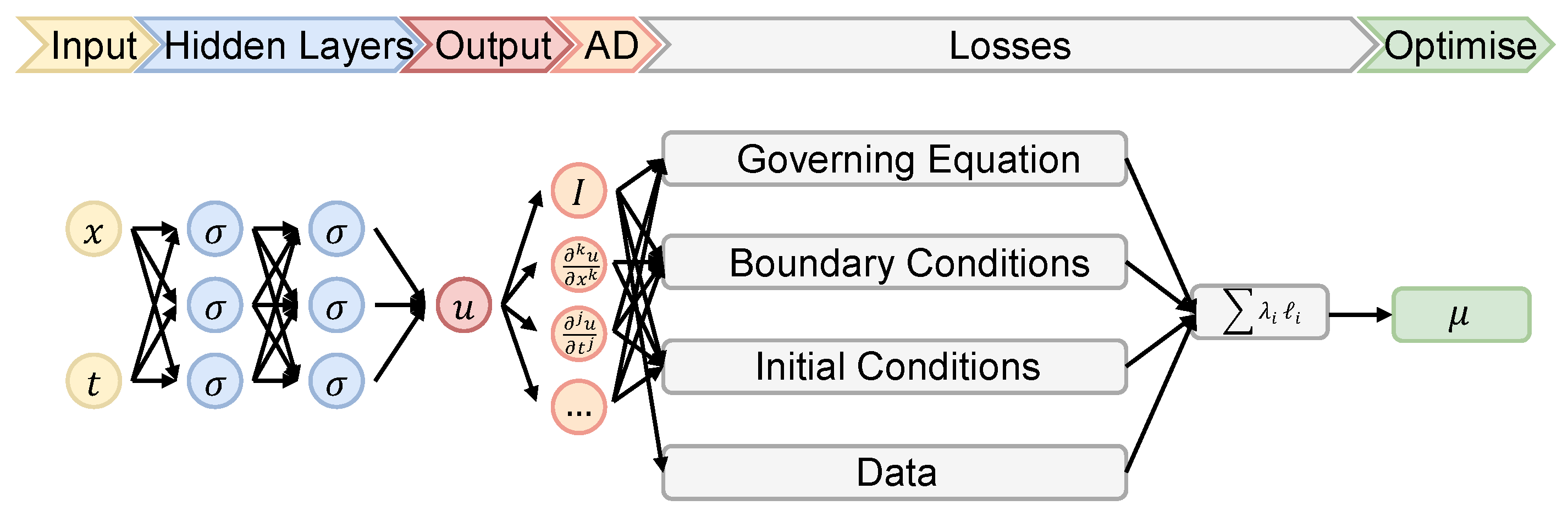
Abstract
:1. Introduction
2. Materials and Methods
2.1. Hydrodynamic Lubrication
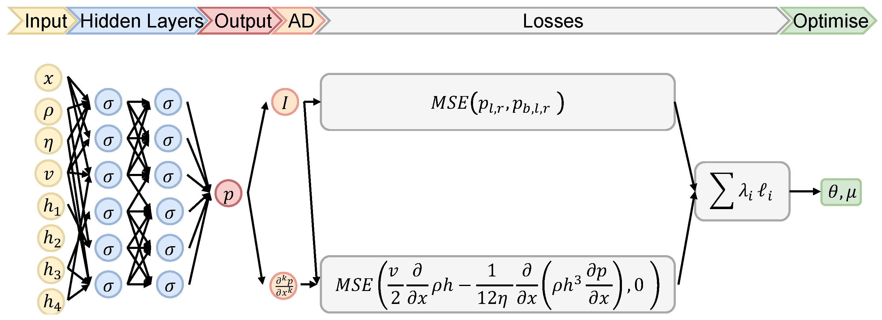
2.2. Physics-Informed Neural Networks
2.2.1. Physical-Informed Loss
- (no cavitation)
- , (ideally smooth surface)
- (incompressible)
- Stationary: Partial derivatives with respect to time are irrelevant
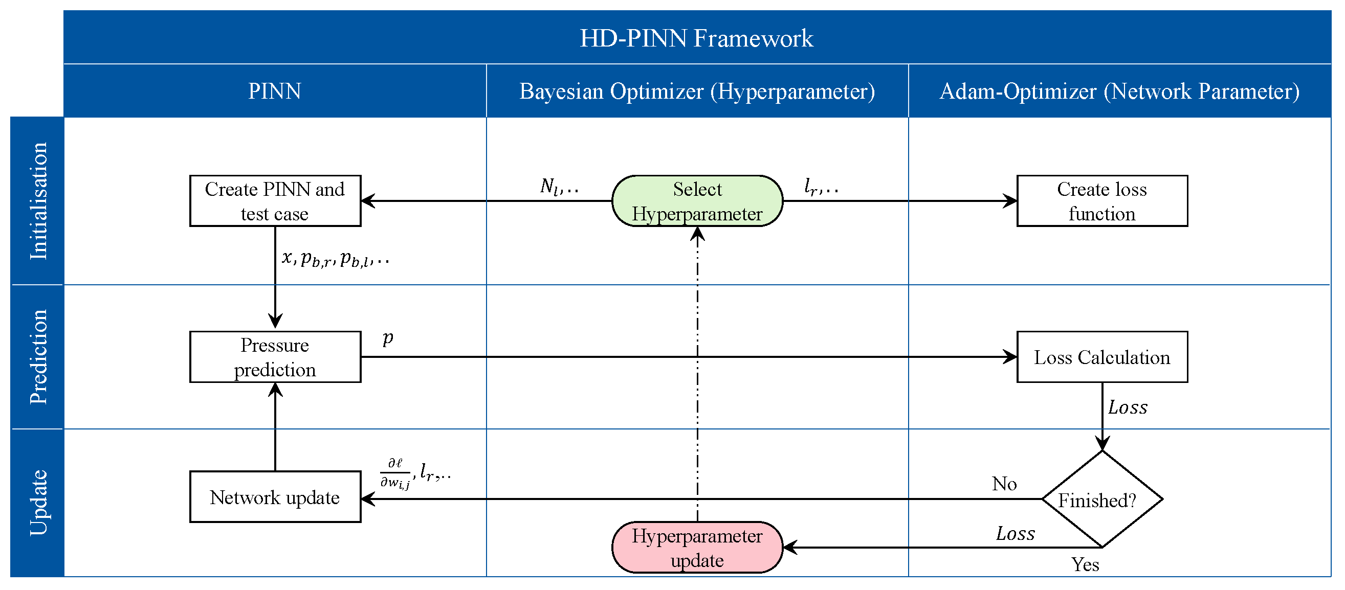
2.3. HD-PINN Framework
2.4. Test Cases
- The height multi-case analysis involved a linear convergent profile, where the parameter varied within the range from to , holding constant at , and the pressure boundaries and were set to and , respectively.
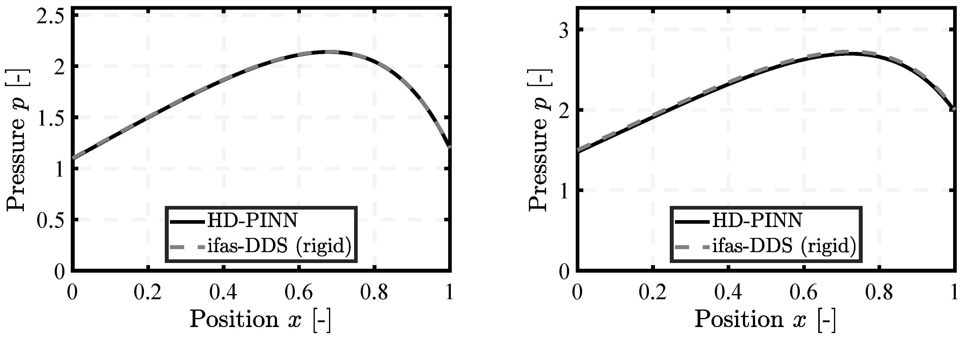
- For the pressure boundary multi-case scenarios, a linear convergent profile was considered with both and varying across the range from 0 to 1.
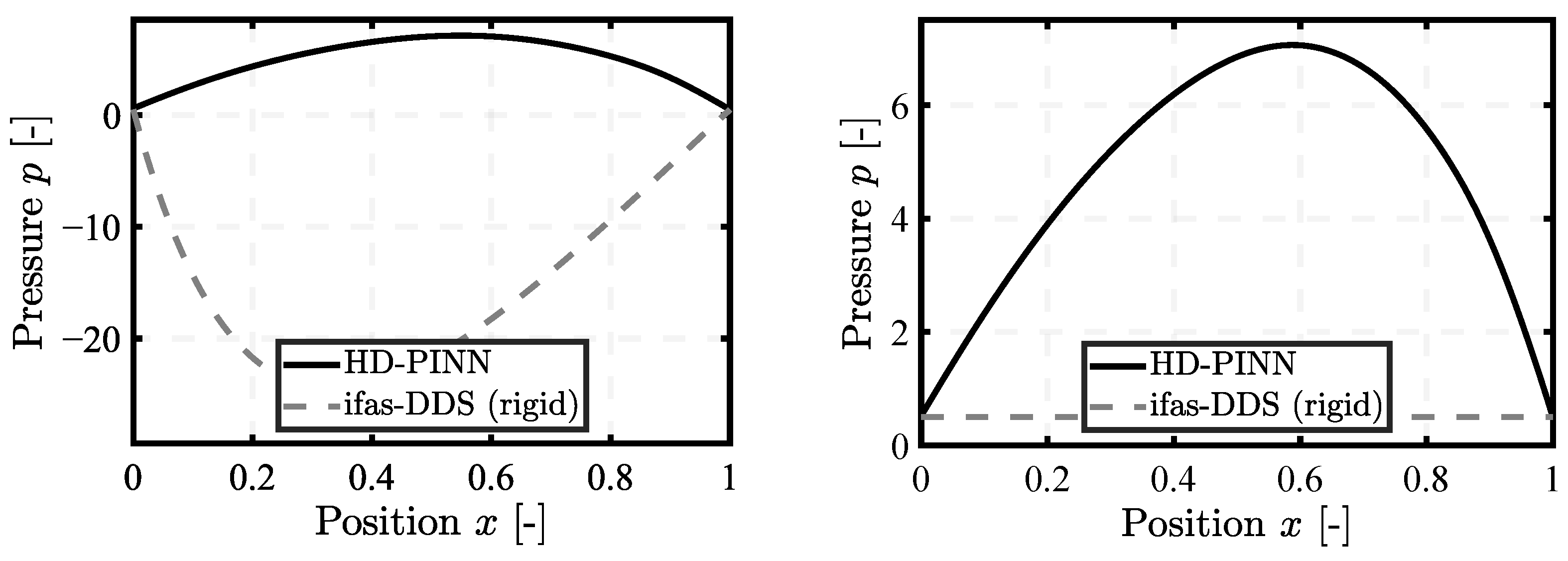
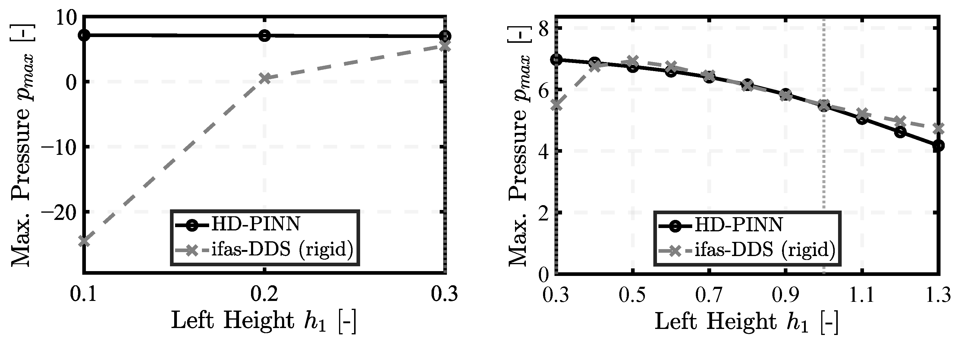
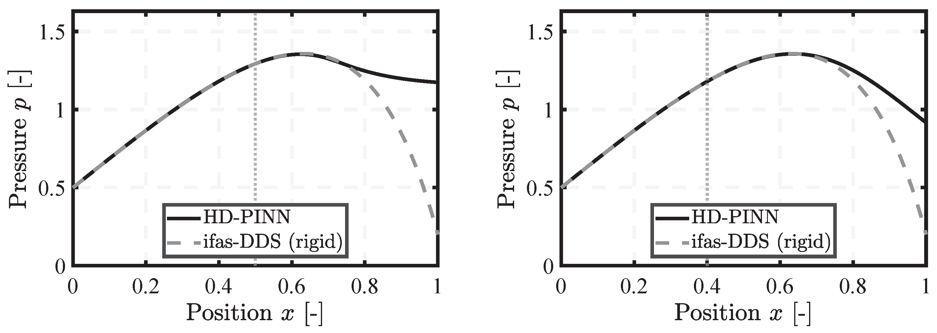
- Height extrapolation tasks were extended beyond the original multi-case domain for , exploring values from down to and up from to .
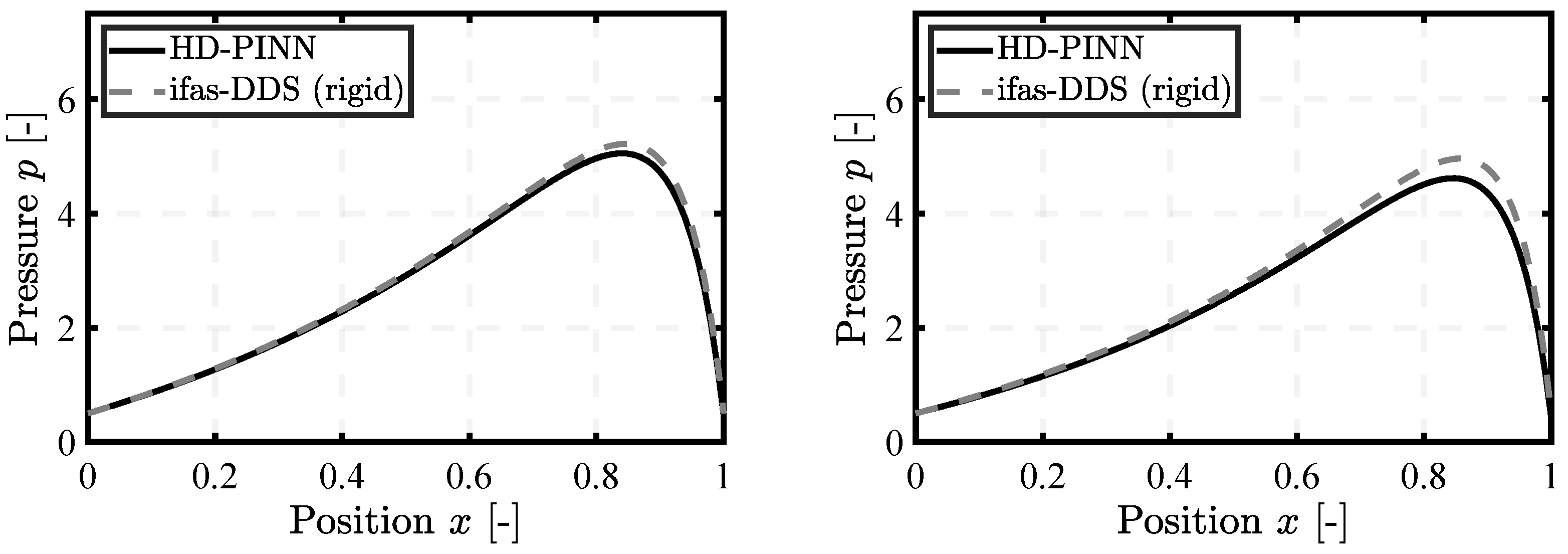
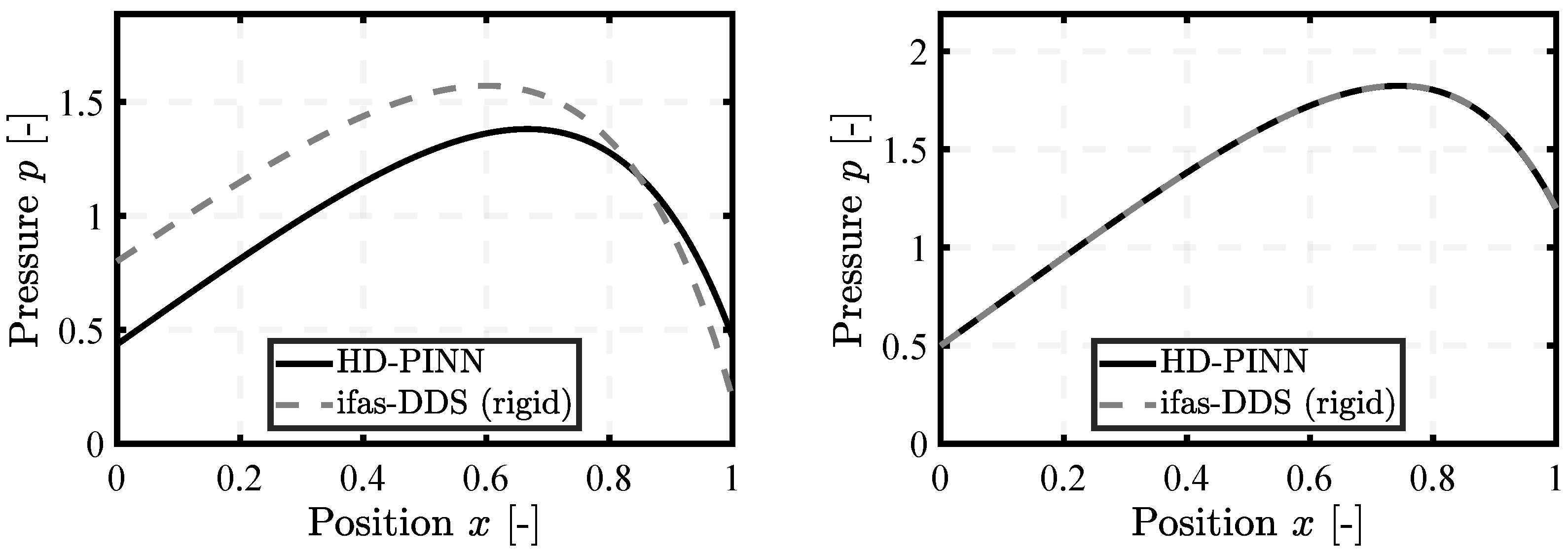
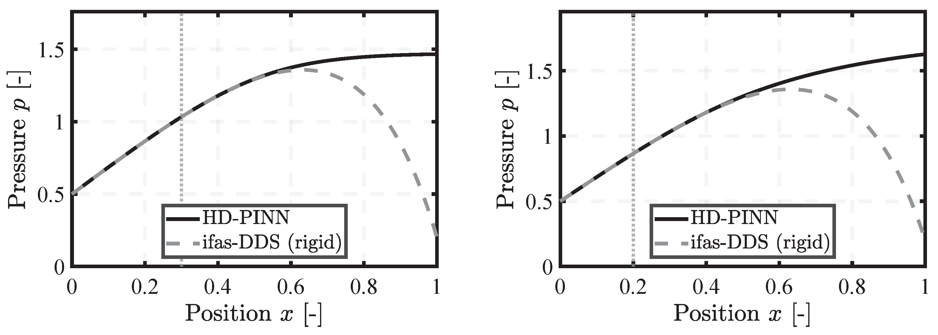
- Pressure boundary extrapolation tested the PINN with scenarios outside the multi-case training domain, specifically for pressure boundary combinations of , , and .
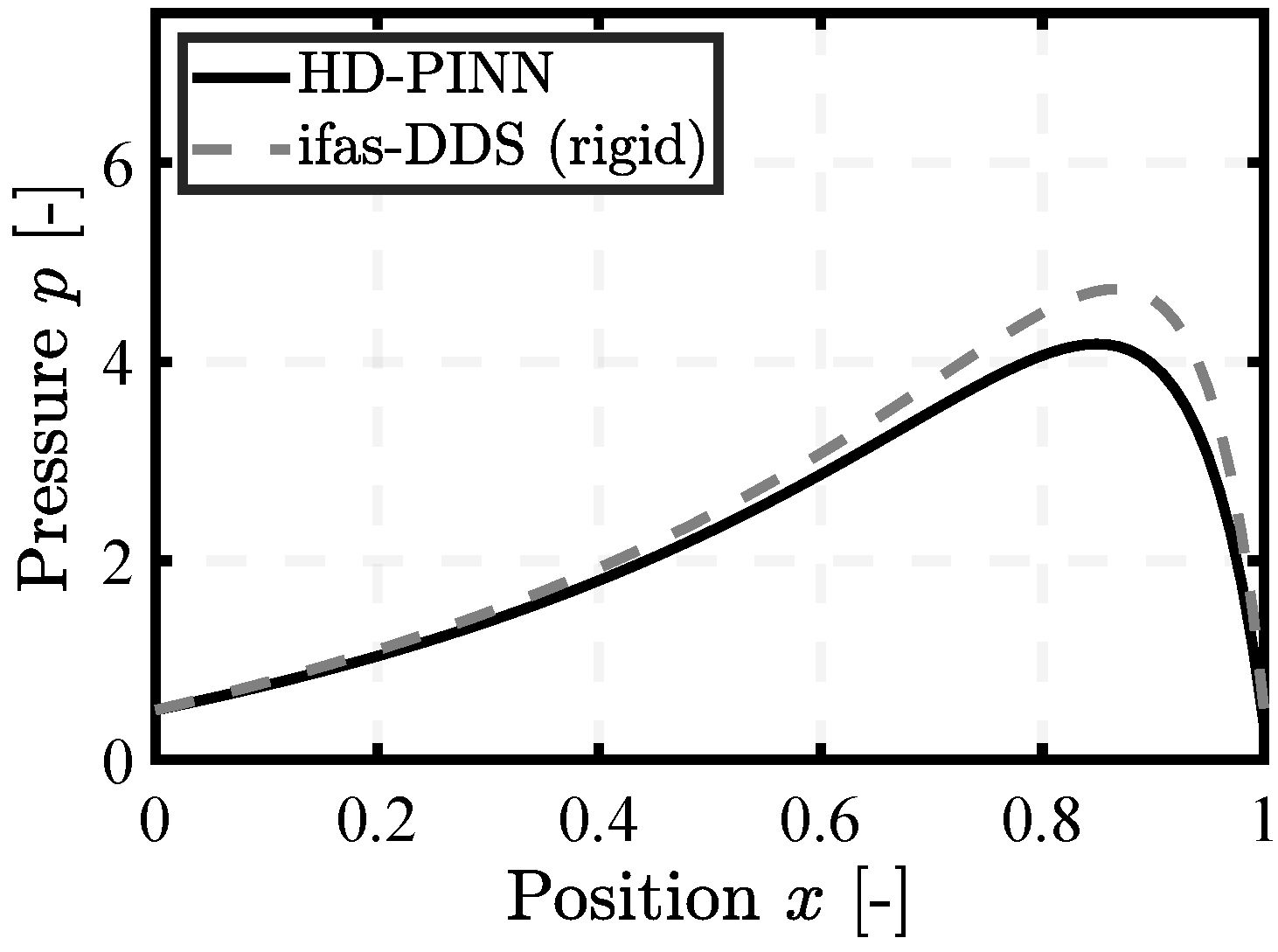
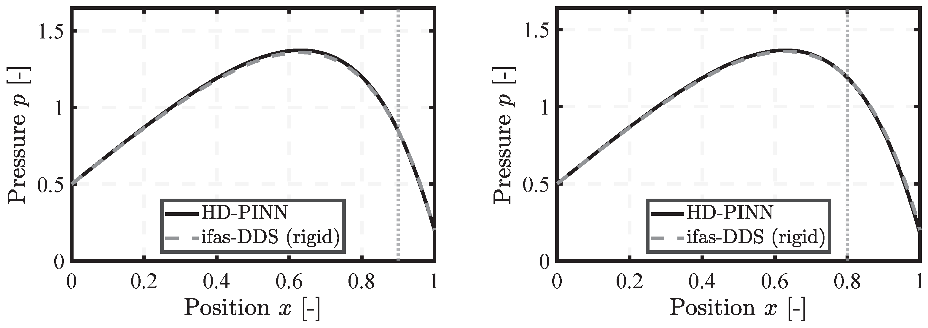
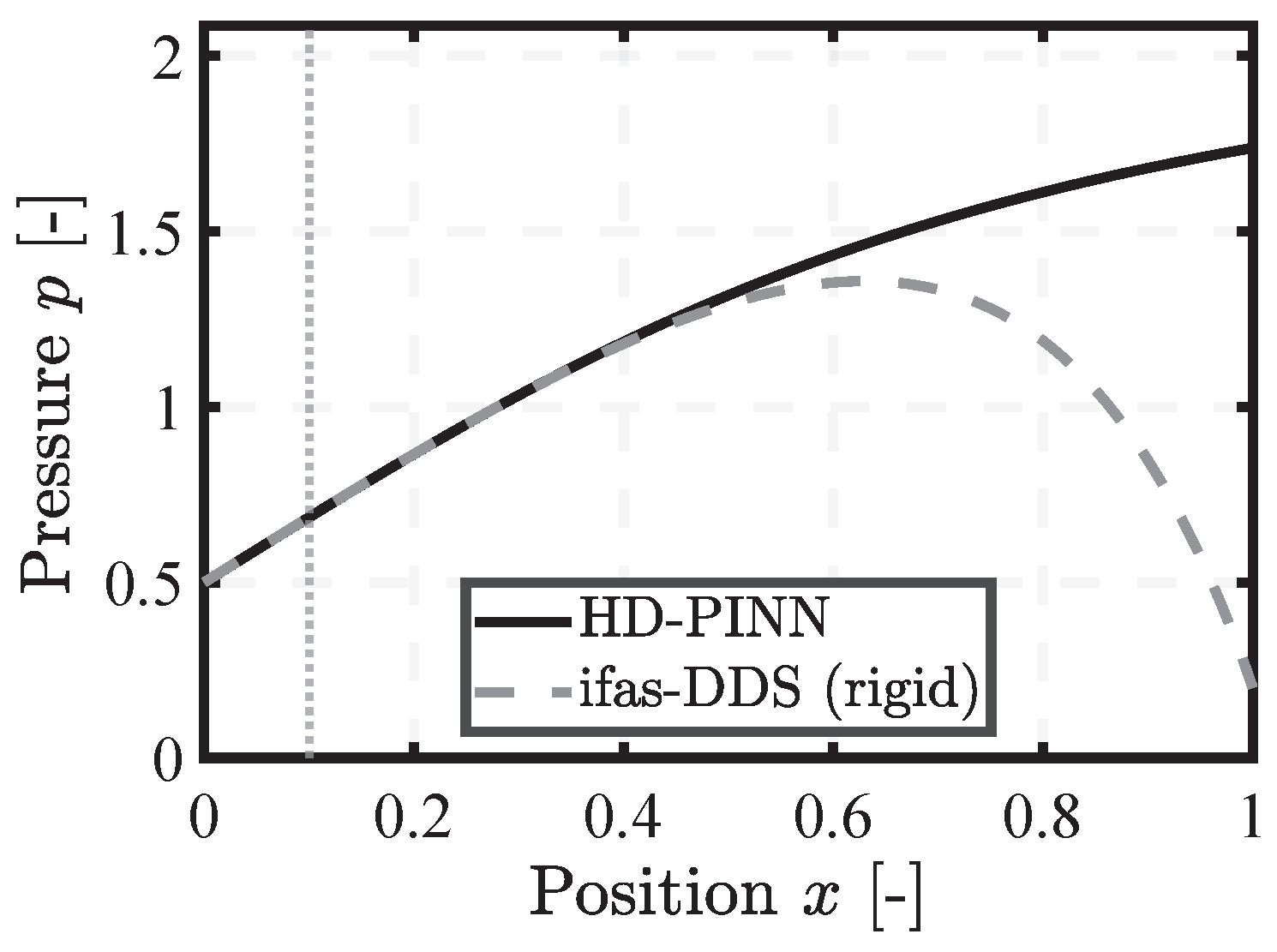
- Position extrapolation was investigated for a linear convergent height profile with fixed pressure boundaries , where the right boundary position varied from down to .
3. Results
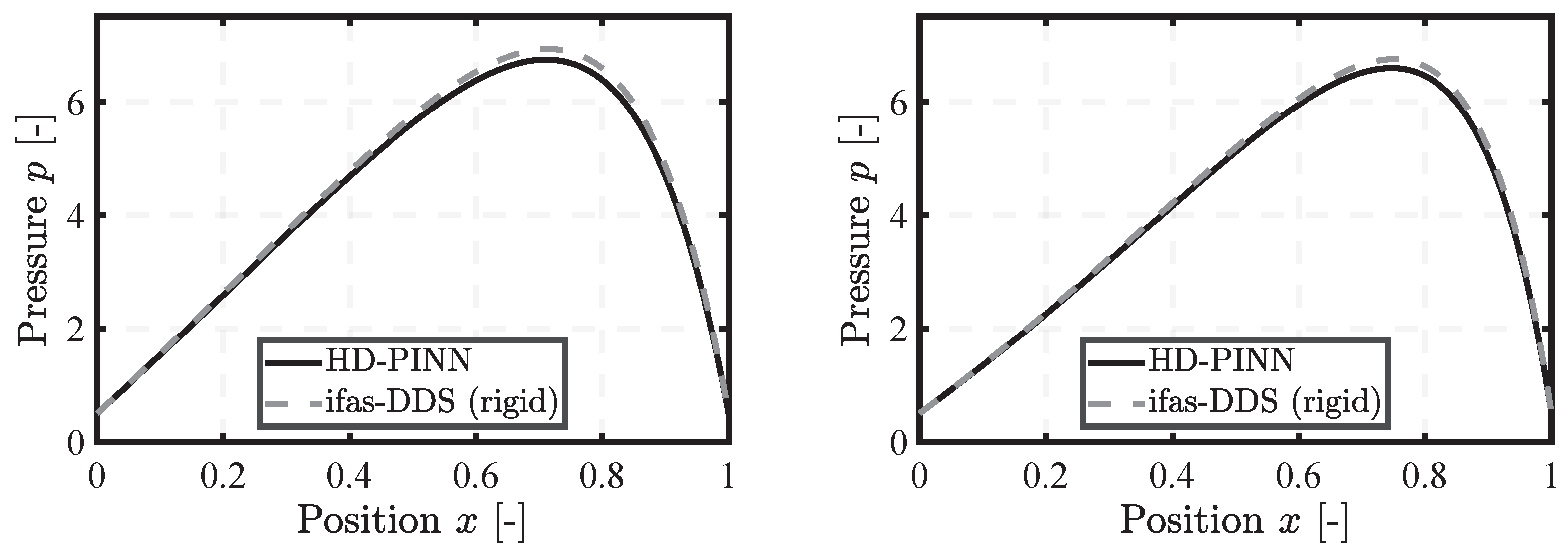
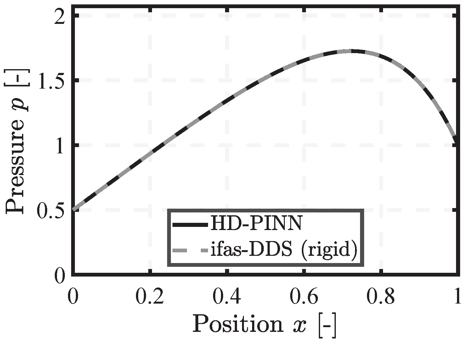
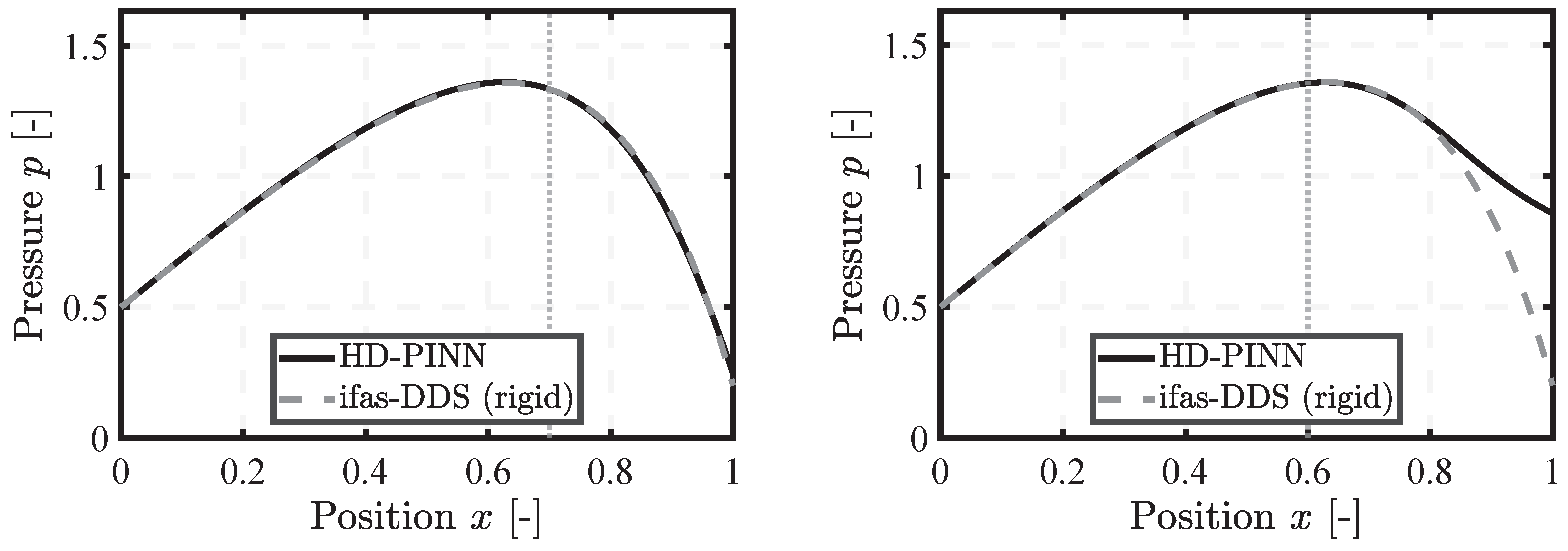
3.1. Height Multi-Case
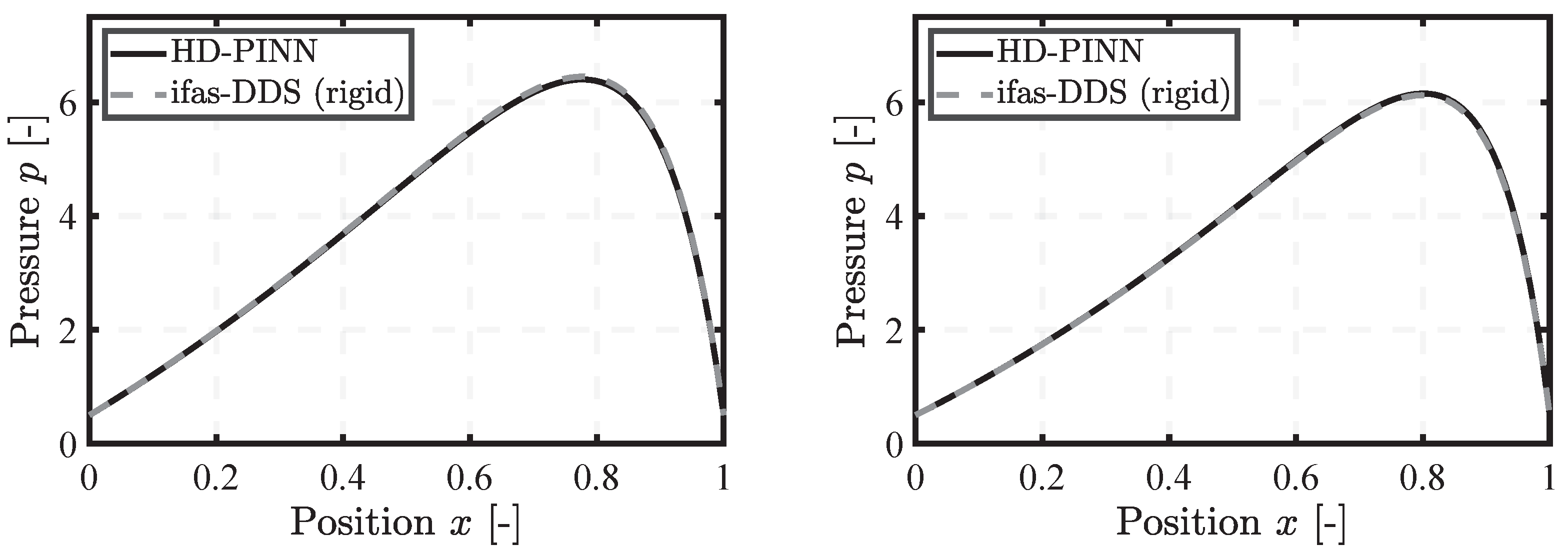
3.2. Pressure Boundary Multi-Case
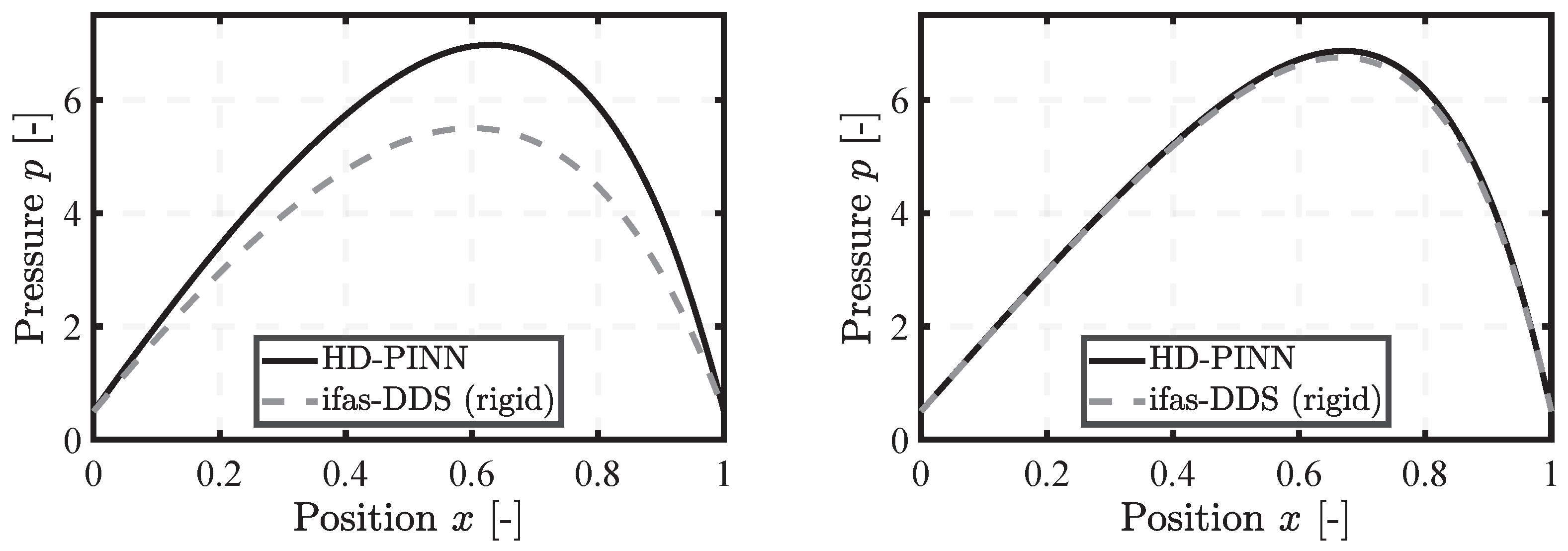
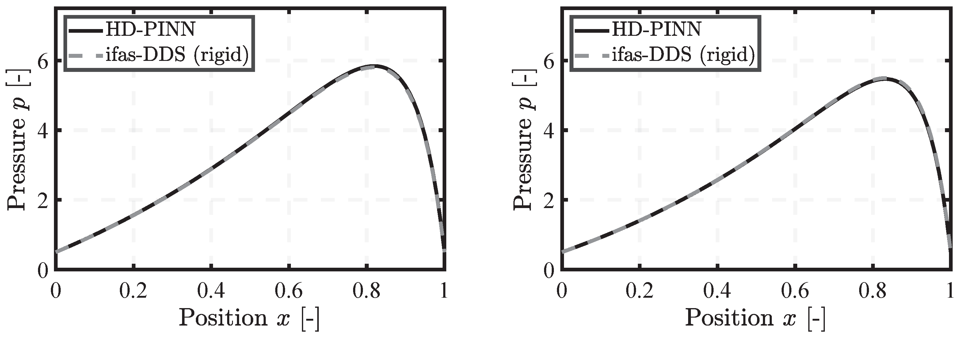
3.3. Height Extrapolation
3.4. Pressure Boundary Extrapolation
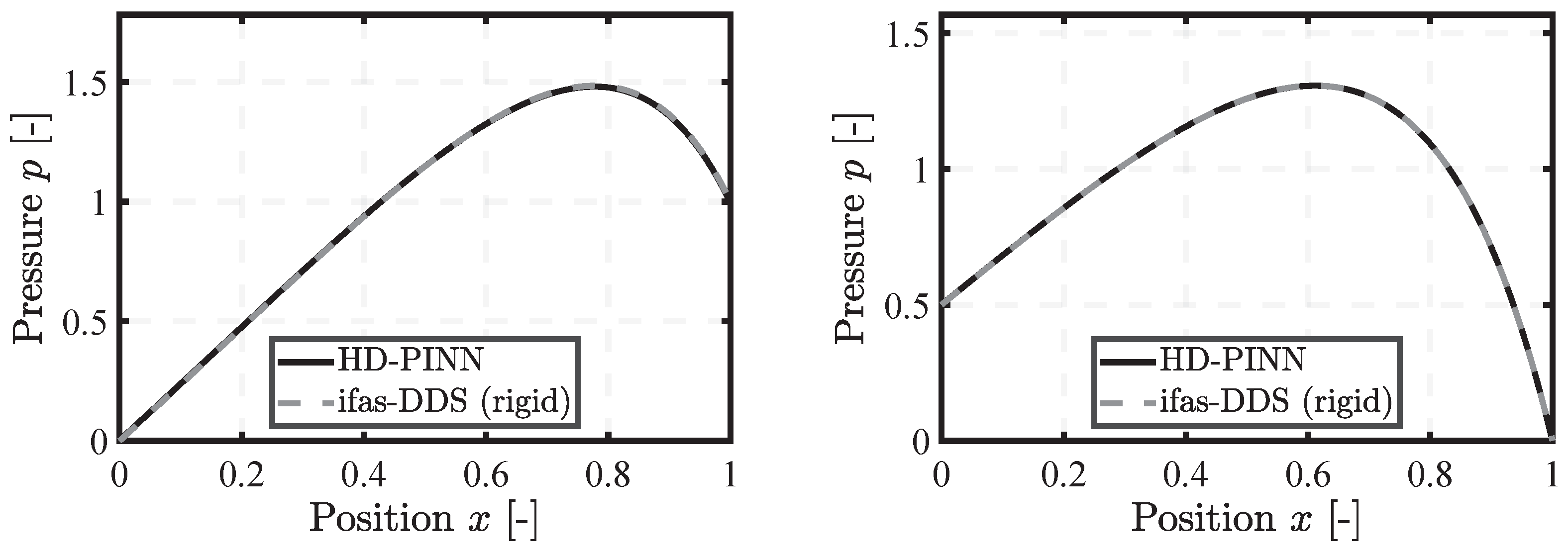
3.5. Position Extrapolation
4. Discussion
5. Conclusions
Author Contributions
Funding
Data Availability Statement
Conflicts of Interest
Abbreviations
| Adam | Adaptive moment estimation |
| EHL | Elastohydrodynamic lubrication |
| HD | Hydrodynamic |
| JFO | Jakobsson–Floberg–Olsson |
| MSE | Mean squared error |
| PDE | Partial differential equation |
| PINN | Physics-informed neural network |
| PIML | Physics-informed machine learning |
| ReLU | Rectified linear unit |
| ReLoBRaLo | Relative Loss Balancing with Random Lookback |
| SS | Swift–Stieber |
Nomenclature
| Symbol | Definition | Unit |
| h | Gap height | [-] |
| Height at left end | [-] | |
| Height at right end | [-] | |
| Curvature of sealing | [-] | |
| Position for sealing bend | [-] | |
| p | Hydrodynamic pressure | [-] |
| Pressure boundary condition for left and right boundary | [-] | |
| Pressure at the left and right boundary | [-] | |
| Root mean squared contact surface roughness | [-] | |
| t | Time | [-] |
| v | Velocity of counter surface | [-] |
| x | Axial coordinate | [-] |
| Position of sealing bend | [-] | |
| Left end of geometry | [-] | |
| Right end of geometry | [-] | |
| Fluid viscosity | [-] | |
| Cavity friction | [-] | |
| Fluid density | [-] | |
| Pressure flow factors | [-] | |
| Shear flow factors | [-] | |
| Partial derivative of pressure with regards to time and position | [-] |
References
- Bauer, N.; Sumbat, B.; Feldmeth, S.; Bauer, F.; Schmitz, K. Experimental determination and EHL simulation of transient friction of pneumatic seals in spool valves. In Proceedings of the Sealing Technology—Old School and Cutting Edge: International Sealing Conference: 21st ISC, Stuttgart, Germany, 7–8 October 2022; pp. 503–522. [Google Scholar]
- Cuomo, S.; Di Cola, V.S.; Giampaolo, F.; Rozza, G.; Raissi, M.; Piccialli, F. Scientific Machine Learning Through Physics–Informed Neural Networks: Where we are and What is Next. J. Sci. Comput. 2022, 92, 88. [Google Scholar] [CrossRef]
- Almqvist, A. Fundamentals of Physics-Informed Neural Networks Applied to Solve the Reynolds Boundary Value Problem. Lubricants 2021, 9, 82. [Google Scholar] [CrossRef]
- Zhao, Y.; Guo, L.; Wong, P.P.L. Application of physics-informed neural network in the analysis of hydrodynamic lubrication. Friction 2023, 11, 1253–1264. [Google Scholar] [CrossRef]
- Li, L.; Li, Y.; Du, Q.; Liu, T.; Xie, Y. ReF-nets: Physics-informed neural network for Reynolds equation of gas bearing. Comput. Methods Appl. Mech. Eng. 2022, 391, 114524. [Google Scholar] [CrossRef]
- Yadav, S.K.; Thakre, G. Solution of Lubrication Problems with Deep Neural Network. In Advances in Manufacturing Engineering; Dikshit, M.K., Soni, A., Davim, J.P., Eds.; Lecture Notes in Mechanical Engineering; Springer: Singapore, 2023; pp. 471–477. [Google Scholar] [CrossRef]
- Rom, M. Physics-informed neural networks for the Reynolds equation with cavitation modeling. Tribol. Int. 2023, 179, 108141. [Google Scholar] [CrossRef]
- Cheng, Y.; He, Q.; Huang, W.; Liu, Y.; Li, Y.; Li, D. HL-nets: Physics-informed neural networks for hydrodynamic lubrication with cavitation. Tribol. Int. 2023, 188, 108871. [Google Scholar] [CrossRef]
- Xi, Y.; Deng, J.; Li, Y. A new method to solve the Reynolds equation including mass-conserving cavitation by physics informed neural networks (PINNs) with both soft and hard constraints. Friction 2024, 12, 1165–1175. [Google Scholar] [CrossRef]
- Brumand-Poor, F.; Bauer, N.; Plückhahn, N.; Schmitz, K. Fast Computation of Lubricated Contacts: A Physics-Informed Deep Learning Approach. In Proceedings of the 14th International Fluid Power Conference: Fluid Power—Sustainable Productivity, Dresden, Germany, 19–21 March 2024. [Google Scholar]
- Bauer, N.; Baumann, M.; Feldmeth, S.; Bauer, F.; Schmitz, K. Elastohydrodynamic Simulation of Pneumatic Sealing Friction Considering 3D Surface Topography. Chem. Eng. Technol. 2023, 46, 167–174. [Google Scholar] [CrossRef]
- Bauer, N.; Rambaks, A.; Müller, C.; Murrenhoff, H.; Schmitz, K. Strategies for Implementing the Jakobsson-Floberg-Olsson Cavitation Model in EHL Simulations of Translational Seals. Int. J. Fluid Power 2021, 22, 199–232. [Google Scholar] [CrossRef]
- Angerhausen, J.; Woyciniuk, M.; Murrenhoff, H.; Schmitz, K. Simulation and experimental validation of translational hydraulic seal wear. Tribol. Int. 2019, 134, 296–307. [Google Scholar] [CrossRef]
- Marian, M.; Tremmel, S. Current Trends and Applications of Machine Learning in Tribology—A Review. Lubricants 2021, 9, 86. [Google Scholar] [CrossRef]
- Paturi, U.M.R.; Palakurthy, S.T.; Reddy, N.S. The Role of Machine Learning in Tribology: A Systematic Review. Arch. Comput. Methods Eng. 2023, 30, 1345–1397. [Google Scholar] [CrossRef]
- Kanai, R.A.; Desavale, R.G.; Chavan, S.P. Experimental-Based Fault Diagnosis of Rolling Bearings Using Artificial Neural Network. J. Tribol. 2016, 138, 4032525. [Google Scholar] [CrossRef]
- Sadık Ünlü, B.; Durmuş, H.; Meriç, C. Determination of tribological properties at CuSn10 alloy journal bearings by experimental and means of artificial neural networks method. Ind. Lubr. Tribol. 2012, 64, 258–264. [Google Scholar] [CrossRef]
- Canbulut, F.; Yildirim, Ş.; Sinanoğlu, C. Design of an Artificial Neural Network for Analysis of Frictional Power Loss of Hydrostatic Slipper Bearings. Tribol. Lett. 2004, 17, 887–899. [Google Scholar] [CrossRef]
- Hess, N.; Shang, L. Development of a Machine Learning Model for Elastohydrodynamic Pressure Prediction in Journal Bearings. J. Tribol. 2022, 144, 4053815. [Google Scholar] [CrossRef]
- Velioglu, M.; Mitsos, A.; Dahmen, M. Physics-Informed Neural Networks (PINNs) for Modeling Dynamic Processes Based on Limited Physical Knowledge and Data. In Proceedings of the 2023 AIChE Annual Meeting, Orlando, FL, USA, 5–10 November 2023. [Google Scholar]
- Psichogios, D.C.; Ungar, L.H. A hybrid neural network–first principles approach to process modeling. AIChE J. 1992, 38, 1499–1511. [Google Scholar] [CrossRef]
- Su, H.T.; Bhat, N.; Minderman, P.A.; McAvoy, T.J. Integrating Neural Networks with First Principles Models for Dynamic Modeling. IFAC Proc. Vol. 1992, 25, 327–332. [Google Scholar] [CrossRef]
- Kahrs, O.; Marquardt, W. The validity domain of hybrid models and its application in process optimization. Chem. Eng. Process. Process Intensif. 2007, 46, 1054–1066. [Google Scholar] [CrossRef]
- Marian, M.; Tremmel, S. Physics-Informed Machine Learning—An Emerging Trend in Tribology. Lubricants 2023, 11, 463. [Google Scholar] [CrossRef]
- Nabian, M.A.; Meidani, H. Physics-Driven Regularization of Deep Neural Networks for Enhanced Engineering Design and Analysis. J. Comput. Inf. Sci. Eng. 2020, 20, 436. [Google Scholar] [CrossRef]
- Lee, H.; Kang, I.S. Neural algorithm for solving differential equations. J. Comput. Phys. 1990, 91, 110–131. [Google Scholar] [CrossRef]
- Lagaris, I.E.; Likas, A.; Fotiadis, D.I. Artificial Neural Networks for Solving Ordinary and Partial Differential Equations. IEEE Trans. Neural Netw. 1998, 9, 987–1000. [Google Scholar] [CrossRef] [PubMed]
- Cybenko, G. Approximation by superpositions of a sigmoidal function. Math. Control. Signals Syst. 1989, 2, 303–314. [Google Scholar] [CrossRef]
- Hornik, K.; Stinchcombe, M.; White, H. Multilayer feedforward networks are universal approximators. Neural Netw. 1989, 2, 359–366. [Google Scholar] [CrossRef]
- Owhadi, H. Bayesian Numerical Homogenization. Multiscale Model. Simul. 2015, 13, 812–828. [Google Scholar] [CrossRef]
- Raissi, M.; Perdikaris, P.; Karniadakis, G.E. Inferring solutions of differential equations using noisy multi-fidelity data. J. Comput. Phys. 2017, 335, 736–746. [Google Scholar] [CrossRef]
- Raissi, M.; Perdikaris, P.; Karniadakis, G.E. Machine learning of linear differential equations using Gaussian processes. J. Comput. Phys. 2017, 348, 683–693. [Google Scholar] [CrossRef]
- Raissi, M.; Perdikaris, P.; Karniadakis, G.E. Numerical Gaussian Processes for Time-dependent and Non-linear Partial Differential Equations. Siam J. Sci. Comput. 2018, 40, 17M1120762. [Google Scholar] [CrossRef]
- Raissi, M.; Karniadakis, G.E. Hidden physics models: Machine learning of nonlinear partial differential equations. J. Comput. Phys. 2018, 357, 125–141. [Google Scholar] [CrossRef]
- Raissi, M.; Perdikaris, P.; Karniadakis, G.E. Physics Informed Deep Learning (Part I): Data-driven Solutions of Nonlinear Partial Differential Equations. J. Comput. Phys. 2019, 378, 686–707. [Google Scholar] [CrossRef]
- Raissi, M.; Perdikaris, P.; Karniadakis, G.E. Physics Informed Deep Learning (Part II): Data-driven Discovery of Nonlinear Partial Differential Equations. arXiv 2017, arXiv:1711.10566v1. [Google Scholar]
- Raissi, M.; Perdikaris, P.; Karniadakis, G.E. Physics-informed neural networks: A deep learning framework for solving forward and inverse problems involving nonlinear partial differential equations. J. Comput. Phys. 2019, 378, 686–707. [Google Scholar] [CrossRef]
- Antonelo, E.A.; Camponogara, E.; Seman, L.O.; Souza, E.R.d.; Jordanou, J.P.; Hubner, J.F. Physics-Informed Neural Nets for Control of Dynamical Systems. Neurocomputing 2024, 579, 127419. [Google Scholar] [CrossRef]
- Kim, J.; Lee, K.; Lee, D.; Jin, S.Y.; Park, N. DPM: A Novel Training Method for Physics-Informed Neural Networks in Extrapolation. arXiv 2021, arXiv:2012.02681v1. [Google Scholar] [CrossRef]
- Fesser, L.; D’Amico-Wong, L.; Qiu, R. Understanding and Mitigating Extrapolation Failures in Physics-Informed Neural Networks. arXiv 2023, arXiv:2306.09478v2. [Google Scholar]
- Baydin, A.G.; Pearlmutter, B.A.; Radul, A.A.; Siskind, J.M. Automatic differentiation in machine learning: A survey. Atilim Gunes Baydin. 2017, 18, 5595–5637. [Google Scholar]
- Cai, S.; Mao, Z.; Wang, Z.; Yin, M.; Karniadakis, G.E. Physics-informed neural networks (PINNs) for fluid mechanics: A review. Acta Mech. Sin. 2021, 37, 1727–1738. [Google Scholar] [CrossRef]
- Bischof, R.; Kraus, M. Multi-Objective Loss Balancing for Physics-Informed Deep Learning. arXiv 2021, arXiv:2110.09813v2. [Google Scholar] [CrossRef]
- Rimon, M.T.I.; Hassan, M.F.; Lyathakula, K.R.; Cesmeci, S.; Xu, H.; Tang, J. A Design Study of an Elasto-Hydrodynamic Seal for sCO2 Power Cycle by Using Physics Informed Neural Network. In Proceedings of the ASME Power Applied R&D 2023, American Society of Mechanical Engineers, Long Beach, CA, USA, 6–8 August 2023. [Google Scholar] [CrossRef]
- Kingma, D.P.; Ba, J. Adam: A Method for Stochastic Optimization. arXiv 2014, arXiv:1412.6980. [Google Scholar]
- Schmidt, R.M.; Schneider, F.; Hennig, P. Descending through a Crowded Valley—Benchmarking Deep Learning Optimizers. arXiv 2020, arXiv:2007.01547v6. [Google Scholar]
- Reyad, M.; Sarhan, A.M.; Arafa, M. A modified Adam algorithm for deep neural network optimization. Neural Comput. Appl. 2023, 35, 17095–17112. [Google Scholar] [CrossRef]
- Heydari, A.A.; Thompson, C.A.; Mehmood, A. SoftAdapt: Techniques for Adaptive Loss Weighting of Neural Networks with Multi-Part Loss Functions. arXiv 2019, arXiv:1912.12355. [Google Scholar]
- Wang, S.; Teng, Y.; Perdikaris, P. Understanding and mitigating gradient pathologies in physics-informed neural networks. arXiv 2020, arXiv:2001.04536. [Google Scholar] [CrossRef]
- Močkus, J. On bayesian methods for seeking the extremum. In Proceedings of the Optimization Techniques IFIP Technical Conference Novosibirsk, Novosibirsk, Russia, 1–7 July 1974; Goos, G., Hartmanis, J., Brinch Hansen, P., Gries, D., Moler, C., Seegmüller, G., Wirth, N., Marchuk, G.I., Eds.; Springer: Berlin/Heidelberg, Germany, 1975; Volume 27, pp. 400–404. [Google Scholar] [CrossRef]
- Escapil-Inchauspé, P.; Ruz, G.A. Hyper-parameter tuning of physics-informed neural networks: Application to Helmholtz problems. Neurocomputing 2023, 561, 126826. [Google Scholar] [CrossRef]


Disclaimer/Publisher’s Note: The statements, opinions and data contained in all publications are solely those of the individual author(s) and contributor(s) and not of MDPI and/or the editor(s). MDPI and/or the editor(s) disclaim responsibility for any injury to people or property resulting from any ideas, methods, instructions or products referred to in the content. |
© 2024 by the authors. Licensee MDPI, Basel, Switzerland. This article is an open access article distributed under the terms and conditions of the Creative Commons Attribution (CC BY) license (https://creativecommons.org/licenses/by/4.0/).
Share and Cite
Brumand-Poor, F.; Bauer, N.; Plückhahn, N.; Thebelt, M.; Woyda, S.; Schmitz, K. Extrapolation of Hydrodynamic Pressure in Lubricated Contacts: A Novel Multi-Case Physics-Informed Neural Network Framework. Lubricants 2024, 12, 122. https://doi.org/10.3390/lubricants12040122
Brumand-Poor F, Bauer N, Plückhahn N, Thebelt M, Woyda S, Schmitz K. Extrapolation of Hydrodynamic Pressure in Lubricated Contacts: A Novel Multi-Case Physics-Informed Neural Network Framework. Lubricants. 2024; 12(4):122. https://doi.org/10.3390/lubricants12040122
Chicago/Turabian StyleBrumand-Poor, Faras, Niklas Bauer, Nils Plückhahn, Matteo Thebelt, Silas Woyda, and Katharina Schmitz. 2024. "Extrapolation of Hydrodynamic Pressure in Lubricated Contacts: A Novel Multi-Case Physics-Informed Neural Network Framework" Lubricants 12, no. 4: 122. https://doi.org/10.3390/lubricants12040122