Abstract
This study investigates the effect of oil viscosity on pollutant emissions and fuel consumption of an internal combustion engine (ICE) at high altitudes using a response surface methodology (RSM). A Chevrolet Corsa Evolution 1.5 SOHC gasoline engine was used in Cuenca, Ecuador (2560 m above sea level), testing three lubricating oils with kinematic viscosities of 9.66, 14.08, and 18.5 mm2/s, measured at a temperature of 100 °C under various engine speeds and loads. Key findings include the following: hydrocarbon (HC) emissions were minimized from 150.22 ppm at the maximum load to 7.25 ppm with low viscosity and load; carbon dioxide (CO2) emissions peaked at 15.2% vol with high viscosity and load; carbon monoxide (CO) ranged from 0.04% to 3.74% depending on viscosity and load; nitrogen oxides (NOx) were significantly influenced by viscosity, RPM, and load, indicating a need for model refinement; and fuel consumption was significantly affected by load and viscosity. RSM-based optimization identified optimal operational conditions with a viscosity of 13 mm2/s, 1473 rpm, and a load of 78%, resulting in 52.35 ppm of HC, 13.97% vol of CO2, 1.2% vol of CO, 0 ppm of NOx, and a fuel consumption of 6.66 L/h. These conditions demonstrate the ability to adjust operational variables to maximize fuel efficiency and minimize emissions. This study underscores the critical role of optimizing lubricant viscosity and operational conditions to mitigate environmental impact and enhance engine performance in high-altitude environments.
1. Introduction
The exponential growth of the vehicle fleet in recent decades has generated a significant increase in polluting emissions, becoming one of the leading environmental challenges at a global level []. Road vehicle growth in developed and developing countries is projected to increase by 45% by 2025, affecting traffic, traffic density, and emissions []. In 2023, the EU approved a series of Commission suggestions to align the EU’s climate, energy, transport, and taxation policies to reduce net greenhouse gas emissions by at least 55% by 2030 compared with the 1990 levels. This initiative aims to make the EU the first climate-neutral continent by 2050 []. Therefore, reducing environmental pollutant emissions from internal combustion engines (ICEs) requires the development of more efficient engines in terms of fuel consumption, emission generation, and power density []. Harmful components of engine exhaust gases include nitrous oxides (NOx), carbon dioxide (CO2), carbon monoxide (CO), hydrocarbons (HC), and particulate matter (PM) [], which have a direct impact on air quality and are a significant risk factor for human health, contributing to global warming and acid rains [].
ICEs are complex systems involving various components: lubrication, friction, charge cycles, supercharging, mixture formation, ignition, combustion systems, electronics and mechanics for engine management, transmission shift control, powertrain, sensors, actuators, cooling, exhaust emissions, operating fluids, filtration, etc., providing alternatives to optimize its performance []. One of these alternatives to reduce fuel consumption and, therefore, minimize the emission of polluting gases into the environment is based on lowering mechanical losses and increasing engine efficiency []. In this regard, strategies have been developed to reduce these losses in the ICEs [,,,,].
Hybrid surface modification techniques, such as coatings, textures, and nanoparticles, can improve the tribological performance of engine components []. Improving surface coatings through micro-reliefs on the inner surface of cylinder liners can reduce mechanical losses in internal combustion engines by an average of 10.8% and increase mechanical efficiency by 4.0% [,]. Hazar et al. propose coating engine components with MgO-ZrO2 and ZrO2, which provides a thermal barrier, increasing engine power and reducing fuel consumption while decreasing pollutant emissions [].
On the other hand, downsizing internal combustion engines can improve fuel utilization, reduce emissions, and increase efficiency by reducing the weight of moving parts such as pistons and crankshafts [,], which can reduce CO2 emissions by about 18% in warm engine conditions for mid-class vehicles []. Podrigalo et al. conclude that a rational reduction in effective engine capacity can lead to a 9.5% reduction in fuel consumption while maintaining the specified maximum speed and dynamic properties of cars []. Likewise, reducing the gap between compression rings and increasing the twist angle can help reduce leakage flows by 37% and contribute to minimizing global emissions [].
Similarly, the use of low-viscosity oils (LVO) is adopted to reduce mechanical losses in ICEs due to the ease of implementation costs versus the advantages of reducing pollutant emissions and fuel consumption [,,,]. These oils reduce frictional power loss and wear load on compression ring surfaces, leading to maximum fuel economy in internal combustion engines []. LVO can reduce fuel consumption by around 2% in light-duty diesel engines [], and 5% in urban transport buses [] depending on the test conditions, offering a cost-effective way to increase engine efficiency and reduce CO2 emissions. Hawley et al. determine up to 3.5% fuel economy improvement in engines using lower-viscosity lubricants, compared with current production lubricants []. In the same way, Ishizaki et al. conclude that ultra-low viscosity engine oils can reduce CO2 emissions by 0.6% in 1.5–1.8 L gasoline engines in the New European Driving Cycles (NEDC) mode and improve fuel efficiency in passenger vehicles, but their cost-effectiveness depends on both viscosity reduction and oil drain interval extension []. However, the use of low-viscosity oils in ICE results in magnified wear due to thinner oil films and requires additional wear protection additives for effective performance [,].
Another factor that significantly affects fuel consumption and pollutant emissions is altitude. These altitude changes have a direct impact on the performance, fuel consumption, and emissions of ICEs []. Diesel vehicles, in particular, have higher CO2, CO, and NOx emission factors than gasoline vehicles. These emissions increase with altitude because there is lower atmospheric pressure, temperature, and oxygen concentration, resulting in reduced combustion efficiency in automotive engines with atmospheric pressure being the primary environmental factor affecting emissions [] by lengthening the ignition delay, increasing energy release, and prolonging the late combustion period, leading to reduced thermal and combustion efficiency []. Wan et al. declare that as altitude increases from 0 to 2000 m, engine torque drops by 2.9%, brake-specific fuel consumption (BSFC) increases by 2.6%, NOx emissions reduce by 11.8%, and opacity smoke increases by 26.2% []. He et al. state that high altitude increases diesel engine emissions of HC, CO, and smoke, with average increases of 30%, 34%, and 35% at 1000 m []. NOx emissions vary with engine types and working conditions [].
2. Materials and Methods
2.1. Description of the Experimental Setup
For the present study, a data acquisition protocol is established through an experimental design using the response surface methodology (RSM), which will allow for visual analysis of the average result for a particular area of the levels of the input factors or variables such as lubricant viscosity, engine speed, and applied load, thus evaluating the sensitivity of the output variables (emissions and fuel consumption) to such changes in operating conditions.
In this study, the experiments were performed on a Chevrolet Corsa Evolution 1.5 SOHC, four-cylinder, four-stroke, and SI (spark ignition) gasoline engine in the city of Cuenca, Ecuador, which is located 2560 m above sea level. The engine specification is given in Table 1.

Table 1.
Main characteristics of the test engine.
This vehicle is mounted on a dynamometer MAHA LPS 3000, which is composed of eddy current dynamometer brakes, which, in addition to measuring traction and power at the same time, can also generate loads with revolutions within a range of 0–10,000 rpm, speed from 0 to 260 km/h and constant tractive force from 0 to 6 KN, as shown in Figure 1. The dynamometer is also equipped with an AIC 5008 fuel flow meter capable of measuring volumetric flow rate from 0 to 120 L/h with a sensitivity of 0.01.

Figure 1.
Experimental unit.
Exhaust gases were measured using a Brain Bee AGS-688 analyzer (Mahle, Stuttgart, Germany), which can determine the different concentrations of HC, CO, CO2, O2, and NOx emitted in the experimental unit vehicle, as shown in Table 2.
Table 2.
Technical specifications of the gas analyzer.
The levels of the input variable, oil viscosity, are characterized by the kinematic viscosity measured in mm2/s @ 100 °C of three lubricants, primarily composed of a synthetic base of polyalphaolefins (PAO), which constitute between 70% and 90% of the formulation. Synthetic esters, ranging from 10% to 20%, are also included to enhance lubricating properties. The formulation is completed with a variety of additives that represent between 10% and 20% of the formulated oil. These additives include detergents (1–3%), dispersants (3–5%), antioxidants (1–2%), corrosion inhibitors (0.5–1%), viscosity index improvers (2–5%), friction modifiers (0.1–1%), anti-wear additives (1–2%), and anti-foaming agents (<0.1%), whose technical specifications are shown in Table 3.
Table 3.
Technical specifications of the oils used in the study.
2.2. Response Surface Methodology
The response surface methodology (RSM) is based on several mathematical and statistical methodologies that are used to develop a suitable functional relationship between a factor of interest , and certain control (input) variables denoted by . These variables can include factors such as oil viscosity, engine speed, and applied load in our study where . This relationship is not commonly known but can be approximated by a polynomial model of lower degree as expressed in Equation (1):
where , represents a p-element vector function consisting of powers and cross products of powers of until reaching a certain degree denoted by . is a vector of p coefficients, which are constant and unknown being denoted as parameters, and is the random experimental error, assumed to have zero mean. This is conditional on the idea that the model in Equation (1) provides an adequate representation of the response. In this case, the quantity represents the mean response, i.e., the expected value of y, and is denoted by . Typically, the response surface methodology uses two important models. These are special cases of the model presented in Equation (1). Equation (2) presents the first-degree polynomial model :
where represents the -th input variable, and is the coefficient corresponding to the linear term of . In this case, the terms are simply the individual input variables.
Equation (3) states the second-degree model :
where is the number of input variables, for this study ; , and represent these individual input variables. is the constant term, is the coefficient of the linear term , is the coefficient of the quadratic term , and is the coefficient of the interaction of the terms . Finally, is the residual associated with the experiment. In this study, a Box–Behnken design is applied, which gives comparatively precise results. Table 4 shows the input variables and levels. Table 5 shows the design table that contains the data from 17 experiments.
Table 4.
Input variables and levels of the experiment.
Table 5.
Table of design related to the experimental results.
Figure 2 shows a schematic illustration of the experimental setup. The test vehicle is mounted on the dynamometer (a), which monitors the speed and load (b). Inference variables such as coolant temperature, wheels, and lubricant are monitored through the dynamometer’s sensor console (c). During data acquisition, fuel flow (d) and pollutant emissions (e) are recorded to finally analyze the data obtained in the experiment through specific software (f).
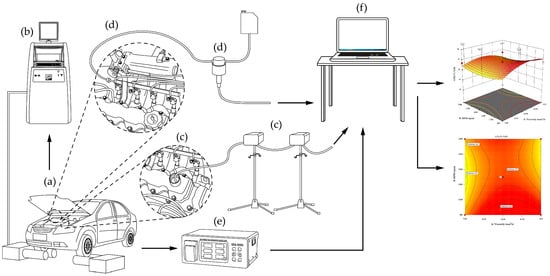
Figure 2.
Schematic of the experimental setup. (a) Dynamometer. (b) Dynamometer control unit. (c) Dynamometer’s sensor console. (d) Fuel flow meter. (e) Gas emissions analyzer. (f) Expert design software (version 12).
3. Results
3.1. Model for HC
The ANOVA results and fit statistics for HC are presented in Table 6. The ANOVA analysis of the quadratic model indicates that the model is significant, with an F-value of 6.36 and a p-value of 0.0117, suggesting a statistically significant impact of the studied factors on the HC response. Among the individual terms, load (C) emerges as the most influential factor, with an F-value of 27.61 and a p-value of 0.0012, highlighting its critical importance in the model. The quadratic term of load (C2) is also significant, with an F-value of 16.38 and a p-value of 0.0049, indicating a robust nonlinear relationship between the load and the response. In contrast, viscosity (A) and the interactions between factors (AB, AC) were not significant (p > 0.78). While the interaction BC and the quadratic term of RPM (B2) showed trends toward significance (p ≈ 0.06 and p ≈ 0.12, respectively), they did not meet the critical threshold. The model’s R2 value is 0.8910 (refer to Table 7), indicating that it explains 89.10% of the variability in the data, while the adjusted R2 is 0.7509, reflecting a decrease in explanatory power when accounting for the number of terms in the model. However, the predicted R2 is −0.7362, implying poor predictive performance and suggesting that the overall mean might be a better predictor than the current model. The significant lack of fit, with an F-value of 278.41 and an extremely low p-value (p < 0.0001), indicates that the model does not fully capture the observed variations, underscoring the need to explore more complex models or consider additional factors. The actual regression equation for HC is given in Equation (4).
HC [ppm] = 240.5 − 39.28 × Viscosity + 0.07 × RPM − 2.38 × Load + 0.0008 × Viscosity × RPM − 0.02 × Viscosity × Load + 0.0008 × RPM × Load + 1.37 × Viscosity2 − 2.93 × 10⁻⁵ × RPM2 + 0.025 × Load2
Table 6.
ANOVA results for HC.
Table 7.
Coefficient of determination for HC.
The contour plot (see Figure 3a) shows the interrelation of variables, with viscosity ranging from 9.66 to 18.5 mm2/s and load spanning from 0% to 100%. Notable predictions include an HC emission of 150.22 ppm at maximum load (100%) and viscosity (18.5 mm2/s), represented in reddish tones, suggesting a significant increase in emissions under these conditions. Conversely, at a minimal load of 5% and viscosity of 9.66 mm2/s, HC emissions decrease to 7.26 ppm, indicated in bluish tones, showing a marked reduction. The surface plot of Figure 3b corroborates these findings, illustrating a pronounced curvature indicative of a nonlinear relationship between the independent variables and HC emissions. The 3D plot reveals that a low viscosity of 9.66 mm2/s combined with a low load of 5% results in HC emissions of 7.26 ppm, while a viscosity of 18.5 mm2/s and a load of 100% produce 150.22 ppm of HC. This analysis underscores the critical need to optimize lubrication parameters to mitigate environmental impact, emphasizing the influence of lubricant viscosity and operational load on emissions.

Figure 3.
(a) Contour plot and (b) response surface for HC.
3.2. Model for CO2
Presented in Table 8 are the ANOVA results and fit statistics for CO2. The model is significant, as evidenced by the F-value of 4.59 and a p-value of 0.0285. Additionally, terms C and C2 (C-Load) are individually significant, suggesting their influence on the response variable. However, a considerable lack of fit is observed, as indicated by the high lack of fit F-value of 397.92 and an extremely low p-value. Regarding the fit statistics (refer to Table 9), the coefficient of determination R2 indicates that the model explains approximately 85.5% of the total variability in the data. At the same time, the adjusted R2, at 0.6687, reflects a corrected measure considering the number of terms in the model. Despite the model’s high capability to explain variability, the lack of fit underscores the need for improved predictive accuracy. The regression equation for CO2 is provided in Equation (5).
CO2 [% vol] = 8.9 + 0.82 × Viscosity − 0.0002 × RPM + 0.04 × Load − 0.00005 × Viscosity × RPM − 0.0001 × Viscosity × Load − 0.00002 × RPM × Load − 0.025 × Viscosity2 + 4.36 × 10⁻⁷ × RPM2 − 0.0003 × Load2
Table 8.
ANOVA results for CO2.
Table 9.
Coefficient of determination for CO2.
The contour plot of Figure 4a illustrates the response surface predictions with various levels ranging from 14.2 to 15.15% vol. The critical design points marked in red indicate significant regions where the response variable peaks or valleys are observed. For instance, the contour lines show that the response value is approximately 14.4 near the design points, increasing to around 15.15 at the lower edge of the plot. This gradient highlights a clear response trend as one moves through the design space, indicating regions of high and low responses.
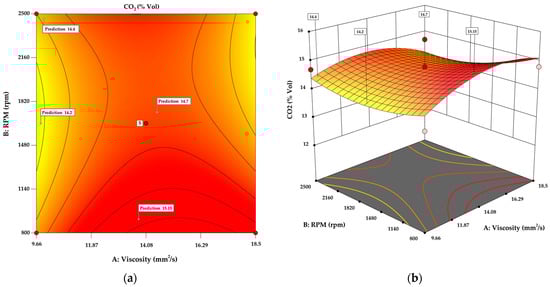
Figure 4.
(a) Contour plot and (b) response surface for CO2.
The surface plot of Figure 4b reveals the response surface’s three-dimensional aspects, visually representing how the response variable changes across the design space. The surface’s curvature suggests a nonlinear relationship between the independent variables and the response. Specific predictions at notable points, such as 14.4, 14.2, and 15.15, are highlighted, indicating areas where the response variable exhibits significant changes. The upper surface portion shows a prediction value of 14.7, demonstrating a peak in the response.
3.3. Model for CO
Table 10 outlines the ANOVA results and fit statistics for CO. The analysis of the evaluated quadratic model reveals significant results and provides a detailed view of the influence of various variables on the studied response. The primary factors evaluated include viscosity (A), RPM (B), and load (C). The model, as a whole, is significant (p = 0.0107), indicating that, in general, the variables included in the model have a relevant impact on the response. Among the individual factors, the variable load (C) shows considerable significance (p = 0.0009), suggesting that the load has a notable effect on the response. On the other hand, the variables of viscosity (A) and RPM (B) do not exhibit individual statistical significance (p = 0.9569 and p = 0.1232, respectively). Interactions between variables, such as AB and AC, also do not show significance, indicating that there are no relevant synergistic effects between these factors within the model. The coefficient of determination (R2) of 0.8941 suggests that the model explains 89.41% of the observed variability in the data, which is relatively high, as shown in Table 11. However, the adjusted R2 is significantly lower (0.7579), suggesting that some variables may not be contributing efficiently to explaining the variability. The model’s adequate precision is 8.2728, indicating a good signal-to-noise ratio, essential for the reliability of predictions. The regression equation for CO is detailed in Equation (6).
CO [% vol] = 4.74 − 0.83 × Viscosity + 0.002 × RPM − 0.074 × Load + 1.13 × 10⁻¹⁸ × Viscosity × RPM + 0.0002 × Viscosity × Load + 0.000024 × RPM × Load + 0.03 × Viscosity2 − 7.97 × 10⁻⁷ × RPM2 + 0.00064 × Load2
Table 10.
ANOVA results for CO.
Table 11.
Coefficient of determination for CO.
The contour graph for CO (see Figure 5a) displays a significant variation in CO concentration depending on the levels of viscosity and load, with values ranging from a minimum of 0.042 in areas of low viscosity and load to a maximum of 3.74 under conditions of high viscosity and increased load. In this graph, a color gradient transitions from blue (low CO concentration) to yellow (high CO concentration), highlighting the impact of the interactions between viscosity and load on CO production. For instance, the CO value is 0.072 at a point with intermediate viscosity and load, escalating dramatically to 3.11 and 3.74 in regions where both variables reach higher levels. This pattern suggests that an increase in viscosity, possibly in conjunction with higher load, elevates CO concentration, indicating a strong correlation between these variables.

Figure 5.
(a) Contour plot and (b) Response surface for CO.
The surface plot of Figure 5b provides a three-dimensional representation of these effects, showing how the response surface rises with increases in viscosity and load. The curvature of this surface clearly illustrates how specific adjustments in these input variables can lead to the maximization or minimization of CO production.
3.4. Model for NOx
Table 12 provides the ANOVA results and fit statistics for NOx. The analysis shows the model is significant, with a model F-value of 12.96. This high F-value corresponds to a probability of only 0.14% that such a result could occur due to random noise, affirming the model’s statistical significance. Significant model terms are identified by p-values less than 0.0500. In this case, the terms B, C, BC, A2, and B2 are significant, indicating their substantial impact on the NOx response. Conversely, terms with p-values greater than 0.1000 are considered insignificant and may warrant removal for model simplification. However, a notable concern is the discrepancy between the predicted R2 of 0.0941 and the adjusted R2 of 0.8706 (Table 13). This significant difference, exceeding 0.2, suggests potential issues with the model or data, such as a large block effect and the presence of outliers or other anomalies. Exploring model reduction, response transformation, and the identification of outliers is recommended to address this discrepancy. Moreover, conducting confirmation runs is essential to validating the empirical model. The adequate precision ratio of 10.719 exceeds the desirable threshold of 4, indicating a strong signal-to-noise ratio. This high ratio suggests that the model is reliable and can effectively navigate the design space for the NOx response. Despite the model’s overall significance and adequate signal strength, the substantial gap between the predicted and adjusted R2 values necessitates further refinement and validation to ensure the model’s robustness and accuracy. In conclusion, while the NOx response model shows strong potential with significant terms and an adequate signal, addressing the underlying issues indicated by the R2 discrepancy is crucial for enhancing model reliability and predictive performance. The regression equation for NOx is provided in Equation (7).
NOx [ppm] = 1264.76 − 124.4 × Viscosity − 0.63 × RPM − 5.3 × Load − 0.004 × Viscosity × RPM + 0.26 × Viscosity × Load + 0.002 × RPM × Load + 4.5 × Viscosity2 + 0.0002 × RPM2 − 0.0012 × Load2
Table 12.
ANOVA results for NOx.
Table 13.
Coefficient of determination for NOx.
In the contour graph of Figure 6a, NOx concentration exhibits a broad range, with a notable minimum of 0.25 located near the center of the lower edge, indicative of moderate load and high viscosity conditions. An intermediate value of 118.62 at the graph’s center reflects a moderate NOx response under median viscosity and load conditions. The observed maximum of 250.69 in the top right corner reveals that a combination of high viscosity and high load leads to the highest production of NOx, highlighting a strong interaction between these two variables. The surface plot offers a three-dimensional perspective, demonstrating how NOx levels escalate in response to increments in both variables. The surface of Figure 6b illustrates a gradual increase in NOx from the center toward the top right corner, indicating that the highest concentrations are achieved under extreme conditions of both variables.

Figure 6.
(a) Contour plot and (b) Response surface for NOx.
3.5. Model for Consumption
Table 14 displays the ANOVA results and fit statistics for consumption. The model is significant, with an F-value of 11.05. This high F-value suggests that there is only a 0.01% chance that such a result could occur due to random noise, confirming the model’s statistical significance. Significant model terms are identified by p-values less than 0.0500; in this case, the terms C, A2, B2, and C2 are significant, demonstrating their considerable impact on the consumption response. Conversely, terms with p-values more significant than 0.1000 are considered insignificant and may be candidates for model reduction to improve efficiency. However, the lack of fit F-value of 5.60 indicates a significant lack of fit. This is problematic, as we desire the model to fit well to the data, and there is only a 0.34% chance that this high lack of fit F-value is due to noise. A significant lack of fit suggests that the model does not adequately capture the observed variability in the data. Regarding the fit statistics, the standard deviation is 0.8548, and the R2 is 0.7397, indicating that the model explains 73.97% of the variability in the data. However, the adjusted R2 is 0.6728, and the predicted R2 is negative (−0.6143), suggesting that the overall mean might better predict the response than the current model (see Table 15). In such cases, a higher-order model may also predict better. The adequate precision, with a signal-to-noise ratio of 16.958, exceeds the desirable threshold of 4, indicating a strong signal and confirming that the model can navigate the design space effectively. The regression equation for consumption is detailed in Equation (8).
Consumption [L/h] = 14.5 − 2.14 × Viscosity + 0.0075 × RPM − 0.036 × Load − 0.00012 × Viscosity × RPM + 0.0012 × Viscosity × Load − 1.63 × 10⁻⁵ × RPM × Load + 0.08 × Viscosity2 − 1.61 × 10⁻⁶ × RPM2 + 0.0008 × Load2
Table 14.
ANOVA results for consumption.
Table 15.
Coefficient of determination for consumption.
The contour and surface plots presented in Figure 7 provide an in-depth analysis of how input variables, viscosity (x-axis) and load (y-axis), influence fuel consumption in a controlled experimental setting. These graphs depict significant variations in fuel consumption based on these variables. In the contour graph (Figure 7a), fuel consumption values range from 5.53 to 10.38, illustrating a distinct trend where consumption increases with load and viscosity. The lower consumption values, such as 5.53 and 5.37, are found in the central region, suggesting moderate conditions of load and viscosity. Conversely, the highest consumption values, reaching up to 10.38, are located in the upper right corner of the graph, indicating high load and viscosity conditions.
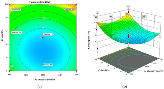
Figure 7.
(a) Contour plot and (b) response surface of consumption.
The surface plot of Figure 7b presents a three-dimensional representation of these effects, showing how fuel consumption escalates with increases in viscosity and load. The surface’s curvature clearly demonstrates a direct relationship between increased load and viscosity and higher fuel consumption.
This analysis is essential for developing effective fuel management strategies. It enables the identification of operational configurations that minimize consumption and enhance energy efficiency in internal combustion engines. Understanding the interplay between viscosity and load in relation to fuel consumption provides valuable opportunities for resource optimization and operational sustainability.
4. RSM-Based Optimization
An RSM-based optimization is a method to explore the shape and location of the maximum or minimum of a surface that mathematically represents the relationship between one or more responses and the influencing factors. In the current work, the emissions and fuel consumption of the engine are optimized. In this setup, shown in Table 16, the goal of minimum criteria was selected. Moreover, the default in the range criterion for study factors was selected.
Table 16.
Optimization setup.
The engine operating conditions identified by optimization were 13 mm2/s for viscosity, 1472 rpm, and 78% engine load (red dots), rounded to the nearest whole number. The response variables, corresponding to optimized operating conditions (blue dots), were 52.4 ppm of HC, 14% vol of CO2, 1.2% vol of CO, 0 ppm for NOx, and 6.7 L/h for consumption. The optimum gained values of study factors and response variables are shown by the red and blue dots in Figure 8.
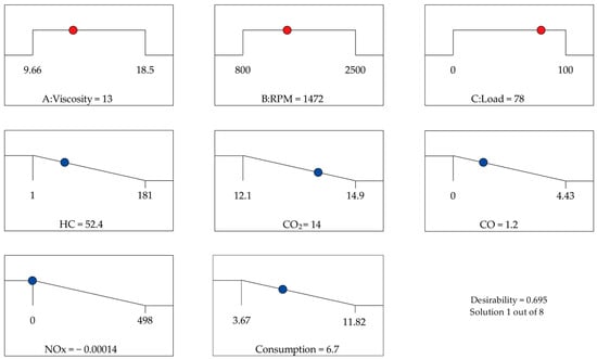
Figure 8.
Identified optimum point.
The statistical analysis of optimization and its impact on overall responses was examined using composite desirability (D). This metric, which ranges from 0 to 1, assigns a value of 1 to the best outcomes and 0 to the worst. In this study, the composite desirability achieved a value of 0.695, indicating that the optimization settings yielded positive results for all responses. Figure 9 displays the contour plot of desirability.

Figure 9.
Contour plot of desirability.
5. Discussion
The findings of this study underscore the significant influence of oil viscosity on pollutant emissions and fuel consumption in internal combustion engines at high altitudes, as evidenced by ANOVA analyses. Reducing HC emissions to 7.25 ppm with low-viscosity oils and reduced load highlights that appropriate lubricant selection could be an effective strategy to meet stricter environmental regulations without compromising engine performance. These results are consistent with previous studies, which demonstrated that lower-viscosity lubricants can reduce internal engine friction, thus decreasing pollutant emissions.
The evaluation of the HC model revealed a significant lack of fit (F-value of 278.41, p < 0.0001), suggesting that the current model does not fully capture the variability in the data. This lack of fit may be due to several factors, including the simplicity of the model, the absence of higher-order interactions or important nonlinear effects, and significant variability in the experimental data not explained by the model. To improve the model fit, it is suggested to include higher-order polynomial terms and additional interaction terms that can capture more complex relationships. Furthermore, it would be beneficial to explore data transformation techniques, such as logarithmic or Box-Cox transformation, to stabilize the variance and improve the model fit. Considering alternative modeling approaches, such as generalized additive models (GAMs) or machine learning techniques (e.g., random forest, gradient boosting), is also recommended, as they could more effectively capture nonlinear relationships and interactions present in the data. Additionally, it is suggested to review and, possibly, improve the current experimental design. Using more complex designs, such as the central composite design (CCD) or Box–Behnken design, could improve the estimation of quadratic effects and interactions. These improvements in experimental design and analysis methods would provide a more accurate and robust representation of the factors influencing HC emissions.
The negative predicted R2 values for HC (−0.7362) and CO2 (−1.3124) indicate poor predictive performance of the current model. This suggests that the model not only fails to adequately capture the underlying relationships between variables but may also be overfitted to the training data. Reasons for this lack of fit may include inadequate model structure, absence of interaction and higher-order terms, insufficient or unrepresentative data, and variability in the data due to measurement errors or unaccounted external factors. To improve predictive performance, it is proposed to simplify the model by removing nonsignificant terms, including higher-order polynomial and interaction terms, apply data transformation techniques, increase the quantity and quality of the data, use cross-validation techniques, and explore alternative modeling approaches, such as generalized additive models (GAMs) and machine learning methods.
Moreover, the peak in CO2 emissions observed with high-viscosity oils under heavy loads underscores the direct relationship between engine operating conditions and the production of greenhouse gases. This outcome, reinforced by significant ANOVA results, supports the hypothesis that interventions in lubricant formulation and engine operating conditions can play a critical role in mitigating climate change, aligning with global initiatives for carbon reduction.
RSM-based optimization reveals that adjusting the oil viscosity to 13 mm2/s, along with specific speed and load settings, optimally reduces emissions while maintaining fuel efficiency. This approach provides a robust framework for future research and encourages the exploration of different types of oils and engine design modifications that could further improve performance and environmental sustainability.
Future research could benefit from expanding the range of tested environmental and operational conditions, including different types of fuels and engine configurations, as suggested by the ANOVA models’ interaction terms. Additionally, incorporating life cycle analysis to assess the environmental impacts of lubricant production and disposal could provide a more comprehensive understanding of the total ecological footprint.
Further investigation into developing new lubricant compounds that operate effectively across a broader range of temperatures and pressures, mainly designed for high-altitude conditions, would be valuable. Exploring the interaction between these lubricants and hybrid or electric engine technologies could also lead to integrated strategies that maximize energy efficiency and minimize emissions across the entire vehicular system.
Author Contributions
Conceptualization, M.G.T., O.C.O. and F.C.M.; methodology, M.G.T.; investigation, O.C.O. and F.C.M.; writing—original draft preparation, M.G.T., O.C.O. and F.C.M.; writing—review and editing, M.G.T.; supervision, M.G.T. All authors have read and agreed to the published version of the manuscript.
Funding
This research received no external funding.
Data Availability Statement
The data presented in this study are available in Table 5.
Conflicts of Interest
The authors declare no conflicts of interest.
References
- Pischinger, S. Current and Future Challenges for Automotive Catalysis: Engine Technology Trends and Their Impact. Top. Catal. 2016, 59, 834–844. [Google Scholar] [CrossRef]
- Dargay, J. Road Vehicles: Future Growth in Developed and Developing Countries. Proc. Inst. Civ. Eng.-Munic. Eng. 2002, 151, 3–11. [Google Scholar] [CrossRef]
- 2030 Climate Targets-European Commission. Available online: https://climate.ec.europa.eu/eu-action/climate-strategies-targets/2030-climate-targets_en (accessed on 15 May 2024).
- Beles, H.; Tusinean, A.; Mitran, T.; Scurt, F.B. Research Regarding the Development of the Combustion Chamber of Internal Combustion Engines with Opposite Pistons. Machines 2023, 11, 309. [Google Scholar] [CrossRef]
- Khoa, N.X.; Lim, O. A Review of the External and Internal Residual Exhaust Gas in the Internal Combustion Engine. Energies 2022, 15, 1208. [Google Scholar] [CrossRef]
- Morgunov, B.; Chashchin, V.; Gudkov, A.; Chashchin, M.; Popova, O.; Nikanov, A.; Thomassen, Y. Health Risk Factors of Emissions from Internal Combustion Engine Vehicles: An Up-to-Date Status of the Problem. Здoрoвье Населения И Среда Обитания-ЗНиСО/Public Health Life Environ. 2022, 30, 7–14. [Google Scholar] [CrossRef]
- Van Basshuysen, R.; Schaefer, F. Internal Combustion Engine Handbook Basics, Components, Systems, and Perspectives; SAE International: Warrendale, PA, USA, 2004; ISBN 978-0-7680-1139-5. [Google Scholar]
- Payri González, F.; Desantes Fernández, J.M. Motores de Combustión Interna Alternativos; Editorial Universitat Politécnica de Valencia: Valencia, Spain, 2011; ISBN 8483637057. [Google Scholar]
- Posmyk, A. Influence of Material Properties on the Wear of Composite Coatings. Wear 2003, 254, 399–407. [Google Scholar] [CrossRef]
- Etsion, I.; Sher, E. Improving Fuel Efficiency with Laser Surface Textured Piston Rings. Tribol. Int. 2009, 42, 542–547. [Google Scholar] [CrossRef]
- Silva, C.; Ross, M.; Farias, T. Analysis and Simulation of “Low-Cost” Strategies to Reduce Fuel Consumption and Emissions in Conventional Gasoline Light-Duty Vehicles. Energy Convers. Manag. 2009, 50, 215–222. [Google Scholar] [CrossRef]
- Fontaras, G.; Vouitsis, E.; Samaras, Z. Experimental Evaluation of the Fuel Consumption and Emissions Reduction Potential of Low Viscosity Lubricants; SAE Technical Paper; SAE International: Warrendale, PA, USA, 2009. [Google Scholar]
- Macián, V.; Tormos, B.; Bermúdez, V.; Ramírez, L. Assessment of the Effect of Low Viscosity Oils Usage on a Light Duty Diesel Engine Fuel Consumption in Stationary and Transient Conditions. Tribol. Int. 2014, 79, 132–139. [Google Scholar] [CrossRef]
- Murari, G.; Nahak, B.; Pratap, T. Hybrid Surface Modification for Improved Tribological Performance of IC Engine Components—A Review. Proc. Inst. Mech. Eng. Part E J. Process Mech. Eng. 2023, 095440892211507. [Google Scholar] [CrossRef]
- Ha Hiep, N.; Cong Doan, N.; Quoc Quan, N.; Van Duong, N. Structural Modifications of the Inner Surface of Cylinder Liners for Decreasing Mechanical Losses in High-Speed Diesel Engines; SAE Technical Paper; SAE International: Warrendale, PA, USA, 2023. [Google Scholar]
- Hazar, H. Effects of Biodiesel on a Low Heat Loss Diesel Engine. Renew. Energy 2009, 34, 1533–1537. [Google Scholar] [CrossRef]
- Balaji, M.; Sarfas, M.; Vishaal, G.S.B.; Madhusudhan, G.V.; Gupta, S.; Kanchan, S. Scope for Improving the Efficiency and Environmental Impact of Internal Combustion Engines Using Engine Downsizing Approach: A Comprehensive Case Study. IOP Conf. Ser. Mater. Sci. Eng. 2021, 1116, 012070. [Google Scholar] [CrossRef]
- Menon, S.; Cadou, C. Scaling of Losses in Small IC Aero Engines with Engine Size. In Proceedings of the 42nd AIAA Aerospace Sciences Meeting and Exhibit, American Institute of Aeronautics and Astronautics, Reston, VA, USA, 5–8 January 2004. [Google Scholar]
- Leduc, P.; Dubar, B.; Ranini, A.; Monnier, G. Downsizing of Gasoline Engine: An Efficient Way to Reduce CO2 Emissions. Oil Gas Sci. Technol. 2003, 58, 115–127. [Google Scholar] [CrossRef]
- Podrigalo, M.; Tarasov, Y.; Kholodov, M.; Shein, V.; Tkachenko, A.; Kasianenko, O. Assessment of Increased Energy Efficiency of Vehicles with a Rational Reduction of Engine Capacity. Automob. Transp. 2022, 26–34. [Google Scholar] [CrossRef]
- Hernández-Comas, B.; Maestre-Cambronel, D.; Pardo-García, C.; Fonseca-Vigoya, M.D.S.; Pabón-León, J. Influence of Compression Rings on the Dynamic Characteristics and Sealing Capacity of the Combustion Chamber in Diesel Engines. Lubricants 2021, 9, 25. [Google Scholar] [CrossRef]
- Fan, Q.; Wang, Y.; Xiao, J.; Wang, Z.; Li, W.; Jia, T.; Zheng, B.; Taylor, R. Effect of Oil Viscosity and Driving Mode on Oil Dilution and Transient Emissions Including Particle Number in Plug-In Hybrid Electric Vehicle; SAE Technical Paper; SAE International: Warrendale, PA, USA, 2020. [Google Scholar]
- Taylor, R.I.; Coy, R.C. Improved Fuel Efficiency by Lubricant Design: A Review. Proc. Inst. Mech. Eng. Part J J. Eng. Tribol. 2000, 214, 1–15. [Google Scholar] [CrossRef]
- Hei, D.; Zheng, M.; Liu, C.; Jiang, L.; Zhang, Y.; Zhao, X. Study on the Frictional Properties of the Top Ring-Liner Conjunction for Different-Viscosity Lubricant. Adv. Mech. Eng. 2023, 15, 168781322311550. [Google Scholar] [CrossRef]
- Macián, V.; Tormos, B.; Ramírez, L.; Pérez, T.; Martínez, J. CO2 Emissions Reduction by Using Low Viscosity Oils in Public Urban Bus Fleets. WIT Trans. Built Environ. 2015, 14, 255–266. [Google Scholar]
- Hawley, J.G.; Bannister, C.D.; Brace, C.J.; Akehurst, S.; Pegg, I.; Avery, M.R. The Effect of Engine and Transmission Oil Viscometrics on Vehicle Fuel Consumption. Proc. Inst. Mech. Eng. Part D J. Automob. Eng. 2010, 224, 1213–1228. [Google Scholar] [CrossRef]
- Ishizaki, K.; Nakano, M. Reduction of CO2 Emissions and Cost Analysis of Ultra-Low Viscosity Engine Oil. Lubricants 2018, 6, 102. [Google Scholar] [CrossRef]
- Minami, I.; Murakami, H.; Nanao, H.; Mori, S. Additive Effect for Environmental Lubricants—Decreased Phosphorus Contents in Low Viscosity Base Oils for Antiwear Performance. J. Jpn. Pet. Inst. 2006, 49, 268–273. [Google Scholar] [CrossRef]
- Taylor, C.M. Engine Tribology; Elsevier: Amsterdam, The Netherlands, 1993; Volume 26, ISBN 0080875904. [Google Scholar]
- Ceballos, J.J.; Melgar, A.; Tinaut, F.V. Influence of Environmental Changes Due to Altitude on Performance, Fuel Consumption and Emissions of a Naturally Aspirated Diesel Engine. Energies 2021, 14, 5346. [Google Scholar] [CrossRef]
- Qi, Z.; Gu, M.; Cao, J.; Zhang, Z.; You, C.; Zhan, Y.; Ma, Z.; Huang, W. The Effects of Varying Altitudes on the Rates of Emissions from Diesel and Gasoline Vehicles Using a Portable Emission Measurement System. Atmosphere 2023, 14, 1739. [Google Scholar] [CrossRef]
- Liu, Z.; Liu, J. Investigation of the Effect of Simulated Atmospheric Conditions at Different Altitudes on the Combustion Process in a Heavy-Duty Diesel Engine Based on Zero-Dimensional Modeling. J. Eng. Gas Turbines Power 2022, 144, 061013. [Google Scholar] [CrossRef]
- Wan, M.; Huang, F.; Shen, L.; Lei, J. Experimental Investigation on Effects of Fuel Injection and Intake Parameters on Combustion and Performance of a Turbocharged Diesel Engine at Different Altitudes. Front. Energy Res. 2023, 10, 1090948. [Google Scholar] [CrossRef]
- He, C.; Ge, Y.; Ma, C.; Tan, J.; Liu, Z.; Wang, C.; Yu, L.; Ding, Y. Emission Characteristics of a Heavy-Duty Diesel Engine at Simulated High Altitudes. Sci. Total Environ. 2011, 409, 3138–3143. [Google Scholar] [CrossRef]
- Zheng, Y.M.; Xie, L.B.; Liu, D.Y.; Ji, J.L.; Li, S.F.; Zhao, L.L.; Zen, X.H. Emission Characteristics of Heavy-Duty Vehicle Diesel Engines at High Altitudes. J. Appl. Fluid Mech. 2023, 16, 2329–2343. [Google Scholar] [CrossRef]
Disclaimer/Publisher’s Note: The statements, opinions and data contained in all publications are solely those of the individual author(s) and contributor(s) and not of MDPI and/or the editor(s). MDPI and/or the editor(s) disclaim responsibility for any injury to people or property resulting from any ideas, methods, instructions or products referred to in the content. |
© 2024 by the authors. Licensee MDPI, Basel, Switzerland. This article is an open access article distributed under the terms and conditions of the Creative Commons Attribution (CC BY) license (https://creativecommons.org/licenses/by/4.0/).