The Generation and Evolution of High-Order Wheel Polygonal Wear from the Effects of Wheelset Rotation

Abstract

Polygonal wear affects driving safety and drastically shortens a wheel’s life. This work establishes a wheel–rail coupled system’s rotor dynamics model and a wheel polygonal wear model, taking into account the wheelset’s flexibility, the effect of the wheelset rotation, and the initial wheel polygon. The energy approach is applied to study the stability of the self-excited vibration of a wheel–rail coupled system. The wheel polygonal wear generation and evolution mechanism is revealed, along with the impact of vehicle and rail characteristics on a wheel’s high-order polygon. The findings demonstrate that wheel polygonal wear must occur in order for the wheel–rail system to experience self-excited vibration, which is brought on by a feedback mechanism dominated by creepage velocity. Additionally, the Hopf bifurcation characteristic is displayed by the wheel–rail system’s self-excited vibration. Wheel polygonal wear is characterized by “fixed frequency and integer division”, and the wheelset flexibility largely determines the fixed frequency of high-order polygonal wear, which is mostly unaffected by the suspension characteristics of the vehicle. By decreasing the tire load, increasing the wheelset’s damping, and choosing a variable running speed, the progression of polygonal wear on wheels can be prevented. Future investigations on the suppression of wheel polygonal wear evolution can be guided by the results.

1. Introduction

Wheel polygonal wear is the term for the recurring wear that develops around the circumference of a wheel. It not only compromises ride comfort but also exacerbates damage to the vehicle and rail components, hence jeopardizing safety. Studying the occurrence and evolution mechanism of wheel polygonal wear is important from a theoretical and practical standpoint, as there has not been cohesive knowledge of this issue up until now [1,2,3]. Since 2000, as running speeds have increased, a significant number of polygonal wear issues have surfaced. Nielson et al.’s research [1,4,5] used numerical simulations and comprehensive field testing to examine the effects of various railway wheel polygonal wear issues. Polygonal wheel wear on nearly all rail vehicle types in China, including high-speed trains, electric locomotives, and subways, has been found in recent field surveys to range from 5th to 30th orders. Higher-order polygons, which also happen to be the category this research is examining, are defined as polygons with orders larger than the ninth. Polygonal wear of 10th to 30th orders with various magnitudes was found by Jin et al. [3,6] by analyzing the wear for 30,500 wheels of high-speed trains operating on 12 distinct high-speed routes.

Wu et al. [7] recreated the whole process of polygonal wear development and progression by using a CL60 wheelset in the laboratory and conducting a high-speed rolling test on a full-size wheel–rail rolling test bench. They looked into the process causing polygonal wear and came to the conclusion that the wheelset’s bending resonance is the main culprit, which is also consistent with the findings of Jin [8], Tao [9], and Yang [10]. An analysis of 20th-order polygonal wear in South Africa conducted by Fröhling, Spangenberg, and Reitmann [11] and Spangenberg [12] indicates that the primary cause is the torsional vibration of wheel pairs.

Through numerical modeling, Wu et al.’s study [13] offered several perspectives on the polygonal wear mechanism from the viewpoint of the rail. They think that a significant factor in the dynamic response of wheel–rail forces is the rail vertical bending modes between the bogie’s front and rear wheels. In particular, the high-order polygonal wear’s excitation frequency is close to the natural frequency of the third-order rail local bending mode. Wheel flats stimulate high-order polygonal wear growth around the initial flat and increase excitation of the rail localized bending resonance, according to research by Cai [14,15]. Additionally, a vehicle–track coupling dynamic model was expanded to include rail dynamic vibration absorbers (DVAs), which are rigid bodies with one degree of freedom spaced equally along the track. It was discovered that high-order polygonal wear might be successfully slowed down by the DVA operating at a tuned frequency of 450 Hz.

Another explanatory approach for polygonal wear is friction self-excited vibration. Chen [16] and Wu [17] et al. investigated the stability of the wheel–rail system through finite element complex eigenvalue analysis and proposed that saturated wheel–rail creep force is the main cause of wheel polygonal wear. Meinke [18] proposed that the dynamic characteristics of high-speed train wheels are different from ordinary train wheels, which are determined by the gyroscopic effect and the moment of inertia under high-speed rotation.

The prior literature evaluation was based on a finite element simulation of the coupled dynamics of a rigid and flexible system. They identified the origin of the polygonal wear, but they were unable to determine how system parameters affect things. They took into account the flexibility of the wheelset but not the high-speed effect of the wheelset rotation. Considering that the effect of the wheelset rotation of the wheelset is flexible, there are multiple main frequency vibration characteristics in the vertical force, which is more intense than the high-frequency vibration without the effect of the wheelset rotation. Therefore, inspired by Meinke [18], Brommund [19], and Torstensson [20], the authors established a wheel–rail coupled rotor dynamics model from the rotor dynamics theory [21], revealing the rule of the influence of the train running speed, wheel mass eccentricity, and system parameters on the generation and evolution of wheel polygonal wear. In addition, combined with the friction self-excitation vibration theory [22,23], we determined the critical conditions of the Hopf bifurcation of the system and proved that the polygonal wear shows a “constant frequency and integer division” rule. We also found that the constant frequency is highly sensitive to the flexibility of the wheelset.

On the basis of this, the rotor dynamics and friction self-excited vibration theory were used to build a rotor dynamics model of the wheel–rail coupled system, taking into account the suspension parameters, wheelset flexibility, and rail characteristics. The study examined the stability of the friction self-excited vibration, assessed the impact of variables such as wheelset flexibility and variable running speed on wheel polygonal wear, and deduced the law governing the creation and progression of wheel polygonal wear in addition to suggesting suppression strategies. The results of the study provide a theoretical framework for the development of the variable running speed operation scheme and the wheel repair time selection.

2. Dynamics Modeling of Wheel–Rail Coupled Systems

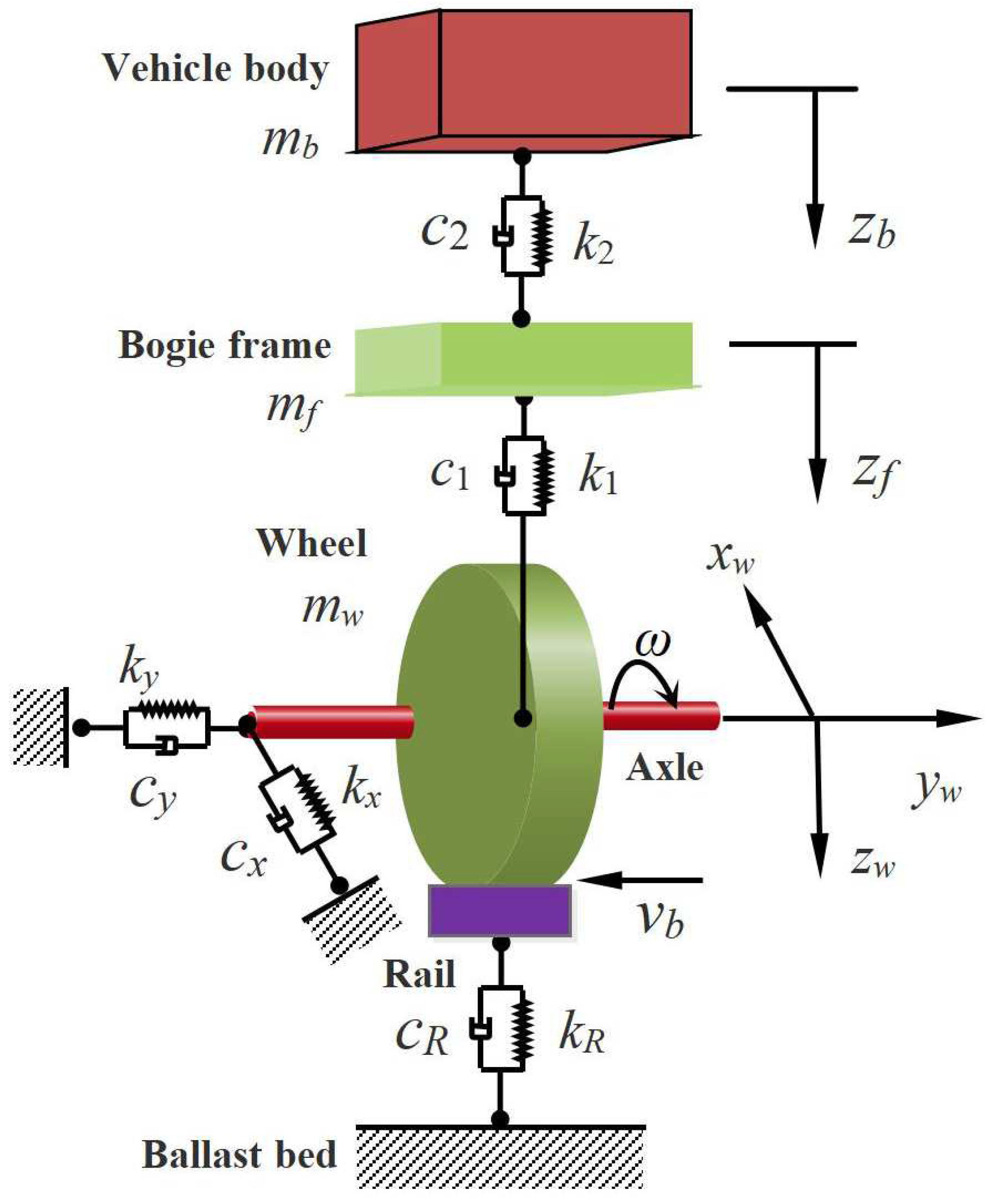
2.1. Rotor Dynamics Model of Wheel–Rail Coupled System

The authors of [23] used the LuGre model and the self-excited vibration theory to develop a single degree of freedom lateral self-excited vibration model of a wheel. The properties of wheel self-excited vibration and the critical condition of Hopf bifurcation were studied, and the process of wheel polygonal wear was simulated.

On the basis of these, in order to study the influencing factors of vertical dynamic load, a lumped-mass model is established by considering the vertical vibration of the car body and frame and the vertical stiffness and damping of the primary and secondary suspension. The rotor dynamics model of the wheel–rail coupled system is shown in Figure 1.

Wheel polygon wear mainly occurs in constant running speed running conditions, using the following assumption:

Assuming that the movement of the left and right wheels has symmetry and considering the symmetry of the wheelset and track structure, 1/8 car body, 1/4 frame, 1/2 wheelset and track are selected as research object, and symmetrical constraints are added to the middle section of the wheelset.

The vehicle operates at a constant running speed in a straight line and 5 degrees of freedom are considered, among which the vehicle body and frame are regarded as rigid bodies and only have vertical degrees of freedom. Wheelsets have longitudinal, lateral, and vertical degrees of freedom.

Because the vertical stiffness of the primary suspension is much lower than the vertical equivalent stiffness of the wheelset, the wheelset flexibility is equivalent to the longitudinal and lateral equivalent stiffness and damping.

The rail is regarded as a massless rigid body and is supported on a rigid ballast by fasteners equivalent to the spring damping element. Due to the large lateral stiffness of the fastener, the influence of the lateral displacement of the rail is neglected, and the vertical support force is provided by the vertical equivalent stiffness and vertical equivalent damping of the fastener.

Consider that the wheelset has an initial polygon of the third order.

The rotor dynamics equation of the wheelset system considering the influence of orbit is established by taking the axle endpoint at the static equilibrium position of the system as the origin of the satellite coordinate system.

$$\{\begin{array}{l}{m}_{\mathrm{b}}{\ddot{z}}_b+c_2({\dot{z}}_b-{\dot{z}}_f)+k_2(z_b-z_f)=0\\ m_f{\ddot{z}}_f+c_2({\dot{z}}_f-{\dot{z}}_b)+k_2(z_f-z_b)+c_1({\dot{z}}_f-{\dot{z}}_w)+k_1(z_f-z_w)=0\\ m_w{\ddot{z}}_w+c_1({\dot{z}}_w-{\dot{z}}_f)+k_1(z_w-z_f)+c_R({\dot{z}}_w-{\dot{z}}_0)+k_R(z_w-z_0)=m_w{e}_w{\omega }^2\cos \omega t-m_{w}g\\ m_w{\ddot{x}}_w+c_x{\dot{x}}_w+k_x{x}_w=m_w{e}_w{\omega }^2\sin \omega t+F_x\\ m_w{\ddot{y}}_w+c_y{\dot{y}}_w+k_y{y}_w=F_y\end{array}$$

(1)

where z_b, z_f, and z_w are the vertical displacement of the car body, frame, and wheel, respectively; x_w and y_w are the longitudinal and lateral displacement of the wheel, respectively. m_w is the mass of the wheel; k_x, k_y, c_x, and c_y are the longitudinal stiffness, longitudinal stiffness, longitudinal damping, and lateral damping; m_f is the frame mass; k₁ and c₁ are the vertical stiffness and damping of the primary suspension; m_b is the body mass; k₂ and c₂ are the vertical stiffness and damping of the secondary suspension; k_R and c_R are the vertical stiffness and damping of the fastener; z₀ is the excitation caused by the initial polygon of the wheel at the wheel–rail contact point; F_x and F_y are the rail contact tangential force; e_w is the eccentricity of the center of mass with respect to the geometric center of the wheel and to the axis of rotation; and ω is the wheel angular running speed.

2.2. Longitudinal Creep Force Model

Creep, which may be classified as longitudinal or lateral creep, is the tangential force occurring between the wheel and rail. Several theoretical models have been developed to address the wheel–rail rolling contact problem, including the Kalker simplified theory, the Polach rolling contact theory, and the empirical formula model [24,25]. The empirical formula describes the dependence of creep forces on creepage in wheel–rail contact, and it includes a saturation feature. Thus, the empirical formula model of changing the friction coefficient [26,27] was used in this work.

$$\{\begin{array}{l}{F}_x={\mu }_x{F}_z\\ {\mu }_x=a{e}^{-b{v}_{rx}}-c{e}^{-d{v}_{rx}}\end{array}$$

(2)

where F_z is the wheel vertical force, which is equal to the static wheel load plus the dynamic vertical force between the wheel and rail. μ_x is the friction coefficient and v_rx is the vertical creepage velocity; a, b, c, and d are the parameters reflecting the contact state of the wheel and rail, which can be fitted by the measured data according to the specific situation of the wheel and the rail contact surface. a = 0.53, b = 0.43, c = 0.53, and d = 8.64 [26], respectively.

Because the wheels have non-cylindrical treads, the wheelset is in hunting during operation. At the same time, the wheel’s structural flexibility affects wheel–rail contact, the impact the wheel’s structural flexibility during wheel–rail contact is taken into account in the model, and the flexible contact between the wheelset and rail will produce creep. The effects of the above two points are considered with an effective relative yaw angle ψ. Then, the actual running speed of the wheelset is $v=\omega R\cos \psi$. When not considering the wheelset as flexible, the wheelset longitudinal creepage velocity is $\Delta v=\omega R-\omega R\cos \psi$. When considering the wheel as flexible, the wheelset will produce flexible vibration, and its creepage velocity is Equation (3).

$$v_{rx}=\Delta v-{\dot{x}}_w=\omega R(1-\cos \psi )-{\dot{x}}_w$$

(3)

where v_rx and ${\dot{x}}_w$ are the longitudinal creep and longitudinal vibration speed of the axle and wheel, respectively and, R is the wheel radius.

2.3. Lateral Creep Force Model

According to previous study findings by the author’s team [22,23], the lateral vibration of a wheel is more comparable to dry friction vibration. There are two types of frequently used friction models today [28]. North proposed a self-excited vibration caused by friction forces with a constant friction coefficient μ, whereas Murakami et al. [28] proposed a mechanism that combines the dμ/dv < 0 theory with Spurrs’ sprag-slip theory. In this study, we present a dynamic friction model [29]. The model treats the innumerable bristles between the two items composing the dry friction pair as springs, and the friction force increases as these springs bend elastically. When the two objects have a relative speed, the bristles will initially exhibit the properties of a spring, such as elastic deformation and static friction force; however, as the elastic deformation increases, the bristles will slip relative to the contact surface, resulting in a dynamic friction force. The procedure accurately represents the negative slope of the dynamic friction force. As a result, the lateral translation of the wheels and rails is converted into the pulley drive, as illustrated in Figure 2, and the lateral creep force between the wheels and rails may be described as follows:

$$\{\begin{array}{l}{F}_y={\sigma }_{0}s+{\sigma }_1\dot{s}+{\sigma }_2{v}_{ry}\\ \dot{s}=v_{ry}-{\displaystyle \frac{{\sigma }_{0}s}{F_{vr}}}\left|v_{ry}\right|\\ v_{ry}=\omega R\sin \psi -{\dot{y}}_w\\ F_{vr}={\mu }_y{F}_z\\ {\mu }_y={\mu }_s+({\mu }_m-{\mu }_s){\mathrm{e}}^{-|v_{ry}/v_s{|}^{\varphi }}\end{array}$$

(4)

where σ₀ and σ₁ are the stiffness and damping coefficient, respectively. σ₂ is the relative viscous damping coefficient, and the wheel–rail viscosity effect on the high-quality straight line is negligible, that is σ₂ = 0. s is the elastic deformation of the brush, v_ry is the lateral creep velocity of the wheel and rail, v_s and φ are the Stribeck velocity and the Stribeck index in the steady state friction properties, and μ_m and μ_s are the maximum static and sliding friction coefficients, respectively.

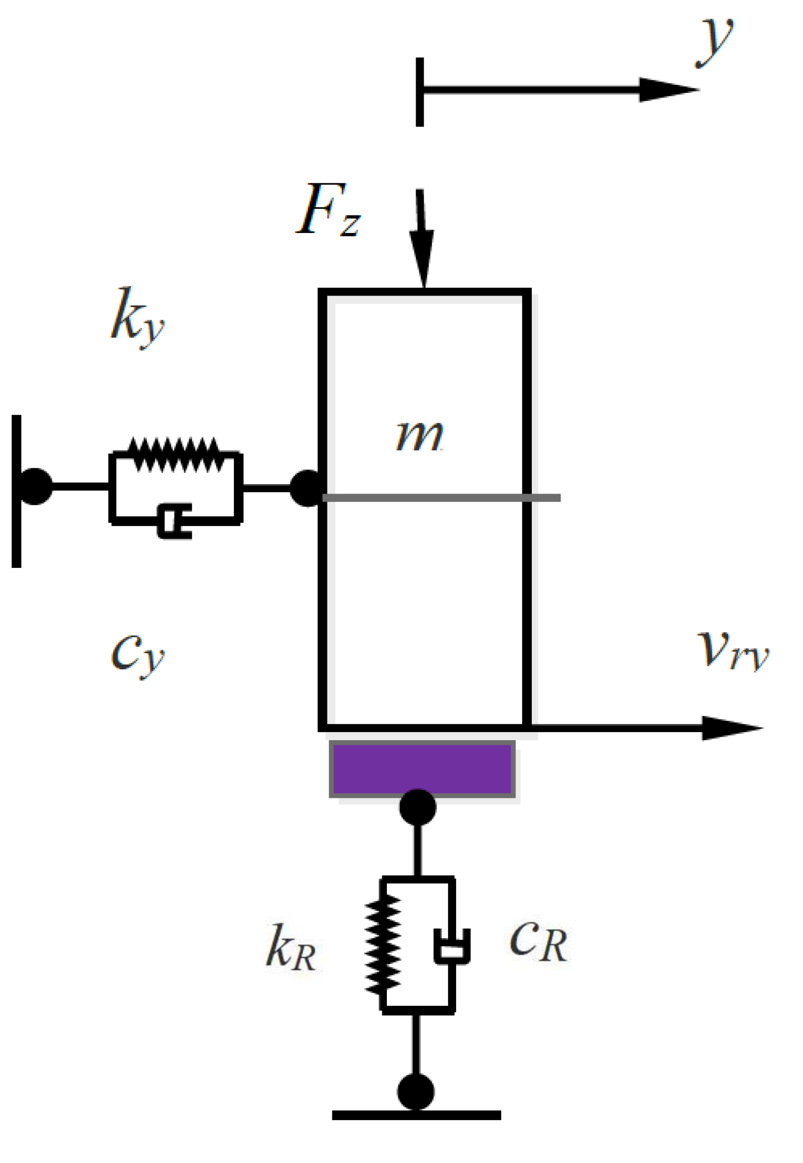
2.4. Vertical Force Model

Considering the fastener stiffness and damping, the wheel initial polygon z₀, the vertical force of the wheel and rail can be expressed as follows:

$$\{\begin{array}{l}{F}_z=P_0+c_R({\dot{z}}_w-{\dot{z}}_0)+k_R(z_w-z_0)\\ z_0=A_0\sin (n_0\omega t+\varphi )\end{array}$$

(5)

where P₀ is the wheel load, and A₀, n_0, and φ₀ are the amplitude, order, and phase angle of the initial polygon, respectively.

Before solving the aforesaid model, it is important to identify the equivalent stiffness and damping of the wheelset, which are associated with a certain mode of the flexible wheelset.

2.5. Lateral Self-Excited Vibration Analysis

Regardless of the geometric relationship of wheel–rail contact or the rolling contact theory, Morys [30] suggested that lateral slip in wheel–rail contact is the primary source of polygonal wear. This article investigates wheel polygonal wear under lateral vibration of a wheel–rail system.

2.5.1. The Mechanism of Self-Excitation Vibration

This research examines the vibration mechanism of the wheel-rail coupled system in terms of energy. As we only consider the wear of the lateral creep force, the energy equation of the wheel-rail system may be found by combining Equation (4) and 5th equation multiply $\mathrm{d}{y}_w={\dot{y}}_w\mathrm{d}t$ in Equation (1).

$$\mathrm{d}({\displaystyle \frac{1}{2}}{m}_w{\dot{y}}_w^2+{\displaystyle \frac{1}{2}}{k}_w{y}_w^2)+c_y{\dot{y}}_w^{2}dt-({\sigma }_{0}s+{\sigma }_1\dot{s}){\dot{y}}_{w}dt=0$$

(6)

Integral from 0~τ Equation (6)

$${\displaystyle \frac{1}{2}}{m}_w{\dot{y}}_{w\tau }^2+{\displaystyle \frac{1}{2}}{k}_w{y}_{w\tau }^2={\displaystyle \frac{1}{2}}{m}_w{\dot{y}}_{w0}^2+{\displaystyle \frac{1}{2}}{k}_w{y}_{w0}^2-{\displaystyle {\int }_0^{\tau }{c}_y{\dot{y}}_w^{2}dt}+{\displaystyle {\int }_0^{\tau }({\sigma }_{0}s+{\sigma }_1\dot{s}){\dot{y}}_{w}dt}$$

(7)

Term 1 on the left side of Equation (7) is the kinetic energy of the wheel–rail system at time τ: T. Term 2 is the elastic potential energy at time τ: V. Term 1 on the right is the kinetic energy at time 0: T₀. Term 2 is the elastic potential energy at time 0: V₀. Term 3 is the Rayleigh dissipation function: D. Term 4 is the creep force work: W_F. This can be seen in Equation (7):

$$T+V=T_0+V_0-D+W_F$$

(8)

According to Equation (8), the wheel–rail system is a non-conservative dissipative system, with an initial energy of T₀ + V₀ before the initial disturbance; after the initial disturbance, its energy changes because the Rayleigh dissipation function term D remains positive and contributes to energy dissipation. According to Equation (4), the lateral creep force F_y contains the stiffness term and the damping term, which dissipate the energy of the wheel–rail system, and the stiffness term conveys the vibration energy of the wheel–rail system. When the dissipated energy is larger than the input energy, the wheel vibration converges to the equilibrium position. When the dissipation energy is less than the input energy, the wheel’s self-excited vibration is activated, and the wheel is stable in certain limit cycles. The magnitude of the lateral creep velocity depends on the direction and amplitude of the lateral vibration of the wheelset at the current moment and directly affects the magnitude of the lateral creep force and its distribution in the friction coefficient curve; the lateral creep force at the current moment affects the running speed of the wheels at the next moment. Through the creepage velocity feedback mechanism, the size of the damping term of the creep force is changed to affect the relative relationship between the input energy and the dissipation energy, and the original wheelset’s forward energy is converted into the wheelset’s lateral vibration energy, which is the energy source of the self-excited vibration of the wheelset. It can be seen that the lateral self-excited vibration caused by the feedback mechanism of the lateral creepage velocity is a necessary condition for wheel polygonal wear.

2.5.2. Self-Excited Vibration Stability Condition

By transforming the equations of motion given by Equation (1) into the state–space representation, the following equations are obtained.

$$\{\begin{array}{l}{\dot{y}}_1=y_2\\ {\dot{y}}_2=-[c_2(y_2-y_4)+k_2(y_1-y_3)]/m_b\\ {\dot{y}}_3=y_4\\ {\dot{y}}_4=-[c_2(y_4-y_2)+k_2(y_3-y_1)+c_1(y_4-y_6)+k_1(y_3-y_5)]/m_f\\ {\dot{y}}_5=y_6\\ {\dot{y}}_6=-[c_1(y_6-y_4)+k_1(y_5-y_3)+c_R(y_6-{\dot{z}}_0)+k_R(y_5-z_0)-m_w{e}_w{\omega }^2\cos \omega t]/m_w\\ {\dot{y}}_7=y_8\\ {\dot{y}}_8=-[c_x{y}_8+k_x{y}_7-m_w{e}_w{\omega }^2\sin \omega t-F_x]/m_w\\ {\dot{y}}_9=y_{10}\\ {\dot{y}}_{10}=-[c_y{y}_{10}+k_y{y}_9-F_y]/m_w\end{array}$$

(9)

Expressed in matrix form

$$\dot{q}=Aq+Bu$$

(10)

where A is the Jacobi matrix of the system state variable, q is the system state vector, $q={[y_1,y_2,\dots ,y_{10}]}^{\mathrm{T}}$, B is the system input variable matrix, and u is the input vector, $u={[u_1,u_2,\dots ,u_{10}]}^{\mathrm{T}}$.

When the system is in equilibrium, it satisfies ${\dot{y}}_i=0,(i=1,2,\dots ,10)$. Substituting this condition into Equation (9), the equilibrium point and the corresponding longitudinal creep coefficient μ_x0 and the lateral creep coefficient μ_y0 can be solved. The Taylor expansion is carried out for the nonlinear functions F_x and F_y, whereby the equilibrium state is used as the reference state and only the linear term is taken into account, and by taking the linear term substitution of Equation (9), the Jacobi matrix of the corresponding equation of state of the linear system is as follows:

$$A=\left[\begin{array}{cccccccccc}0& 1& 0& 0& 0& 0& 0& 0& 0& 0\\ -{\displaystyle \frac{k_2}{m_b}}& -{\displaystyle \frac{c_2}{m_b}}& {\displaystyle \frac{k_2}{m_b}}& {\displaystyle \frac{c_2}{m_b}}& 0& 0& 0& 0& 0& 0\\ 0& 0& 0& 1& 0& 0& 0& 0& 0& 0\\ {\displaystyle \frac{k_2}{m_f}}& {\displaystyle \frac{c_2}{m_f}}& -{\displaystyle \frac{k_2+k_1}{m_f}}& -{\displaystyle \frac{c_1+c_2}{m_f}}& {\displaystyle \frac{k_1}{m_f}}& {\displaystyle \frac{c_1}{m_f}}& 0& 0& 0& 0\\ 0& 0& 0& 0& 0& 1& 0& 0& 0& 0\\ 0& 0& {\displaystyle \frac{k_1}{m_w}}& {\displaystyle \frac{c_1}{m_w}}& -{\displaystyle \frac{k_1+k_R}{m_w}}& -{\displaystyle \frac{c_1+c_R}{m_w}}& 0& 0& 0& 0\\ 0& 0& 0& 0& 0& 0& 0& 1& 0& 0\\ 0& 0& 0& 0& {\mu }_{x0}{\displaystyle \frac{k_R}{m_w}}& {\mu }_{x0}{\displaystyle \frac{c_R}{m_w}}& -{\displaystyle \frac{k_x}{m_w}}& -{\displaystyle \frac{c_x}{m_w}}& 0& 0\\ 0& 0& 0& 0& 0& 0& 0& 0& 0& 1\\ 0& 0& 0& 0& {\mu }_{y0}{\displaystyle \frac{k_R}{m_w}}& {\mu }_{y0}{\displaystyle \frac{c_R}{m_w}}& 0& 0& -{\displaystyle \frac{k_y}{m_w}}& -{\displaystyle \frac{c_y}{m_w}}\end{array}\right]$$

(11)

The characteristic root equation of the matrix is as follows:

$$\left|\lambda E-A\right|=0$$

(12)

$${\lambda }^{10}+a_1{\lambda }^9+a_2{\lambda }^8+\dots +a_9\lambda +a_{10}=0$$

(13)

According to the Routh–Hurwitz criterion, the determinants of the Routh–Hurwitz composed of coefficients of Equation (14) are all greater than zero, all roots of the characteristic equation have negative real parts, and the system is asymptotically stable. The system Hopf bifurcation conditions is as follows:

$$\left|D\right|=\left|\begin{array}{cccccccc}{a}_1& 1& 0& 0& 0& 0& \dots & 0\\ a_3& a_2& a_1& 1& 0& 0& \dots & 0\\ a_5& a_4& a_3& a_2& a_1& 1& \dots & 0\\ \dots & \dots & \dots & \dots & \dots & \dots & \dots & .\\ 0& 0& 0& 0& 0& 0& \dots & a_{10}\end{array}\right|=0$$

(14)

where D is the coefficients of the characteristic equation arranged in a square matrix of the 10th order. Combinied with Equation (11), the parameters affecting system stability mainly include the mass, stiffness, damping, and friction coefficients of each part of the wheel–rail system.

3. Wheel Polygonal Wear Model

The wheel circumferential profile z₀ is determined by the radial wear of the wheel:

$$z_0(t)=z_0(t-T)-\Delta r(t)$$

(15)

where T is the period of the wheel rotation and the period for one rotation should be $T={\displaystyle \frac{\pi D}{v_0}}$. $\Delta r(t)$ is the wheel wear depth.

The Archard model [31] and the wear work model [32] are the two most often used wheel material wear models for the prediction of polygonal wear. Both wheel polygonal evolution patterns are essentially the same, according to studies, although the latter findings are more accurate and have greater efficiency [33]. As a result, the Specht wear work model was used in this study, which makes the assumption that the mass loss due to wear Δm is proportional to the wear work at the point of wheel–rail contact.

$$\Delta m=K_w\cdot W_w$$

(16)

where K_w is the wear work coefficient.

$$K_w=\{\begin{array}{l}\begin{array}{cc}3\cdot {10}^{-9}\mathrm{kg}/\mathrm{J}& W_w\le 4\cdot {10}^6{\mathrm{J}/\mathrm{m}}^2\end{array}\\ \begin{array}{cc}2\cdot {10}^{-8}\mathrm{kg}/\mathrm{J}& W_w>4\cdot {10}^6{\mathrm{J}/\mathrm{m}}^2\end{array}\end{array}$$

(17)

In the process of wheel creep, frictional work is the product of tangential force at the contact point and the sliding distance of the wheel. In this paper, only the lateral wear which is dissipated due to lateral creepage in the contact was considered, so W_w can be expressed as follows:

$$W_w={\displaystyle {\int }_0^l{\tau }_{y}d{s}_y}=F_y{s}_w$$

(18)

where l is the contact length, τ_y is the lateral force, ds_y is the lateral sliding distance, and s_w is the wheel–rail relative sliding distance.

Δm is equal to the product of the wear depth Δr, the wear area A_w, and the material density ρ, that is, $\Delta m=\rho \cdot A_w\cdot \Delta r$. Combined with the formula from Equations (16) and (18), the calculation equation of the wheel wear depth Δr is as follows:

$$\begin{array}{l}\Delta r={\displaystyle \frac{\Delta m}{\rho \cdot A_w}}={\displaystyle \frac{K_w\cdot W_w}{\rho \cdot A_w}}={\displaystyle \frac{K_w\cdot F_y\cdot s_w}{\rho \cdot b_w\cdot s_w}}\\ ={\displaystyle \frac{K_w}{\rho \cdot b_w}}{F}_y\end{array}$$

(19)

where b_w is the average width of the wear zone.

As can be seen from Equation (19), wheel wear is related to the lateral creep force. When the lateral creep force F_y is periodically changed according to a certain frequency, the wear depth Δr changes periodically, resulting in polygonal wear. When the lateral creep force F_y is at its maximum, peak wear occurs only once during a cycle of lateral vibration of the wheel. If the lateral vibration frequency of the wheel is f_y, the time interval of two instances of adjacent wear peak consumption is 1/f_y, the wheel rotation frequency is f₁, and the wheel rotation period is 1/f₁. The number of peak wear values (order) n occurring in a circle of wheel rotation is as follows:

$$n={\displaystyle \frac{f_y}{f_1}}={\displaystyle \frac{2\pi f_y}{\omega }}$$

(20)

4. The Numerical Simulation

Table 1. Calculation parameters of EMU vehicles.

The Parameter Name	Parameter Values
Mass of car body mb/kg	40,384
Mass of bogie frame mf/kg	2056
Mass of wheelset mw/kg	1627
Secondary stiffness k2/(MN·m−1)	0.80
Secondary damping c2/(kN·s·m−1)	30
Primary stiffness k1/(MN·m−1)	2.08
Primary damping c1/(kN·s·m−1)	20
Wheel diameter D/mm	920
Wheel load P0/kN	80
Fastener stiffness kR/(MN·m−1)	25
Fastener damping cR/(kN·s·m−1)	15
Eccentricity of wheelset mass ew/(μm)	1.00

shows the CRH₃ EMU parameters, along with the LuGre model parameters, σ₀ = 4.05 × 10⁶ N·m⁻¹, σ₁ = 3.33 × 10⁵ N.s·m⁻¹, v_s = 0.2 m·s⁻¹, φ = 0.9, μ_m = 0.5, μ_s = 0.25, and ψ = 0.3°. This is based on the results of the authors’ previous research on the single-degree-of-freedom model to determine wheelset flexibility [22,23].

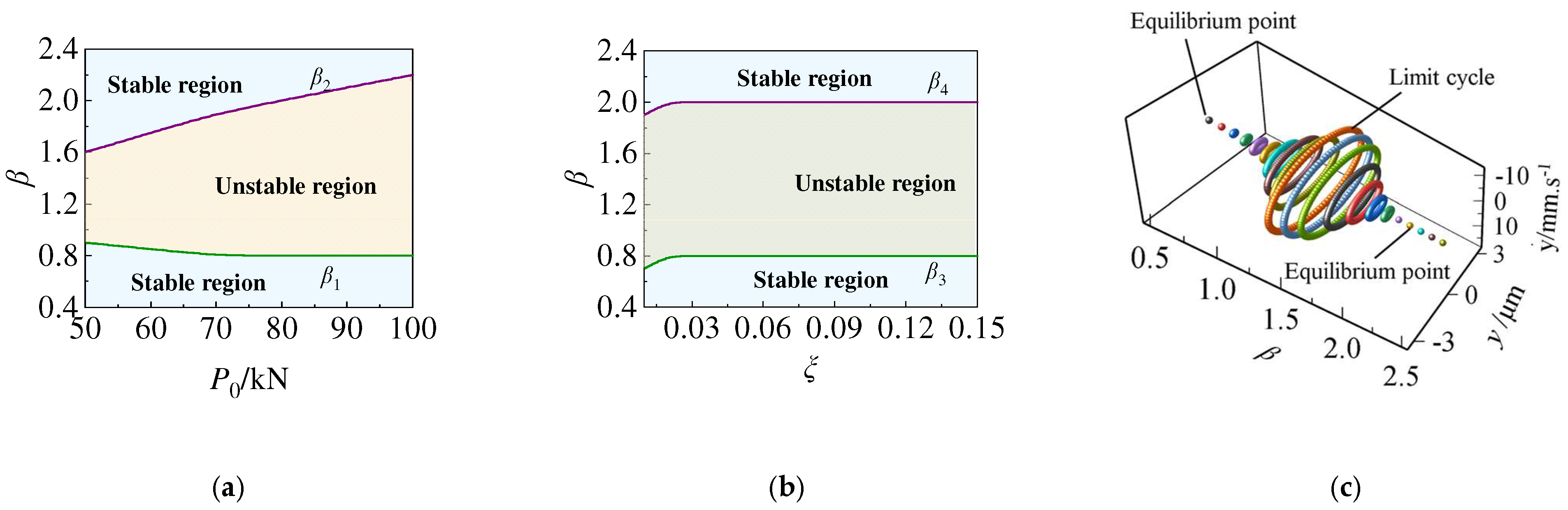
4.1. Stability Analysis

It is difficult to obtain the analytical solution of the lateral self-excited vibration condition by Equation (14), reference Equations (11) and (14), and Equation (1) for numerical simulation. Since the train running speed is much larger than the relative speed at the contact point of the wheel and rail, the speed ratio is the ratio of the train running speed normalized to the relative speed at 250 km/h, As a result, the speed ratio is β = v/(250v_s). The damping ratio is the lateral damping c_y divided by the critical damping c_c($c_c=2\sqrt{m_w{k}_y}$)_, that is, $\xi =c_y/(2\sqrt{m_w{k}_y})$. Figure 3 shows the stability boundaries and stability domains for the solutions, which are obtained by numerically solving Equation (1), displayed in the P₀-β map and in the ξ-β map.

The critical lines β₁ and β₂ of the parameters divide the parameter domain (P₀, β) into three parts, as shown in Figure 3a: the region of β < β₁ and β > β₂ is stable; there is no periodic orbit in the system vibration; the region of β₁ < β < β₂ is unstable, and periodic orbit exists. As the wheel load P₀ increases, β₁ decreases slightly, and β₂ increases, indicating that as the wheel load increases, the unstable region expands. The parameter domain (ξ, β) is divided into three sections by the critical lines β₃ and β_4, as shown in Figure 3b: the regions of β < β₃ and β > β₄ are stable, while the region of β₃ < β < β₄ is unstable. With the increase in the damping ratio, the values of β₃ and β₄ are constant.

As observed in Figure 3c, when P₀ = 80 kN, the lateral vibration of the wheelset is the stable spiral at a slow running speed. When the running speed increases to β₁, the lateral vibration instability becomes a limit cycle, and the amplitude of the limit cycle first increases and then decreases; when the running speed increases to β₂, the lateral vibration becomes the focus of stability again. This shows that there are balance points and limit cycle vibrations when the running speed changes, and the limit cycle amplitude changes with the running speed. This bifurcation phenomenon is consistent with the conclusion of the authors’ previous research [23] on the single degree of freedom model, which verifies the feasibility of the model established in this paper. To identify the vibration characteristics of the system at the critical point, the changes in the parameters are analyzed below.

4.2. Parameter Effects

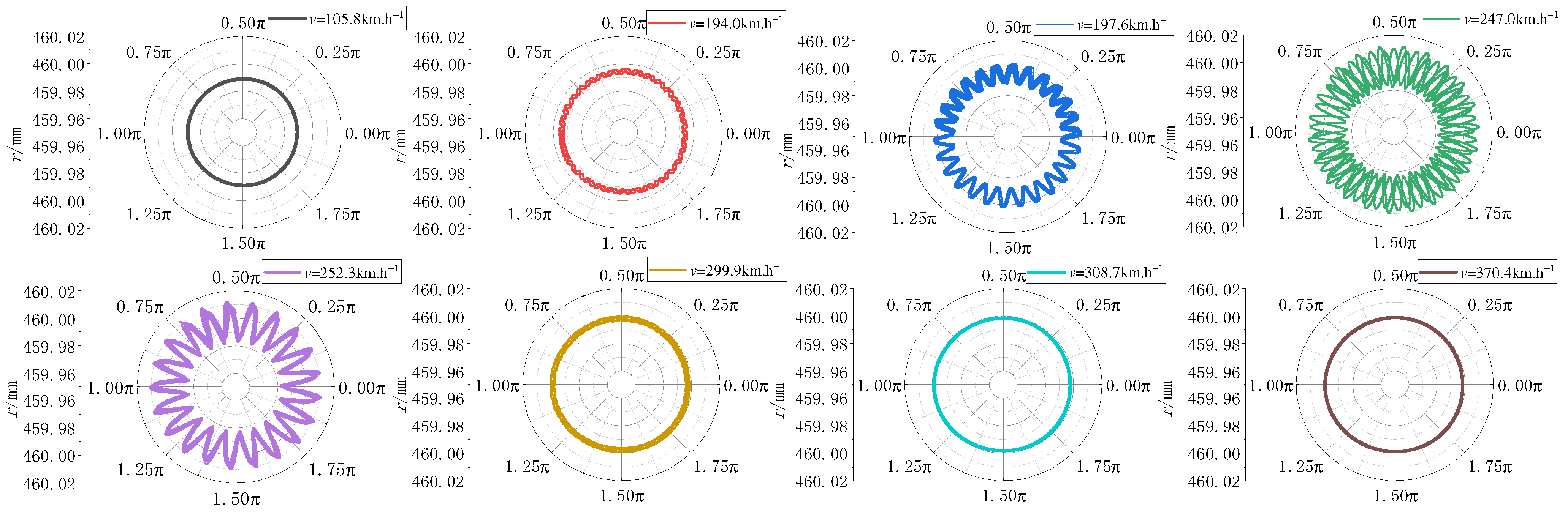
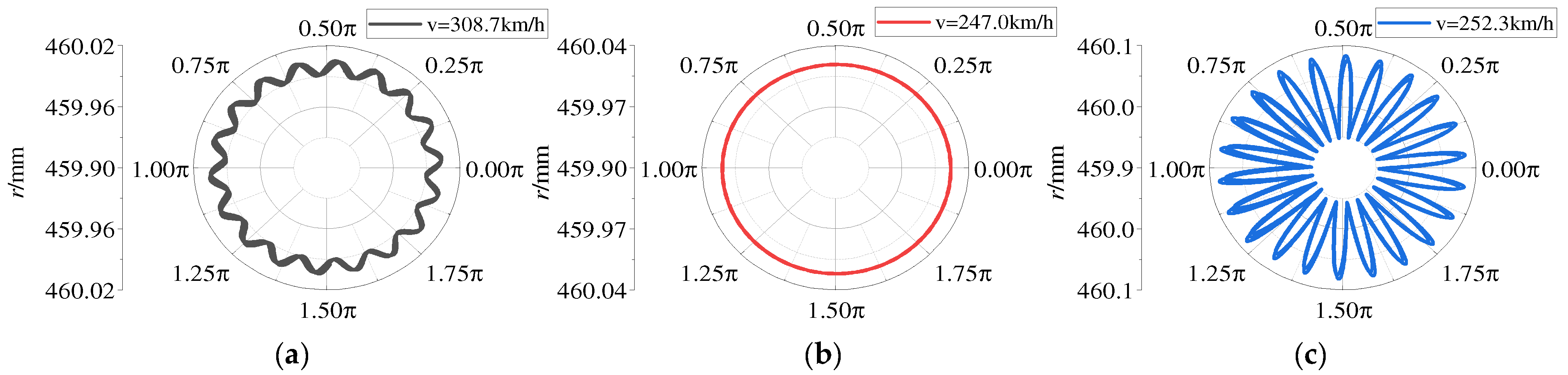
4.2.1. The Effect of the Running Speed

Taking 0.5 ≤ β ≤ 2.5 and P₀ = 80 kN, vibration characteristics and wheel wear characteristics at different rotational speeds were studied, as shown in Figure 4.

The running speed bifurcation diagram in Figure 4a demonstrates that the wheel does not generate self-excited vibration for β < 0.6, and the bifurcation diagram is a straight line. When the running speed reaches β = 0.6, the system becomes unstable, the supercritical Hopf bifurcation takes place, and self-excited vibration is produced by the wheel. The amplitude of the limit cycle reaches its greatest value at β = 1.4. β = 2.1, the system has a subcritical Hopf bifurcation and is stable again, and the wheel does not generate self-excited vibration.

As can be seen from Figure 4b, the lateral self-excited vibration response of the wheel in the instability region (0.6 < β < 2.1) contains three frequency components: the wheel rotation frequency f₁ caused by the eccentricity of the wheelset mass, the frequency 3× caused by the initial wheel polygon of the 3rd order, and the main vibration frequency f₂ = 586.2 Hz which is independent of the running speed. This phenomenon indicates that the lateral vibration of the wheel is affected by vertical excitation, and the characteristic of “fixed frequency” is obvious, which is consistent with the conclusion of the reference [23] and verifies the feasibility of the model established in this paper.

Figure 4c of the wheel wear characteristics shows that uniform wear on the wheel circumference occurs when self-excited vibration does not occur in the stable region β = 2.2; however, obvious harmonic wear appears in the instability regions β = 1.2 and β = 1.4, indicating that lateral self-excited vibration is the primary contributor to wheel polygonal wear.

4.2.2. The Effect of the Wheelset Flexibility

In order to investigate the influence of the wheelset’s structural dynamics, the lateral damping c_y and the lateral stiffness k_y are varied within the ranges of 1.0 kN·s·m⁻¹ ≤ c_y ≤ 20.0 kN·s·m⁻¹ and 2250 MN·m⁻¹ ≤ k_y ≤6570 MN·m^−1, respectively. For this investigation, the constant values β = 1.6 and P₀ = 80 kN are chosen.

Figure 5a demonstrates that the system exhibits supercritical Hopf bifurcation instability at c_y = 1.0 kN·s·m⁻¹ lateral damping. Figure 5b shows that when the damping coefficient rises, the fixed frequency remains constant while the amplitude increases, which makes the amplitude gradually increase and the polygon order does not change, as shown in Figure 5c. It is clear that the amplitude of the wheel higher order polygon is influenced by the lateral damping of the wheelset.

It can be seen from Figure 6a that the system first becomes unstable through the supercritical Hopf bifurcation and then becomes stable through the subcritical Hopf bifurcation by the influence of lateral stiffness. With the increase in lateral stiffness, the fixed frequency gradually increases, and the amplitude shows an overall downward trend, as shown in Figure 6b. The order of the wheel polygon gradually increases and the amplitude gradually decreases, as shown in Figure 6c. It can be seen that the lateral stiffness of the wheelset is the main factor affecting the order of the polygon.

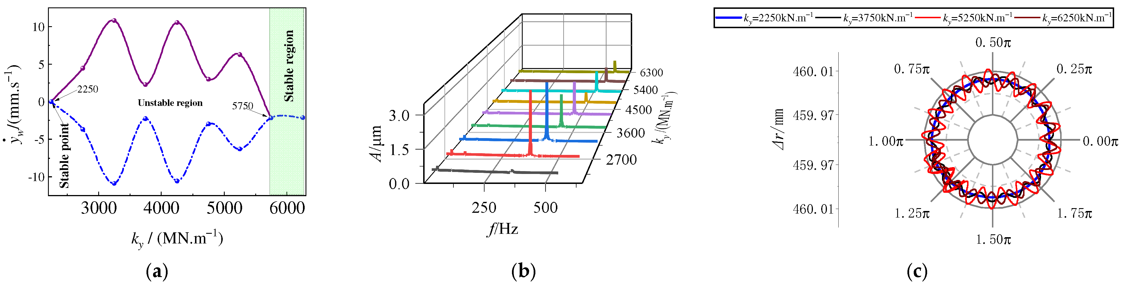
4.2.3. The Effect of Primary Suspension Parameters

We take into account β = 1.6, the wheel load as P₀ = 80 kN, and investigating the vibration characteristics at the vertical stiffness k₁ = 7 kN·m⁻¹, 70 kN·m⁻¹, 700 kN·m⁻¹, 7000 kN·m⁻¹ and the vertical damping c₁ = 5 kN·s·m⁻¹, 10 kN·s·m⁻¹, 20 kN·s·m⁻¹, 30 kN·s·m⁻¹, 40 kN·s·m⁻¹, 50 kN·s·m⁻¹.

Figure 7a,c show that the primary stiffness and damping have almost no effect on the fixed frequency and its amplitude, and then have little effect on the wheel polygon order and amplitude (seen in Figure 7b,d). Therefore, polygonal wear is not sensitive to the parameters k1 and c1, so the influence of the parameters on the polygonal wear can be neglected.

4.2.4. The Effect of the Rail

We take into account β = 1.6, P₀ = 80 kN, and investigate the vibration characteristics at the fastener stiffness k_R = 0.2 MN·m⁻¹, 2.0 MN·m⁻¹, 20 MN·m⁻¹, and 200 MN·m⁻¹, as well as the fastener damping c_R = 5.0 kN·s·m⁻¹, 10.0 kN·s·m⁻¹, 20.0 kN·s·m⁻¹, 30.0 kN·s·m⁻¹, 40.0 kN·s·m⁻¹.

The fastener stiffness k_R has no effect on the fixed frequency, as shown in Figure 8a. The response amplitude of the initial polygon gradually increases with the increase in fastener stiffness, even exceeding the amplitude of the fixed frequency, and the initial polygonal wear evolution is also very visible (see Figure 8b). Furthermore, the fastener damping c_R has little effect on both the wheel polygon order and amplitude, as shown in Figure 8c,d. It is clear that the influence of rail characteristics on polygonal wear is primarily due to fastener stiffness, which supports the conclusion that the rail mode is an important factor in wheel polygonal wear.

5. Analysis of Wheel Polygonal Wear Evolution

5.1. Evolution of Wheel Polygonal Wear at Constant Running Speed

The generation of wheel polygonal wear is the result of the accumulation of wheel tread wear, and thus the evolution of wheel polygonal wear in the range of the self-excited vibration running speed should be studied. The wear caused by rail irregularity can be regarded as stable uniform wear when a new wheel rolls on a high-quality straight line at a constant running speed. At this moment, the only factor that causes wheel polygonal wear with a specific frequency change is the lateral self-excited vibration of the wheel. The wheel polygon order is the ratio of the wheelset rotation frequency to the self-excited vibration frequency which can be calculated by Equation (20). The wheel polygonal wear characteristics are drawn for running speeds of v = 194.0 km/h, 197.6 km/h, 247.0 km/h, 252.3 km/h, 299.9 km/h, and 308.7 km/h using the results of the running speed bifurcation analysis, as shown in Figure 9.

Figure 9 shows that at the running speeds of v = 105.8 km/h and 370.4 km/h, the system does not have lateral self-excited vibration, and the wheel shows uniform wear on the whole circumference. The system causes lateral self-excited vibration at the running speeds of v = 194.0 km/h, 247 km/h, and 299.9 km/h, but the generated wear cannot be accumulated at the same circumferential position and the wheel shows the superposition of multiple harmonic wear. At the running speeds of v = 197.6 km/h, 252.3 km/h, and 308.7 km/h, the lateral self-excited vibration of the system generates cumulative wear at the same circumferential position and evolves into obvious polygonal wear, and the polygon order is the ratio of the fixed frequency (586.2 Hz) to the rotating frequency. When running at a constant running speed, the evolution of wheel polygonal wear exhibits “integer division” characteristics. The research findings support the theoretical analysis conclusion that wheel polygonal wear has “constant frequency and integer division” [20].

The worn-out limit diameter is 830 mm, and the new wheel diameter is 920 mm. Currently, the high-speed EMU operates at a constant running speed of 300 km/h. According to the above principle of “fixed frequency and integral division”, the wheel diameter corresponding to the wheel rotating frequency that can divide the fixed frequency and can be calculated by Equation (20) as 915.1 mm (20 times) and 869.4 mm (19 times). It can be seen that there are two high-incidence periods of wheel polygon wear during the whole life cycle of the wheel, which is consistent with the field measurement results [3]. This conclusion can be used as a theoretical basis for formulating the timing and cycle of wheel reprofiling.

5.2. Evolution of Wheel Polygonal Wear at Variable Running Speed Operations

The high-speed EMU has two operating levels of 300 km/h and 250 km/h. This section discusses how wheel polygonal wear evolves under the condition of changing the running speed level.

The 18th-order wheel polygon is generated after 500 cycles at the running speed v = 308.7 km/h in the first stage, as shown in Figure 10a. The 18th-order polygon generated in the first stage serves as the initial polygon in the second stage, and the wheel polygonal wear characteristics are generated after another 500 cycles at the running speed v = 247.0 km/h (non-integer division) and the running speed v = 252.3 km/h (n = 22), respectively, as shown in Figure 10b,c.

Figure 10b,c shows that when the running speed is reduced to v = 247.0 km/h, the original 18th-order polygon gradually disappears and does not evolve into obvious-order wheel polygonal wear. Whereas, when the running speed is reduced to v = 252.3 km/h, the original 18th-order polygon gradually evolves into a 22nd-order polygon. It can be seen that the evolution of wheel polygonal wear still follows the wear law of “integer division” with a change in running speeds, and that wheel polygonal wear can only be effectively suppressed by selecting a reasonable running speed value.

6. Conclusions

A wheelset system’s rotor dynamics model and wheel polygon wear model are developed with the track’s influence and the effect of the wheelset rotation in mind. The system’s lateral self-excited vibration stability is examined. Analyzed are the parameters’ effects and the circumstances for the wheel polygon’s generation and evolution mechanism. The primary research findings are listed below.

The Hopf bifurcation region for the wheelset flexibility parameters and rotational speed is determined.

The lateral self-excited vibration caused by the lateral creepage velocity feedback mechanism is a necessary requirement for polygonal wear on wheels.

The development of wheel polygonal wear demonstrates clear “fixed frequency” features. The fixed frequency is mostly influenced by the flexibility of the wheelset and is virtually completely independent of the suspension parameters. The sequence of wheel polygonal wear is mostly governed by the wheelset’s lateral stiffness and rotating speed, whereas the amplitude is primarily determined by the wheel load, the lateral damping of the wheelset, and fastener stiffness.

The progression of wheel polygonal wear exhibits “integer division” characteristics. When the wheel is running at a steady speed, there are many phases of high polygonal wear before the wheel diameter wear reaches its maximum. When operating at different speeds, wheel polygonal wear still adheres to the “integer division” rule.

To simplify the calculation and illustrate the mechanism of wear generation and evolution, this study assumes that the left and right wheels move symmetrically when building the model and take up half of the wheel–rail. However, in order to analyze the wheelset hunting motion and rotation motion, we must first develop a comprehensive coupling model.

References

1. Nielsen, J.C.O.; Lunden, R.; Johansson, A. Train-track interaction and mechanisms of irregular wear on wheel and rail surfaces. Veh. Syst. Dyn. 2003, 40, 3–54. [Google Scholar] [CrossRef]
2. Tao, G.; Wen, Z.; Jin, X.; Yang, X. Polygonisation of railway wheels: A critical review. Rail. Eng. Sci. 2020, 28, 317–345. [Google Scholar] [CrossRef]
3. Jin, X.; Wu, Y.; Liang, S.; Wen, Z.F.; Wu, X.W.; Wang, P. Characteristics, mechanism, influences and countermeasures of polygonal wear of high-speed train wheels. J. Mech. Eng. 2020, 56, 118–136. (In Chinese) [Google Scholar]
4. Nielsen, J.C.O.; Johansson, A. Out-of-round railway wheels—A literature survey. Proc. Inst. Mech. Eng. F J. Rail Rapid. Transit. 2000, 214, 79–91. [Google Scholar] [CrossRef]
5. Johansson, A.; Nielsen, J.C.O. Out-of-round railway wheels—Wheel-rail contact forces and track response derived from field tests and numerical simulations. Proc. Inst. Mech. Eng. F J. Rail Rapid. Transit. 2003, 217, 135–146. [Google Scholar] [CrossRef]
6. Wang, P.; Tao, G.; Yang, X.; Xie, C.; Li, W.; Wen, Z. Analysis of Polygonal Wear Characteristics of Chinese High-Speed Train Wheels. J. Southwest Jiaotong Univ. 2023, 58, 1357–1365. (In Chinese). Available online: http://kns.cnki.net/kcms/detail/51.1277.U.20211124.1532.002.html (accessed on 3 June 2024). (In Chinese).
7. Wu, Y.; Wang, J.; Liu, M.; Jin, X.; Hu, X.; Xiao, X.; Wen, Z. Polygonal wear mechanism of high-speed wheels based on full-size wheel-rail roller test rig. Wear 2022, 494–495, 204234. [Google Scholar] [CrossRef]
8. Jin, X.; Wu, L.; Fang, J.; Zhong, S.; Ling, L. An investigation into the mechanism of the polygonal wear of metro train wheels and its effect on the dynamic behaviour of a wheel/rail system. Veh. Syst. Dyn. 2012, 50, 1817–1834. [Google Scholar] [CrossRef]
9. Tao, G.; Xie, C.; Wang, H.; Yang, X.; Ding, C.; Wen, Z. An investigation into the mechanism of high-order polygonal wear of metro train wheels and its mitigation measures. Veh. Syst. Dyn. 2020, 59, 1557–1572. [Google Scholar] [CrossRef]
10. Yang, X.; Tao, G.; Wen, Z. Causes and evolution of asymmetric polygonal wear of metro train wheelsets. Wear 2023, 530–531, 205036. [Google Scholar] [CrossRef]
11. Fröhling, R.; Spangenberg, U.; Reitmann, E. Root cause analysis of locomotive wheel tread polygonization. Wear 2019, 432–433, 102911. [Google Scholar] [CrossRef]
12. Spangenberg, U. Variable frequency drive harmonics and inter harmonics exciting axle torsional vibration resulting in railway wheel polygonization. Veh. Syst. Dyn. 2019, 58, 404–424. [Google Scholar] [CrossRef]
13. Wu, X.; Liang, S.; Chi, M. An investigation of rocking derailment of railway vehicles under the earthquake excitation. Eng. Fail. Anal. 2020, 117, 104913. [Google Scholar] [CrossRef]
14. Cai, W.; Chi, M.; Wu, X.; Yang, N.; Huang, H.Z. Effect of wheel initial state on the growth of polygonal wear on high-speed trains. Wear 2023, 526–527, 204894. [Google Scholar] [CrossRef]
15. Cai, W.; Chi, M.; Wu, X.; Huang, H.Z. A framework of high-order wheel polygonal wear mitigation for China’s high-speed trains. Mech. Syst. Sig. Proc. 2023, 199, 110487. [Google Scholar] [CrossRef]
16. Chen, G.X.; Zhou, Z.R.; Ouyang, H.J.; Jin, X.S.; Zhu, M.H.; Liu, Q.Y. A finite element study on rail corrugation based on saturated creep force-induced self-excited vibration of a wheelset–track system. J. Sound Vib. 2010, 329, 4643–4655. [Google Scholar] [CrossRef]
17. Wu, B.; Qiao, Q.; Chen, G.; Lv, J.Z.; Zhu, Q.; Zhao, X.N.; Ouyang, H. Effect of the unstable vibration of the disc brake system of high-speed trains on wheel polygonalization. Proc. Inst. Mech. Eng. F J. Rail Rapid. Transit. 2020, 234, 80–95. [Google Scholar] [CrossRef]
18. Meinke, P.; Meinke, S. Polygonalization of wheel treads caused by static and dynamic imbalances. J. Sound Vib. 1999, 227, 979–986. [Google Scholar] [CrossRef]
19. Brommundt, E. A simple mechanism for the polygonalization of railway wheels by wear. Mech. Res. Commun. 1997, 24, 435–442. [Google Scholar] [CrossRef]
20. Torstensson, P.; Nielsen, J.; Baeza, L. Dynamic train–track interaction at high vehicle speeds-Modelling of wheelset dynamics and wheel rotation. J. Sound Vib. 2011, 330, 5309–5321. [Google Scholar] [CrossRef]
21. Dong, Y.; Cao, S. The mechanism of wheel polygonal wear based on rotor dynamics. Veh. Syst. Dyn. 2024, 62, 411–427. [Google Scholar] [CrossRef]
22. Dong, Y.; Cao, S. The comprehensive effect of friction self-excited and modal vibration on polygonal wear of high-speed train wheels. Proc. Inst. Mech. Eng. F J. Rail Rapid. Transit. 2023, 237, 763–774. [Google Scholar] [CrossRef]
23. Dong, Y.; Cao, S. Polygonal Wear Mechanism of High-Speed Train Wheels Based on Lateral Friction Self-Excited Vibration. Machines 2022, 10, 608. [Google Scholar] [CrossRef]
24. Polach, O. A fast wheel-rail forces calculation computer code. Veh. Syst. Dyn. 2000, 33, 728–739. [Google Scholar] [CrossRef]
25. Liu, W.; Ma, W.; Luo, S.; Tian, Y. The mechanism of wheelset longitudinal vibration and its influence on periodical wheel wear. Proceedings of the Institution of Mechanical Engineers. Proc. Inst. Mech. Eng. F J. Rail Rapid. Transit. 2016, 232, 396–407. [Google Scholar] [CrossRef]
26. Sun, L.; Yao, J.; Hou, F.; Zhao, X. Study on self-excited vibration mechanism of wheel-rail lateral contact system. Appl. Mech. Mater. 2013, 427, 257–261. [Google Scholar] [CrossRef]
27. Ishikawa, Y.; Kawamura, A. Maximum adhesive force control in super high speed train. In Proceedings of the Power Conversion Conference—PCC ‘97, Nagaoka, Japan, 6 August 1997. [Google Scholar]
28. Kinkaid, N.M.; O’Reilly, O.M.; Papadopoulos, P. Automotive disc brake squeal. J. Sound Vib. 2003, 267, 105–166. [Google Scholar] [CrossRef]
29. De Wit, C.C.; Olsson, H.; Astrom, K.J.; Lischinsky, P. A new model for control of systems with friction. IEEE Trans. Autom. Control 1995, 40, 419–425. [Google Scholar] [CrossRef]
30. Morys, B. Enlargement of out-of-round wheel profiles on high speed trains. J. Sound Vib. 1999, 227, 965–978. [Google Scholar] [CrossRef]
31. Archard, J.F. Contact and rubbing of flat surfaces. J. App. Phys. 1953, 24, 981–988. [Google Scholar] [CrossRef]
32. Krause, H.; Poll, G. Wear of wheel-rail surfaces. Wear 1986, 113, 103–122. [Google Scholar] [CrossRef]
33. Enblom, R.; Berg, M. Simulation of railway wheel profile development due to wear influence of disc braking and contact environment. Wear 2005, 258, 1055–1063. [Google Scholar] [CrossRef]
Figure 1. Rotor dynamic model of wheel–rail coupled system.
Lubricants 12 00313 g001
Figure 2. Wheel lateral vibration model.
Lubricants 12 00313 g002
Figure 3. A critical curve and vibration phase diagram of system stability: (a) P0β critical curve; (b) ξβ critical curve; and (c) P0 = 80 kN, the phase diagram under different β.
Lubricants 12 00313 g003
Figure 4. The influence of running speed: (a) the bifurcation diagram; (b) the frequency component; and (c) wear characteristics.
Lubricants 12 00313 g004
Figure 5. The influence of lateral damping of the wheelset: (a) the bifurcation diagram; (b) the frequency component; and (c) wear characteristics.
Lubricants 12 00313 g005
Figure 6. The influence of lateral stiffness of the wheelset: (a) the bifurcation diagram; (b) the frequency component; and (c) wear characteristics.
Lubricants 12 00313 g006
Figure 7. Influence of primary suspension parameter: (a) effect of k1 on frequency composition; (b) effect of k1 on wear characteristics; (c) effect of c1 on frequency composition; and (d) effect of c1 on wear characteristics.
Lubricants 12 00313 g007
Figure 8. Effect of rail characteristics:(a) effect of kR on frequency composition; (b) effect of kR on wear characteristics; (c) effect of cR on frequency composition; (d) effect of cR on wear characteristics.
Lubricants 12 00313 g008
Figure 9. Cumulative wear characteristics of wheel polygon at constant running velocity.
Lubricants 12 00313 g009
Figure 10. The influence of variable running speed operations on the polygonal wear of wheels: (a) the first-stage wear characteristics; (b) the second-stage wear characteristics down to a non-integer multiple; and (c) the second-stage wear characteristics down to an integer multiple.
Lubricants 12 00313 g010