Abstract
Aerostatic thrust bearings are widely used in advanced equipment such as lithography machines due to their excellent lubrication performance. In this study, computational fluid dynamics (CFD) was employed for the analysis of errors in the calculation of static characteristics of bearings based on the pressure behind the orifice. We put forth an analytical model for calculating the static characteristics of bearings utilizing the average pressure (PdAVE) within the area surrounded by orifice. By analyzing the influence of various structural parameters, film thickness, and gas supply pressure on PdAVE in aerostatic bearings, we derived an approximate expression for the average pressure coefficient, which was subsequently verified through experiments. The findings demonstrate that the analytical model for aerostatic bearings, formulated using PdAVE, can accurately predict the static characteristics of the bearings. The working range corresponding to the optimal stiffness of the bearings is entirely consistent, and the prediction error of the bearing capacity within the optimal working range is less than 5%. This provides a more precise and effective performance prediction model for rectangular aerostatic thrust bearings in engineering design.
1. Introduction
Aerostatic bearings have found widespread application in ultra-precision machinery and high-end chip manufacturing, due to their numerous advantages, including high load-bearing capacity, substantial stiffness, excellent stability, and superior precision [1,2]. Specifically, aerostatic thrust bearings, which serve as a frictionless benchmark for linear motion, have emerged as core components in the motion systems of lithography machines, including apertures, masks, and exposure systems. This has led to extensive scholarly research on their application and design [3].
Presently, in the research and engineering design of aerostatic bearings, researchers frequently employ analytical calculation methods to conduct preliminary calculations of bearing parameters, selecting an approximate parameter design range [4]. Subsequently, they employ numerical simulation [5,6] or experimentation [7,8] for continuous verification and correction, ultimately obtaining suitable bearing design parameters [9]. However, this has the effect of significantly impairing the efficiency of the design process. Additionally, due to the stringent precision requirements of the motion system in lithography machines, the performance of aerostatic bearings is often designed to the extreme, necessitating more precise parameter design for these bearings [10].
In order to address the issue of significant analytical calculation errors, a number of scholars have put forward a series of proposed correction methods for the analytical model of aerostatic bearings. The majority of these methods focus on the study of the throttling coefficient, with the objective of improving the accuracy of analytical models by modifying the analytical expression for the throttling coefficient. Belforte [11] conducted experimental tests on the pressure distribution of several circular aerostatic thrust bearings with varying orifices and chamber sizes. Through fitting analysis of the experimental data, they derived an empirical formula for the throttling coefficient in relation to the Reynolds number and orifice diameter. In subsequent research [12], they employed this formula to predict the static performance of other bearings and also verified this empirical formula using CFD methods [13]. Although the corrected throttling coefficient has improved the accuracy of analytical models in calculating bearing performance, it has not reduced the complexity of analytical computations for aerostatic bearings, nor has it enhanced computational efficiency in engineering applications. In the analytical calculation of rectangular aerostatic thrust bearings, the potential inconsistency in parameters such as the spacing of orifices along the length and width directions and the distance from the orifices to the edges of the gas film necessitates a two-dimensional computation of the flow field. This further increases the complexity of the analytical calculations. Other scholars, however, have employed analytical methods to derive modified Reynolds equations, which are then reduced and discretized using the weighted residual method. Subsequently, numerical techniques such as the finite difference method [14], finite element method [15], and finite volume method [16] are utilized to solve for the pressure distribution, ultimately enabling the calculation of the static and dynamic performance of the bearings. Nevertheless, these methods require computational assistance and still demand significant amounts of time. To streamline the calculations and develop a more efficient analytical method, Colombo [17,18] proposed a lumped parameter model based on the static performance study of rectangular air-bearing pads. The effectiveness of this lumped parameter model was confirmed by comparing its static and dynamic performance results with those obtained from the distributed parameter model. However, the model utilizes approximate results from ellipse fitting for the calculation of the inlet flow rate, which results in a bearing capacity curve that does not converge as the gas film thickness decreases, a discrepancy from reality.
The fundamental premise of the lumped parameter model is the assumption of a linear gas source. In the calculation of cylindrical aerostatic bearings, scholars have corrected the errors caused by the linear gas source assumption by studying the diffusion effect and circumferential flow effect [19]. For instance, Japanese scholar Mori [20,21] put forth a correction factor for the diffusion effect, employing complex potential theory in their dynamic study of aerostatic sliding bearings. However, in the study of aerostatic thrust bearings, scholars corrected the calculation errors by calculating the average pressure of the area enclosed by the orifice [22]. In the study of reference [17], Colombo also proposed an empirical formula for calculating the average pressure; however, they did not conduct detailed verification. The increasing prevalence of CFD simulation technology has enabled researchers to identify a greater number of design methods for aerostatic bearings [23,24]. Wen [25] combined CFD and analytical methods to propose a modified throttling coefficient for composite throttling microstructures in the analytical model of aerostatic guide rails. The effectiveness of the throttling coefficient was verified through the study of static performance and rotational stiffness. However, the analytical model for rectangular aerostatic thrust bearings has not been further optimized, and the analytical model has not demonstrated simple and efficient computational advantages in the engineering application of aerostatic bearings.
This article employs the CFD method to examine the impact of structural parameters of rectangular aerostatic thrust bearings on the average pressure within the gas supply region. This analysis will facilitate the development of an approximate calculation expression for the average pressure and a static performance analysis model of rectangular aerostatic thrust bearings with an average pressure coefficient. The efficacy and precision of this approach will be validated through experimentation. This methodology offers a robust and effective guidance for the design of rectangular aerostatic thrust bearings.
2. Model and Solution
2.1. Geometric Model
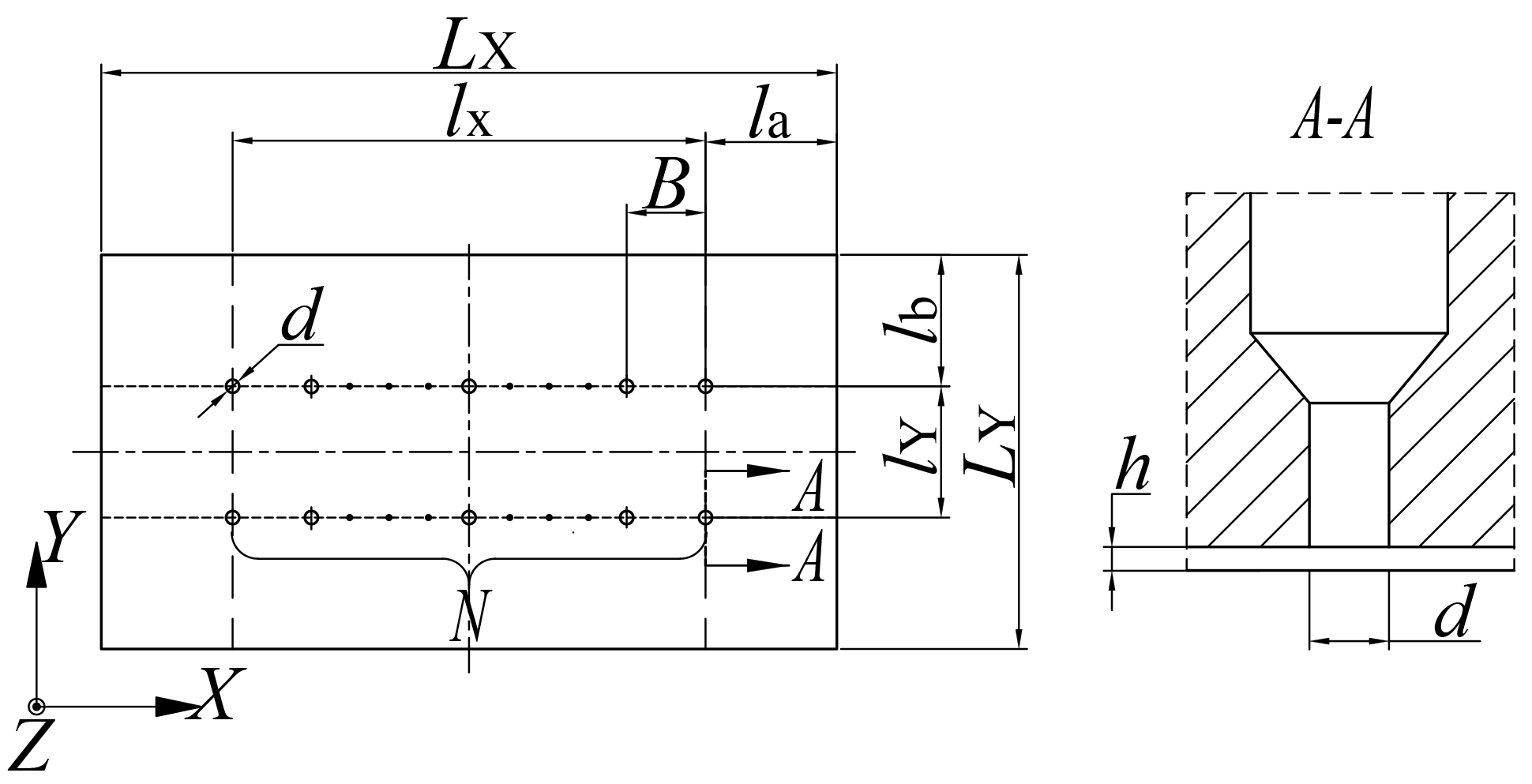
The rectangular aerostatic thrust bearing is illustrated in Figure 1. A Cartesian coordinate system is established, with the center of the bearing as the origin and the direction of the thickness of the film as the positive Z-axis. The dimensions of the bearing are LX in length and LY in width. The dimensions of the rectangular area enclosed by the orifice are lX and lY, respectively, and are located at the center of the bearing. The distance from the orifice to the edge of the bearing in the X and Y directions is designated as la and lb, respectively. The distance between each row of orifices is B, and the number of orifices is N. The diameter of the orifice is d. Calculate and analyze 12 different structures of rectangular bearings with dimensions of LX = 56 mm and LY = 30 mm. In this article, the studies were grouped according to the following parameters: N, la, lb, and d. The structural parameters and grouping details for all cases are listed in Table 1.
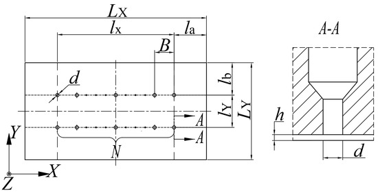
Figure 1.
Schematic diagram of rectangular aerostatic thrust bearing structure.

Table 1.
Bearing structure parameters and grouping.
2.2. Analytical Model
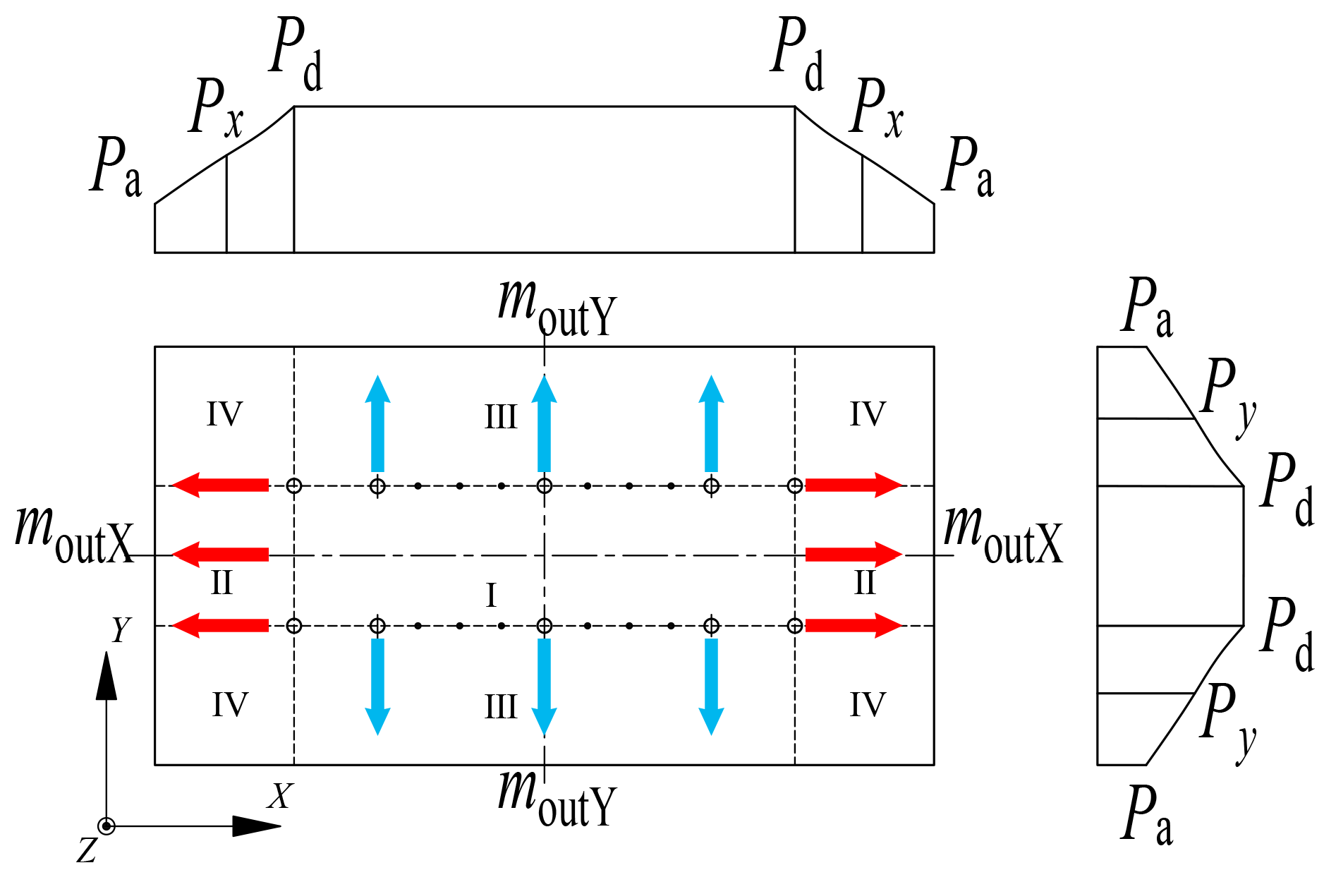
In order to facilitate the calculation of the two-dimensional fluid domain of rectangular aerostatic thrust bearings, we have adopted a partition calculation method based on the structural design and pressure distribution form of the bearings. As shown in Figure 2, the bearing surface is divided into two distinct zones: a gas supply zone and a dissipation zone. The gas supply zone is defined as the area surrounded by orifice (ASO), which is a rectangular zone centrally located within the bearing, while the dissipation zone is the area where high-pressure gas gradually flows out of the bearing. The dissipation zone is further divided into sub-zones II, III, and IV, while the gas supply zone is designated as sub-zone I.
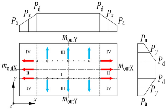
Figure 2.
Schematic diagram illustrating the partitioning, mass flow rate (red and blue arrows), and pressure distribution in the analytical modeling of a rectangular aerostatic bearing.
In accordance with the theory of gas lubrication, the linear gas source assumption is posited for discrete supply holes in order to facilitate the calculation of the analytical model. This implies that in the dissipation zone, both the X and Y directions are one-dimensional flows that are independent of one another. The pressure in the ASO is pressure Pd behind the orifice without attenuation. Moreover, due to the extremely small thickness of the film, it is commonly accepted that the pressure gradient in the direction of the film thickness is 0 and that the viscosity coefficient is constant. Consequently, the mass flow Expressions (1) and (2) for the X and Y directions of the bearing outlet can be derived from the fluid motion equation and mass continuity equation under steady-state conditions. The pressure in the equation represents the pressure distribution in regions II and III, and the pressure distribution Functions (3) and (4) in the corresponding regions can be obtained through integration. The flow within the film is isothermal.
Then, the bearing capacity of the aerostatic thrust bearing can be calculated as follows:
The stiffness of an aerostatic thrust bearing is defined as the derivative of the bearing capacity with respect to the thickness of the air film.
where the pressure Pd behind the orifice is unknown. By solving the continuity Equation (7) for the mass flow rate over the entire fluid domain, the pressure Pd can be obtained, as shown in Equation (8), detailed in Appendix A.
where Min represents the total inflow mass flow, MoutX = 2moutX and MoutY = 2moutY. The parameter ψ is contingent upon the flow state, with the sonic speed as the critical condition, as illustrated in Equation (9). Cd is the throttling coefficient, and according to the research in reference [26], this article takes it as 0.8.
However, due to the discrete distribution of orifices, it is inevitable that a certain pressure drop will occur between the orifices. The utilization of the pressure Pd behind the orifice for the representation of the uniform pressure of the ASO will result in an overestimation of the analytical calculation’s bearing capacity. It is necessary to employ an average pressure (PdAVE) in lieu of Pd. An examination of the analytical model reveals that the PdAVE is predominantly contingent upon the geometric parameters of the ASO of the bearing. Consequently, this article has investigated the influence of four parameters, N, la, lb, and d, on the PdAVE under three distinct supply pressures, namely 0.4 MPa, 0.5 MPa, and 0.6 MPa.
2.3. Numerical Model
2.3.1. Meshing
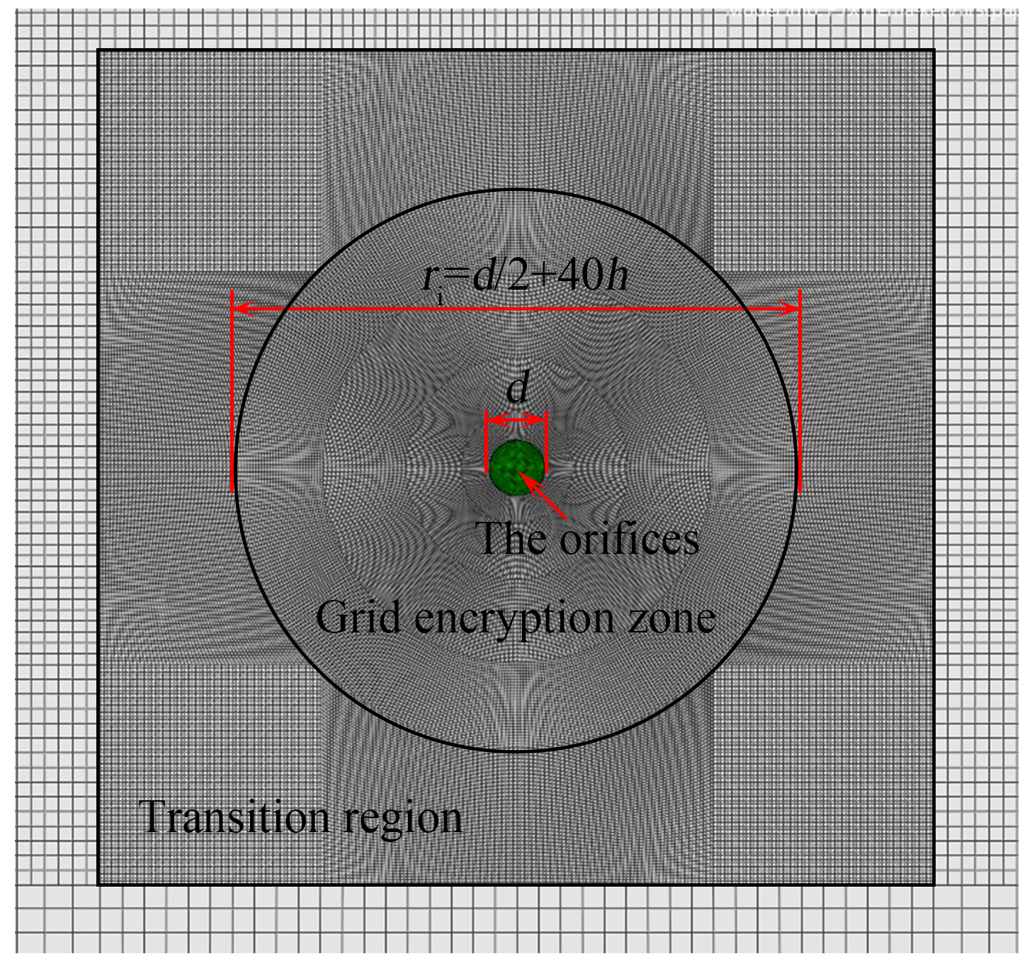
The working surface of the rectangular bearing is a symmetrical structure, and a volume finite element model can be established by taking one quarter of it for calculation. In numerical calculations, due to the significant difference between the gas film and the size of the bearing structure, if the size and quality of the mesh partition is determined solely based on the thickness of the gas film, it will greatly increase the number of meshes and greatly reduce the computational efficiency. Therefore, this article adopts the form of local refinement to divide the mesh. We combined the analysis of the flow field inside the gas film behind the orifice in reference [27] with the empirical Formula (10) for the full development radius of the viscous resistance obtained by experiments in reference [11] to determine the mesh refinement region, as shown in Figure 3. Use interfaces to connect meshes of different sizes.
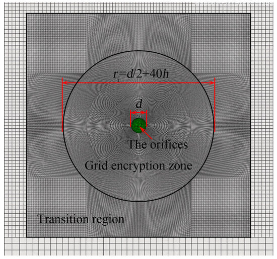
Figure 3.
Mesh refinement area and refined mesh. (The red lines and arrows demarcate the different ranges of mesh refinement).
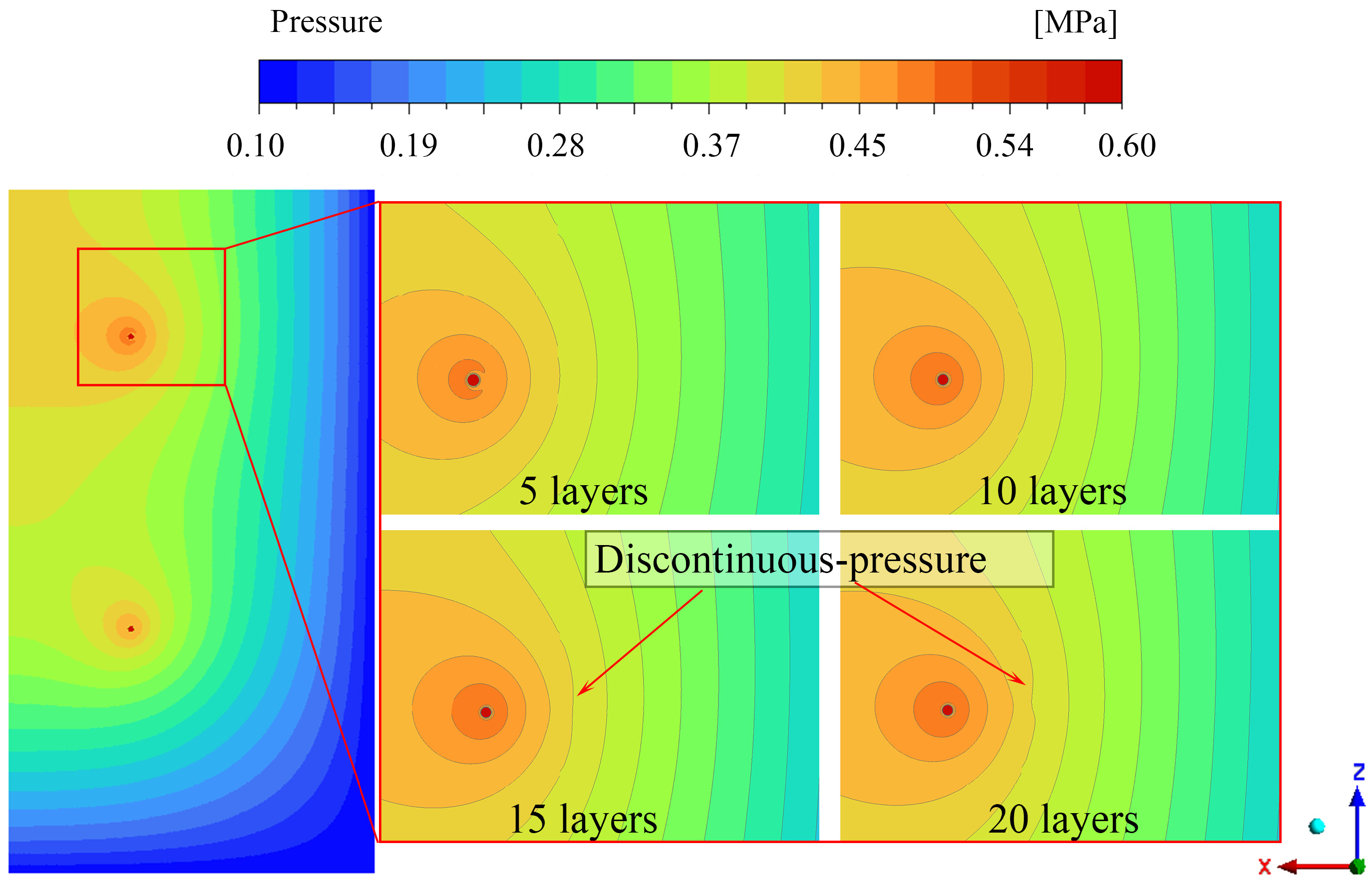
In addition to the refinement of the local mesh, the mesh layering of the air film gap also determines the quality of the mesh and the accuracy of the simulation calculations. In order to determine the appropriate number of mesh layers for the air film gap, taking a 10 μm air film thickness as an example, the air film gap was divided into 5, 10, 15, and 20 mesh layers according to mesh sizes of 2 μm, 1 μm, 0.67 μm, and 0.5 μm, respectively, for the comparison. We compared the bearing capacity of aerostatic bearings under different stratification conditions at absolute supply pressures of 0.4 MPa, 0.5 MPa and 0.6 MPa, as well as the pressure cloud map at a supply pressure of 0.6 MPa. The comparison of bearing capacity is shown in Table 2, and the pressure cloud map is shown in Figure 4.
Table 2.
Comparison of bearing capacity.
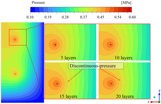
Figure 4.
Pressure distribution under different layers of gas film gap at P0 = 0.6 MPa.
From the bearing capacity in Table 2, it can be seen that when the number of layers is ≥10, the bearing capacity tends to a constant value with fluctuations not exceeding ±1%. Moreover, it can be seen from Figure 4 that when the number of layers is divided into 15 and 20 layers, there are obvious pressure defects at the edge of the mesh transition zone. Overall, in order to ensure the accuracy of the simulation calculations, it is optimal to divide the air film gap into 10 layers, with a single-layer grid thickness of 1 μm.
2.3.2. Numerical Methods and Control Equations
The gas flow in an aerostatic bearing is a three-dimensional, steady-state, compressible high-speed gas flow problem between flat plates. A large number of scholars have found [27,28,29] that when the thickness of the film is large, supersonic phenomena exist in the area where the orifice intersects the film. Moreover, according to the Reynolds number calculation formula Re = ρvd/μ, it can be calculated that the Reynolds number at the interface between the orifice and the film exceeds 2800, indicating that the flow here is turbulent. Therefore, in this paper, the Realizable k-ε turbulence model is used for the calculation. To ensure the accuracy of the Realizable k-ε turbulence model at low Reynolds numbers, the Enhanced Wall Treatment (EWT) was used. In addition, a mesh adaptation method was used in the calculation to ensure that the near-wall mesh met the EWT requirement for the first mesh height, i.e., y + < 5.
In the Cartesian coordinate system, the continuity equation, the motion equation, and the energy equation for three-dimensional, steady-state, and compressible flow can be written in the following form, according to the general form of the control equations in computational fluid dynamics:
where δij is the Kronecker function. Fluid is an ideal gas. The molecular viscosity μ of the gas is given by Sutherland’s law. And the turbulent viscosity μt is a function of the turbulent kinetic energy k and the turbulent dissipation rate ε, given by Equation (14).
The control equation composed of the above three equations contains two additional unknowns, k and ε. Therefore, it is necessary to supplement the transport equations of both under steady-state conditions to achieve closure of the system of equations.
where ac is the sonic speed and S is the modulus of the average stress tensor.
In simulation calculations, the pressure–velocity coupling calculation uses the SIMPLE algorithm, and the second-order upwind scheme is used to interpolate and solve the control equations. When the import and export flow rates tend to be equal and the residuals of various velocities, energies, k, ε, and continuity equations are less than 10−5 and tend to be stable, the calculation is considered to have converged and is stopped.
2.4. Experimental Setup
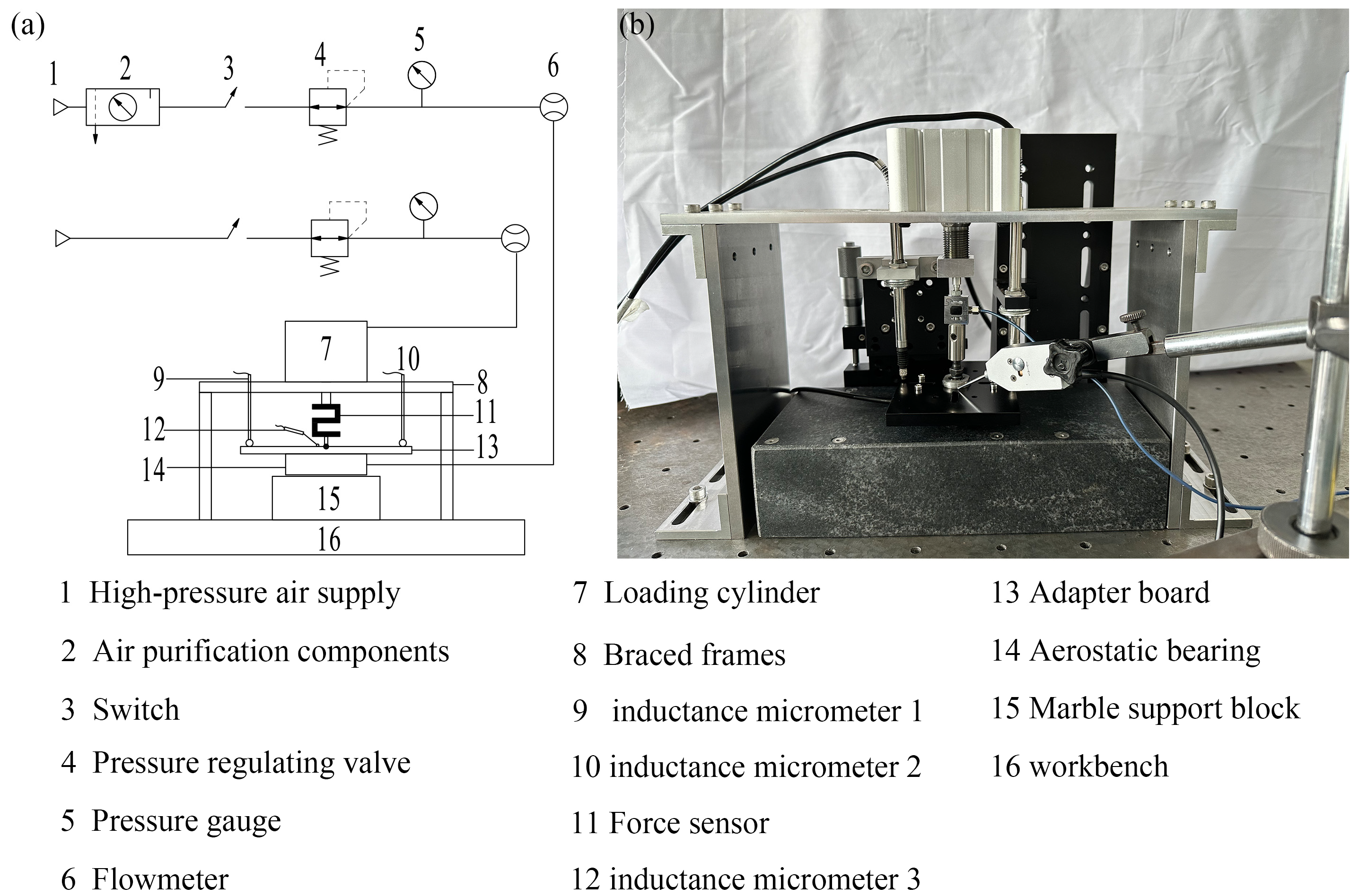
In order to verify the accuracy and effectiveness of the simulation results and the proposed method for calculating the average pressure in the ASO, an aerostatic bearing test platform was built as shown in Figure 5b, and its principle is shown in Figure 5a. The load is applied through a cylinder and the balance force between the bearing and the cylinder is tested as the bearing capacity using a force sensor. The thickness of the film is measured with inductance micrometers. To ensure the accuracy of the film thickness, three different points are measured simultaneously using three inductance micrometers, ensuring that the entire measurement plane only moves up and down. The minimum resolution of the three inductance micrometers is 0.1 μm.
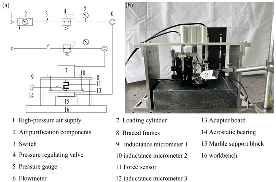
Figure 5.
Experimental design. (a) experimental principle and (b) experimental setup.
3. Results
The simulation is conducted under the following boundary conditions: pressure inlet, pressure outlet, and isothermal wall. The absolute supply pressures at the pressure inlet are 0.4 MPa, 0.5 MPa, and 0.6 MPa, respectively, while the pressure at the pressure outlet is 0.1 MPa, equivalent to the ambient pressure.
3.1. The Difference Between the Average Pressure PdAVE and the Pressure Pd Behind the Orifice
In numerical simulations, the area-weighted average method may be employed to calculate the average value of the pressure field in the ASO, thereby obtaining the average pressure, PdAVE, in the ASO.
In this study, the type 2 bearing structure is employed as a reference for research. When the thickness of the film is 10 μm, the average pressure of the bearing is shown in Table 3.
Table 3.
Average pressure of type 2 bearing at a film thickness of 10 μm.
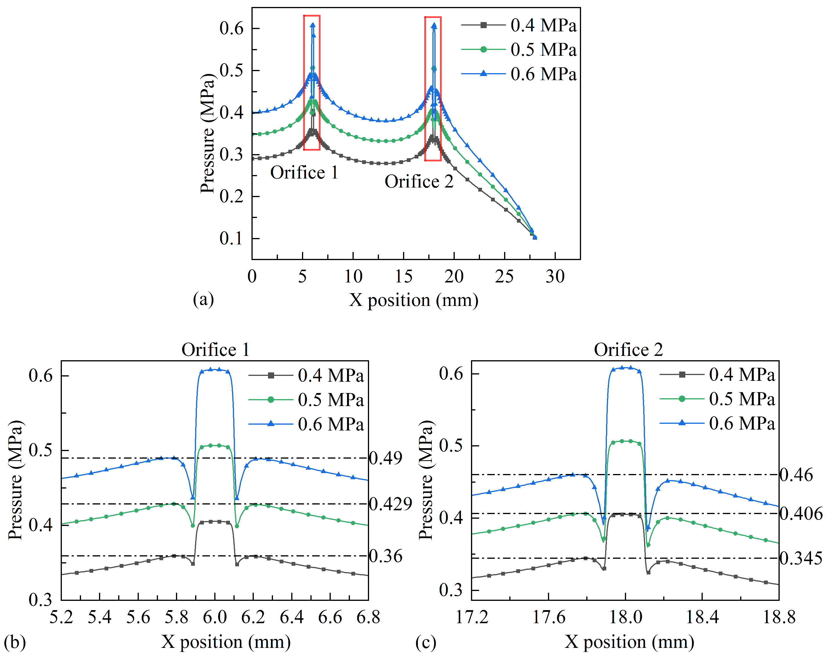
The pressure behind the orifice in the same situation can be obtained by analyzing the pressure drop phenomenon and the value of the pressure behind the orifice, as outlined in reference [11]. By taking the cross-section of the rectangular bearing passing through the center of the orifice in the X-direction and employing the calculation principle of the bearing capacity, it is possible to draw a curve representing the pressure projection values of the X-direction cross-section on the bearing plane, as shown in Figure 6. This curve is the pressure distribution curve passing through the center section of the orifice.
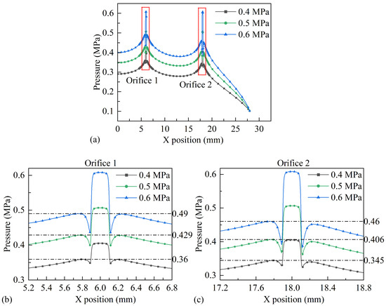
Figure 6.
The pressure distribution at the center section of the X-direction orifice of the type 2 bearing. (a) The pressure distribution of the one quarter model; (b) enlarged image of orifice 1; (c) enlarged image of orifice 2.
The research of numerous researchers [11,27] on the pressure drop phenomenon after the orifice and the rapid recovery phenomenon after the pressure decreases indicates that the maximum point after the pressure recovery is the pressure Pd behind the orifice. Figure 6 illustrates that the pressure is at its maximum at orifice 1 in proximity to the symmetry plane, subsequently declining as it approaches the edge of the bearing. The pressure at orifice 2 is slightly lower than that at orifice 1 due to the presence of pressure superposition at the center of the bearing. At the edge, the superposition effect on the pressure behind the orifice is absent, resulting in a pressure value that is in close alignment with the calculated theoretical value. Consequently, the pressure value indicated in Figure 6c represents the pressure Pd behind the orifice. From Figure 6, it can be seen that the pressure behind the orifice quickly reaches a peak, while there is a significant decrease in pressure between the orifices. Consequently, utilizing the pressure Pd behind the orifice in the analytical model to ascertain the bearing capacity of the ASO results in an overestimation of the bearing capacity and stiffness of the aerostatic bearing, which in turn leads to an erroneous design of the aerostatic bearing.
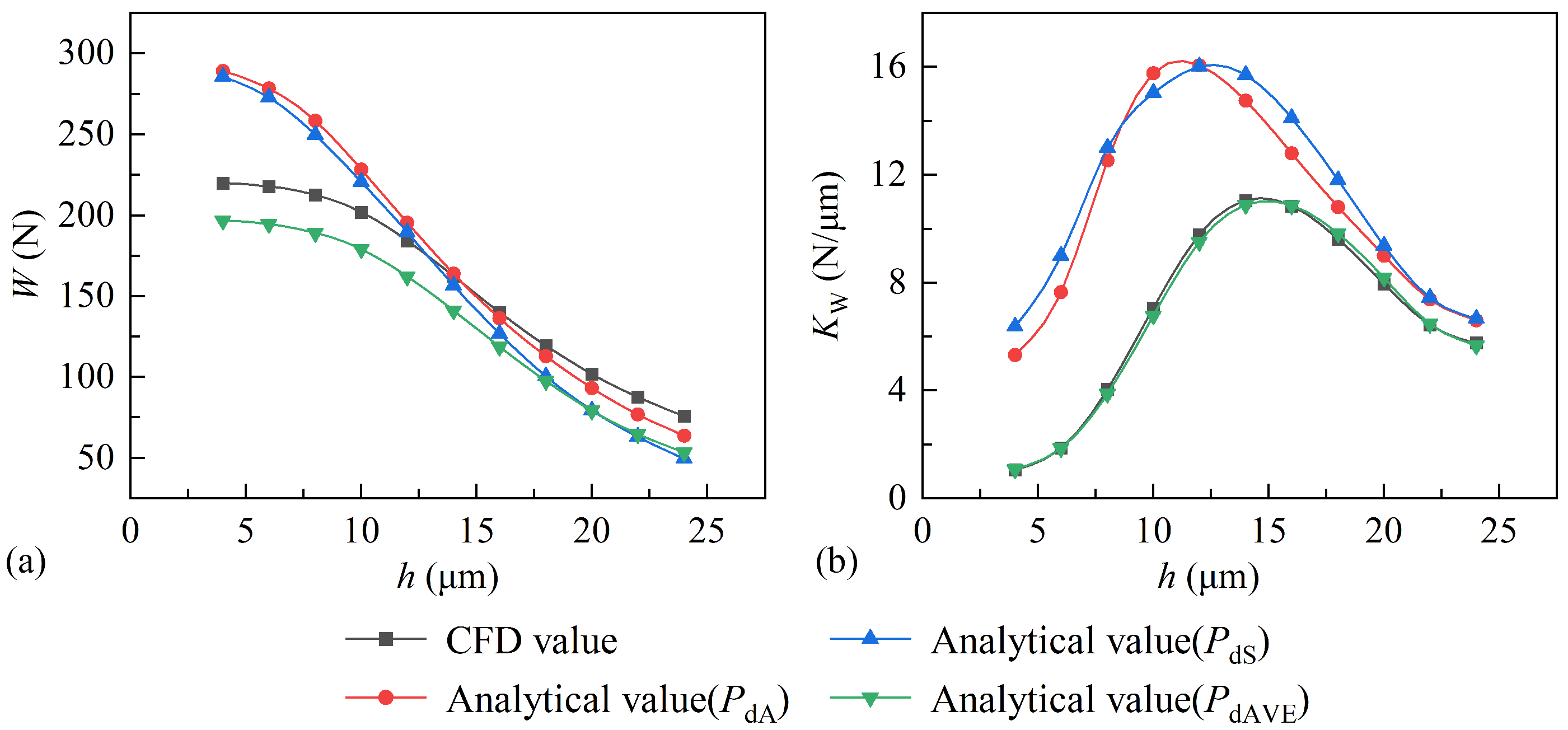
The pressure behind the orifice, calculated using Equation (8), is PdA. The pressure behind the orifice, obtained from the simulation results in Figure 6c, is PdS. The average pressure in the ASO is PdAVE. The bearing capacity and stiffness curves of the aerostatic bearing are to be calculated by applying three different pressures into the analytical Equations (5) and (6), as shown in Figure 7.
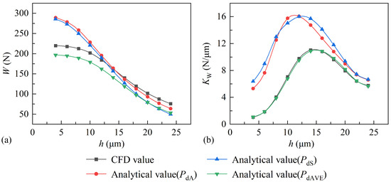
Figure 7.
Comparison between (a) bearing capacity and (b) stiffness calculated under different pressures and simulation results.
Figure 7 illustrates that the bearing capacity and stiffness values calculated using PdA and PdS are nearly identical, yet they diverge significantly from the results obtained through CFD, both of which overestimate the bearing capacity and stiffness of the aerostatic bearing. The calculated bearing capacity based on PdAVE is lower than the simulation results. However, there is a high degree of overlap in the stiffness values between the two. The analytical calculation results obtained from this are more in line with the safe and accurate design concept of aerostatic bearings.
3.2. Influence of Structural Parameters and Supply Pressure on Average Pressure
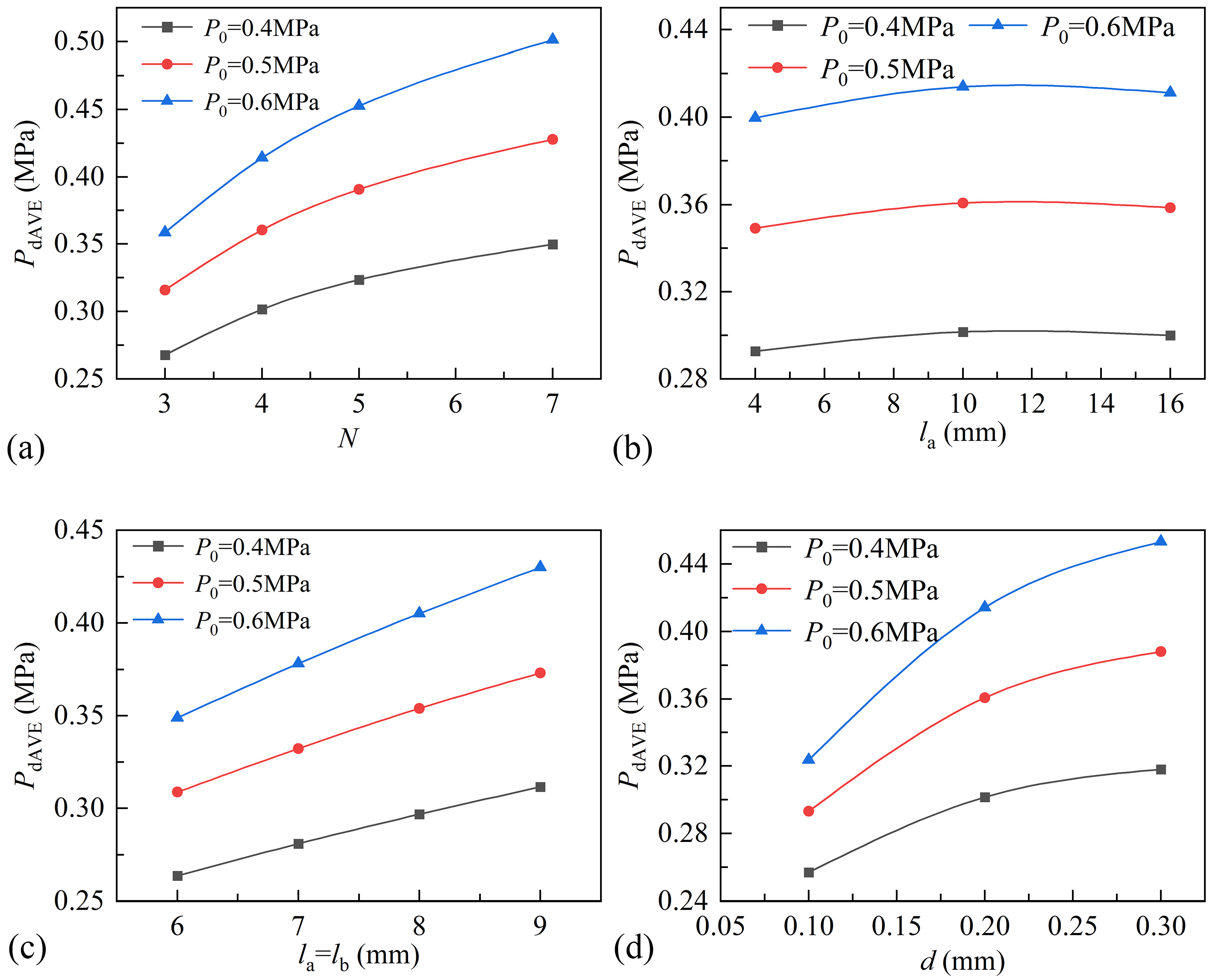
From the establishment of the analytical model, it can be seen that the main influencing parameters for the design of rectangular aerostatic thrust bearings include the number of orifices, the distance from the orifices to the edge of the bearing, and the diameter of the orifices. Accordingly, this paper employs CFD simulation to investigate four distinct variable designs: the number of orifices in a single row, the distance from the orifices in the X-direction to the edge, the equal distance from the orifices in the X and Y directions to the edge, and the diameter of the orifices. The impact of these four parameters on the average pressure within the ASO at a film thickness of 10 μm is illustrated in Figure 8.
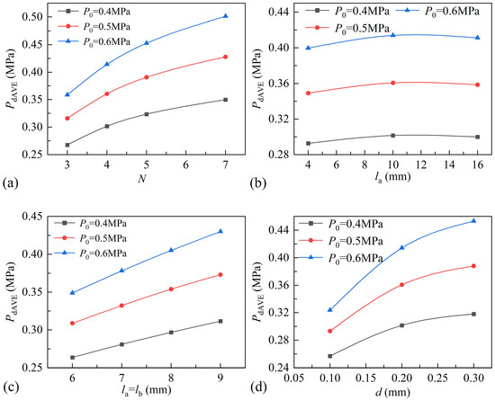
Figure 8.
The influence of four parameters on the average pressure (PdAVE) in the ASO. The four parameters are (a) the number of single row orifices N, (b) the distance from the orifice to the edge in the X-direction la, (c) the distance from the orifice with equal upward changes in X and Y directions to the edge (la = lb), and (d) the diameter of the orifice d.
Figure 8 illustrates that the relationship between the average pressure PdAVE in the ASO and various structural parameters shows an increasing trend, and the slope gradually decreases. As can be seen from Figure 8b, when only la is varied, the change in PdAVE is very small. However, from Figure 8c, it is evident that when la = lb is maintained and the distance from the orifices to the bearing edge is increased simultaneously, PdAVE shows a significant increase. This indicates that, for the same number of orifices, a smaller supply area leads to a more concentrated high-pressure region, resulting in a larger PdAVE. However, when la is increased alone, the number of orifices is also altered. Combining this with Figure 8a, it can be observed that when the number of orifices decreases, PdAVE decreases accordingly. Therefore, in Figure 8b, the variation in PdAVE is neutralized due to the combined influence of the two structural parameters. Furthermore, the graph illustrates that the higher the supply pressure, the higher the average pressure. The average pressure curves under different supply pressures exhibited a near-parallel relationship. The average pressure curve under a supply pressure of 0.6 MPa displays distinctive variations solely in the number and diameter of orifices. This variation indicates that when the throttling area is relatively small, increasing the supply pressure has a limited effect on enhancing the load-carrying capacity and stiffness of the bearing. The primary reason is that a smaller throttling area imposes a greater restriction on the mass flow rate. Under such conditions, the influence of the mass flow rate on the pressure downstream of the throttling orifice becomes more pronounced, while the supply pressure fails to exert its intended impact effectively.
The aforementioned four parameters are capable of corresponding to the geometric parameters present within the analytical Expression (8). The performance of la and lb in the expression is the ratio of the side length corresponding to the ASO, which is a dimensionless geometric parameter. The influence of the four parameters on the average pressure PdAVE can be unified as the influence of the geometric parameter term in Expression (8). As shown in Equation (18), normalizing d and h and obtaining function f for N, d, la, lb, and h.
where d0 = 0.2 mm, h0 = 10 μm.
As shown in Equation (19), the average pressure within the gas supply region is expressed as a dimensionless quantity, defined as the average pressure coefficient.
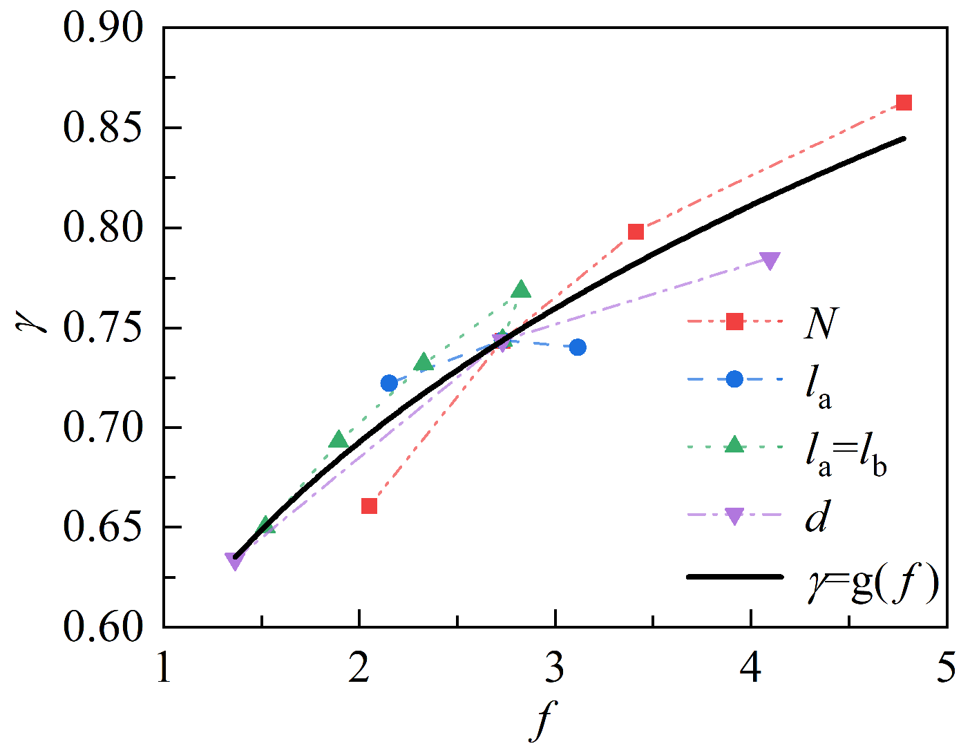
Figure 9 illustrates the relationship between the dimensionless structural parameters and the average pressure coefficient under a gas film thickness of 10 μm and a gas supply pressure of 0.4 MPa. As can be observed in the figure, the relationship between the average pressure coefficient and the dimensionless structural parameters is consistent with the relationship between the average pressure and each structural parameter, as illustrated in Figure 8. Therefore, it is reasonable to unify the four structural parameters using Expression (18).
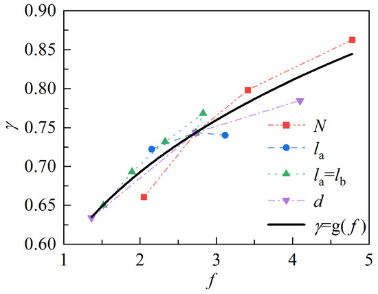
Figure 9.
The relationship between the average pressure coefficient γ and the uniform dimensionless structural parameter f when h = 10 μm and P0 = 0.4 MPa.
Furthermore, as can be observed from Figure 9, among the four structural parameters, the number of orifices N and the diameter of the orifices d exhibit the most significant influence on the average pressure coefficient. In contrast, the influence of la and lb is primarily concentrated in the range where the average pressure coefficient is less than 0.78, indicating that the average pressure is predominantly affected by the number of orifices N and the diameter of the orifices d. However, the trends of the individual variations in the four structural parameters on the average pressure coefficient are approximately consistent. Therefore, an approximate function about f can be used to describe the relationship between different structural parameters and the average pressure coefficient. This approximate function is a power function, as shown in Equation (20), and the approximate curve it depicts is γ = g (f) in Figure 9.
From Expression (8), it can be observed that the pressure behind the orifice is not only affected by the four structural parameters mentioned above, but also by the thickness of the gas film. Consequently, Expression (20) can only represent the average pressure coefficient when the thickness of the gas film is 10 μm. When the thickness of the gas film is different, the relationship between the average pressure coefficient γ and the dimensionless structural parameter f is still approximately in the form of a power function, but the exponent and coefficient of the power function will vary with the thickness of the gas film. The approximate function curve between the average pressure coefficient γ and the dimensionless structural parameter f under different film thicknesses is shown in Figure 10.
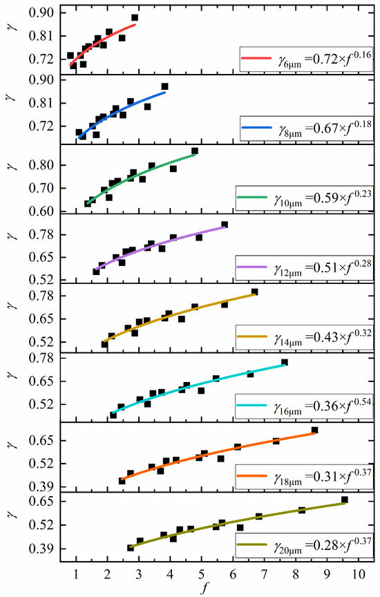
Figure 10.
The approximate function curve between the average pressure coefficient γ and the dimensionless structural parameter f under different film thicknesses.
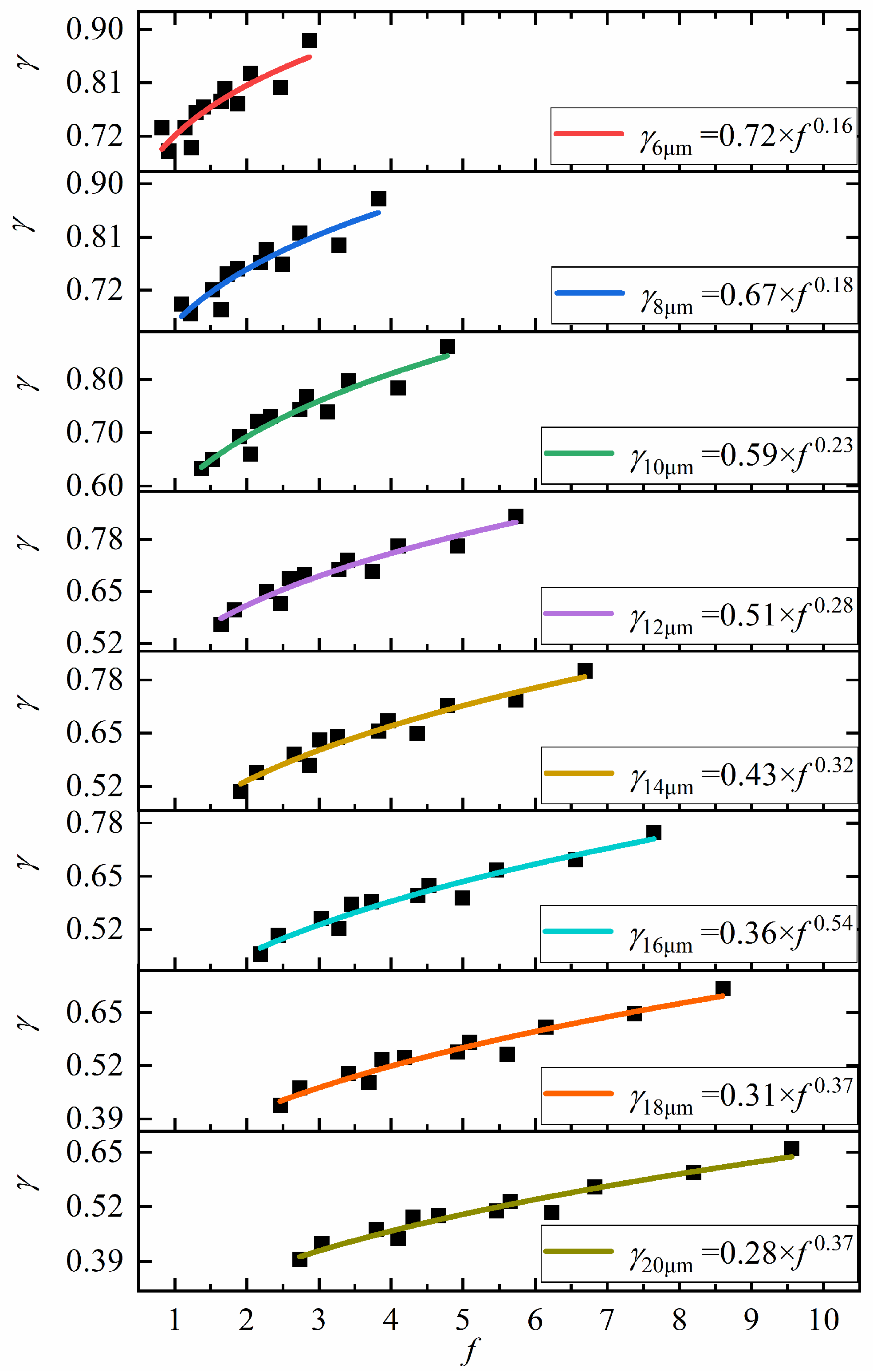
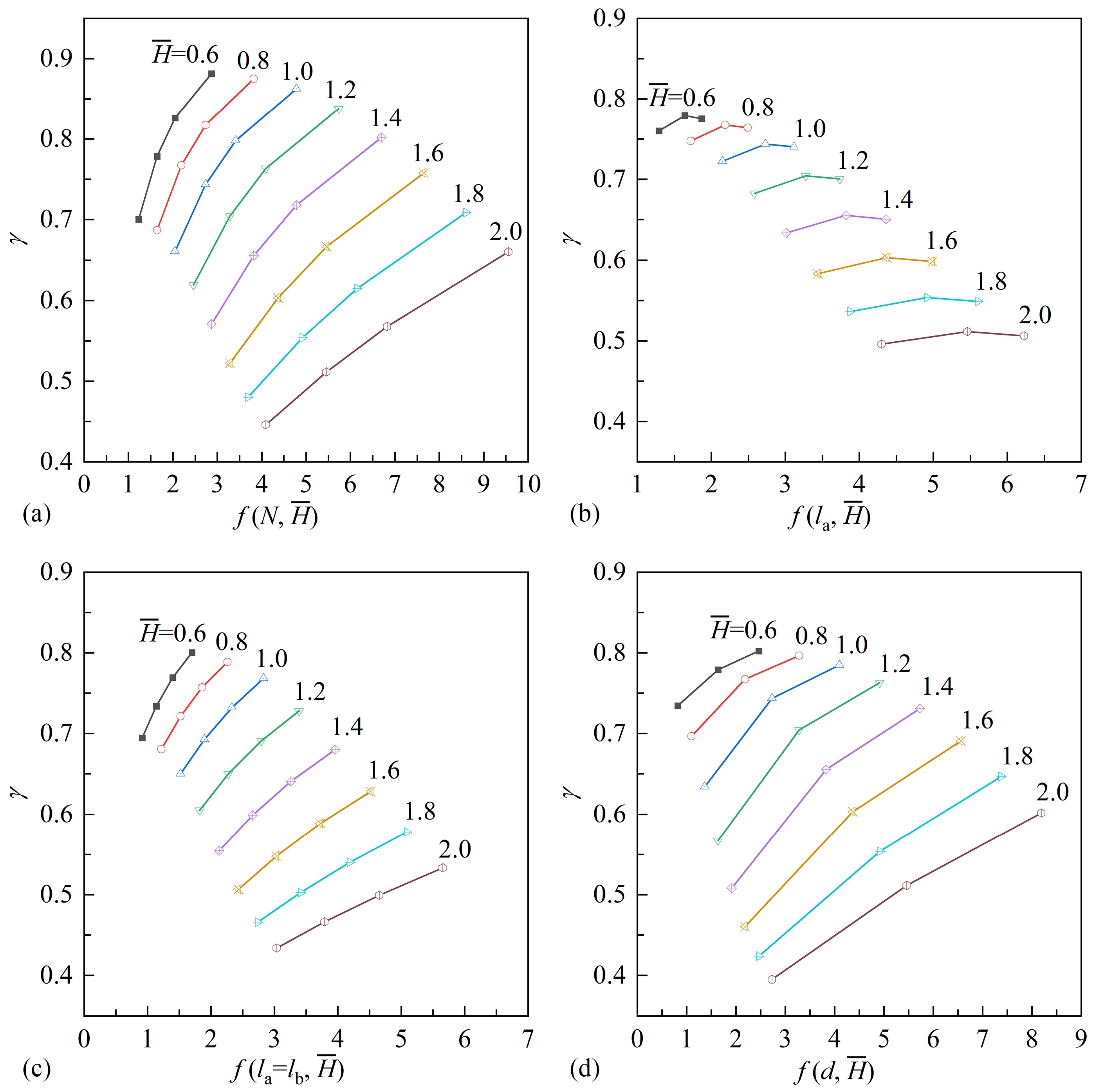
In order to extend the relationship between the average pressure coefficient γ and the dimensionless structural parameter f to all ranges of film thickness, it is necessary to provide the exponent and coefficient of the power function with respect to the variation in film thickness. The relationship between the average pressure coefficient γ and the dimensionless structural parameter f for various structural parameters at different film thicknesses is shown in Figure 11.
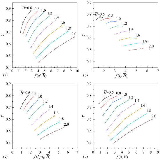
Figure 11.
Under different film thicknesses, the influence of the structural parameter: (a) the number of single row orifices N; (b) the distance from the orifice to the edge in the X-direction la; (c) the distance from the orifice with equal upward changes in X and Y directions to the edge (la = lb); and (d) the diameter of the orifice d on the average pressure coefficient γ.
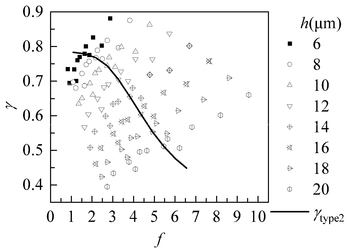
Figure 11 illustrates that in any structural design, the trend of the relationship between the average pressure coefficient γ and the dimensionless structural parameter f is very similar when changing the thickness of the gas film. As the thickness of the gas film increases, the average pressure coefficient first slowly decreases, then the proportion of decrease gradually increases, and finally the proportion of decrease gradually decreases again. As shown in Figure 12, by summarizing all the data and selecting a structural design (such as type 2), the average pressure coefficient point at this time is connected by a curve. It can be observed that this trend is similar to the bearing capacity curve of the hydrostatic bearing. Consequently, the coefficients and exponents in the approximate function between γ and f are a cubic function related to film thickness h. This function is presented in Expression (21).

Figure 12.
The relationship between the average pressure coefficient γ and the dimensionless structural parameter f in the design of fixed structural parameters.
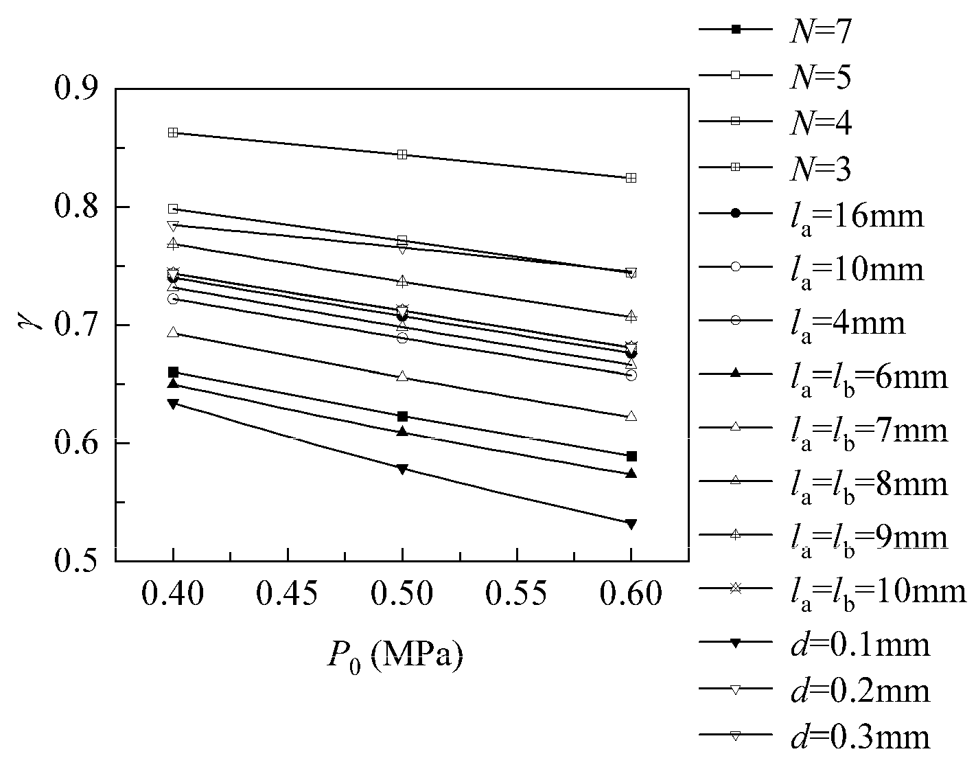
Figure 13 illustrates the relationship between the average pressure coefficient γ and the supply pressure P0 for a gas film thickness of 10 μm across different structural designs, calculated at supply pressures of 0.4 MPa, 0.5 MPa, and 0.6 MPa. From the figure, it can be observed that in all structural design cases, the variation in γ with P0 is monotonically decreasing. Furthermore, the variation curves under different structural conditions are approximately parallel. Therefore, based on the aforementioned study of a supply pressure of 0.4 MPa, it can be posited that there is a fixed scaling factor, defined as Γ, between different supply pressures. This factor is the slope of the curve in Figure 13. It is possible to summarize the two slopes of all curves in Figure 13 and plot them as a vertical line graph (Figure 14) in order to analyze the effects of structural parameters and changes in supply pressure on Γ.
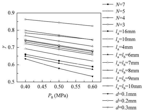
Figure 13.
The relationship between the average pressure coefficient γ and the supply pressure P0 when the film thickness is 10 μm.
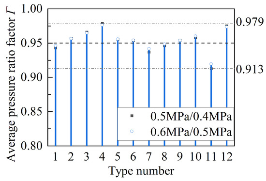
Figure 14.
The influence of structural parameters on the scaling factor Γ.
It can be calculated that the mean value of the scaling factor Γ for all 12 structural forms is 0.95. Accordingly, the analysis of changes in the scaling factor Γ will be conducted using 0.95 as a reference value. Figure 14 illustrates that the maximum value of the scaling factor Γ is 0.979 and the minimum value is 0.913 across all structural designs. In comparison to the value of 0.95, the discrepancy is less than 4%. This suggests that alterations in structural parameters have a limited influence on the scaling factor Γ and can be disregarded. Furthermore, the scaling factor Γ between different supply pressure ratios exhibits a high degree of overlap. In conclusion, when the supply pressure is increased in accordance with an atmospheric pressure value, a uniform scaling factor can be employed for calculations.
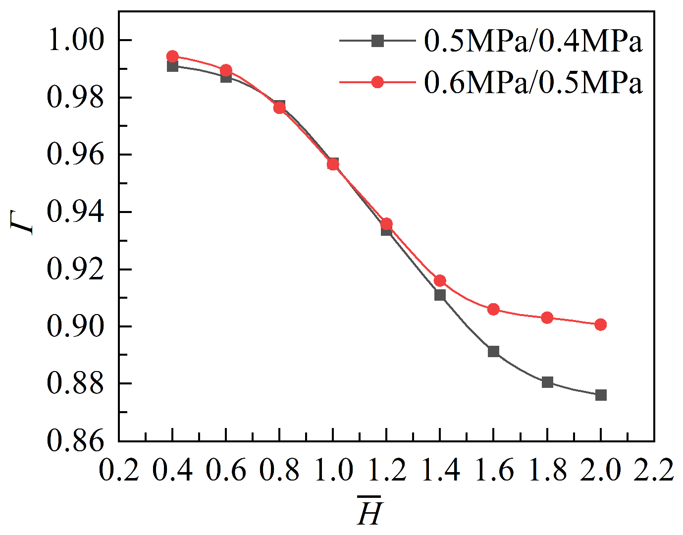
Using the structural design of type 2 as a reference, plot the relationship between the scaling factor Γ and the dimensionless film thickness in Figure 15. From the graph, it can be observed that the scaling factors between the supply pressure of 0.4 MPa and 0.5 MPa, and between 0.5 MPa and 0.6 MPa, exhibit a high degree of coincidence when the gas film thickness is less than 14 μm. When the film thickness is greater than 14 μm, the difference between the two gradually increases and tends to a fixed value, with a difference of approximately 0.025. In comparison to the mean of the two, the error is not more than 3%. Therefore, this scaling factor can be written as a unified approximation function about the dimensionless film thickness, as shown in Equation (22).

Figure 15.
The relationship between the scaling factor Γ and the dimensionless film thickness.
Ultimately, by combining Equations (21) and (22), the complete expression for calculating the average pressure coefficient, Equation (23), can be derived as follows:
Equation (23) is primarily designed for the static performance calculation of rectangular aerostatic thrust bearings with double exhaust orifices. Initially, Equation (23) is utilized to estimate the average pressure within the ASO of the bearing. By substituting the average pressure for the pressure downstream of the orifice, the load capacity and stiffness characteristics of the aerostatic thrust bearing can be accurately and effectively estimated.
3.3. Comparison and Verification Between Experiments and CFD Simulations
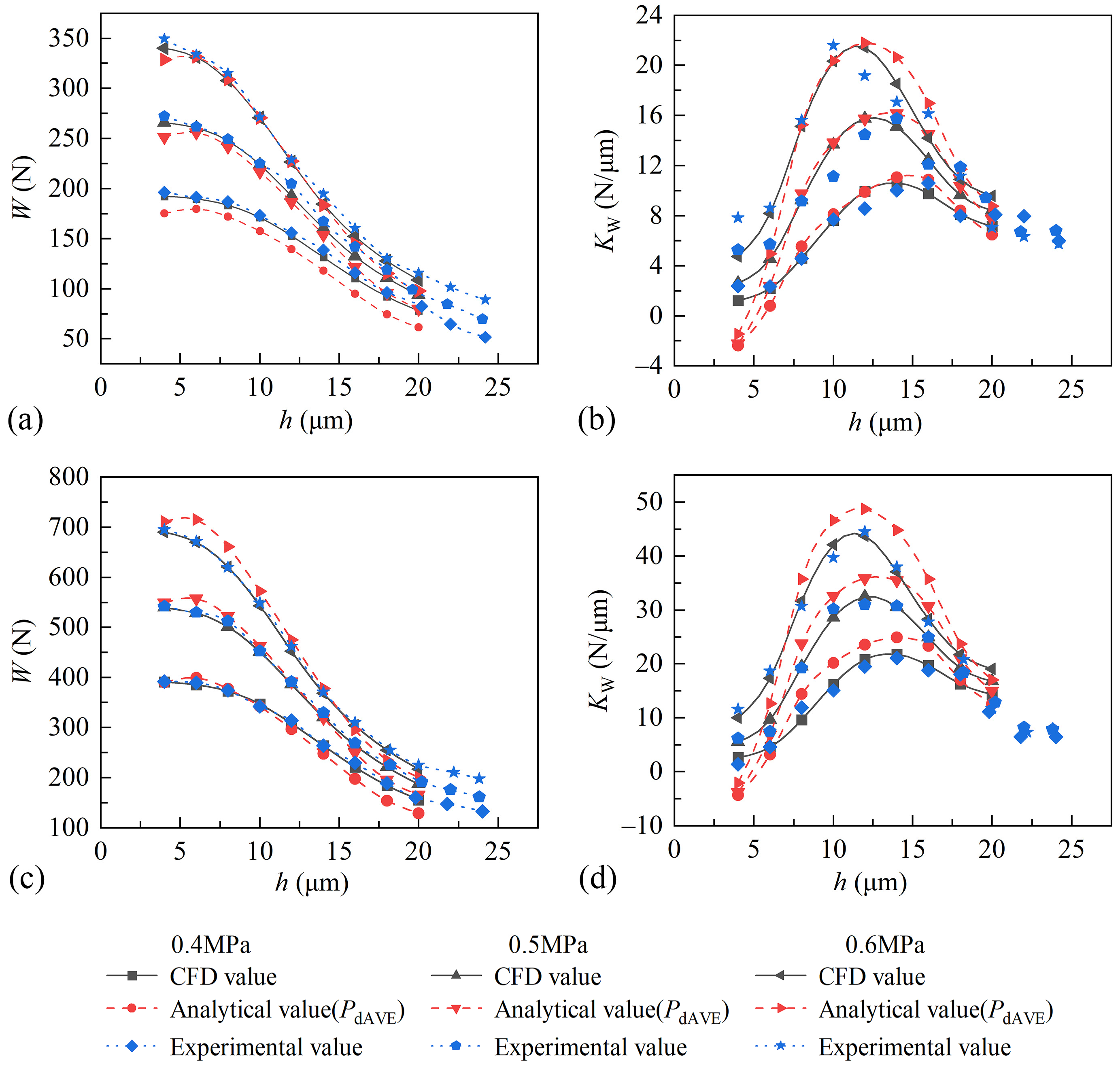
From the 12 types of bearing structures studied, type 1 was selected as the experimental object. Experiments were conducted at supply pressures of 0.4 MPa, 0.5 MPa, and 0.6 MPa. A comparison of the bearing capacity and stiffness obtained from simulation, analytical calculations, and experiments is presented in Figure 16a, b, respectively. In order to verify the effectiveness and accuracy of the analytical method more widely, a new bearing structure, designated as type 13, was introduced, with a structural parameter of LX = 80 mm, LY = 40 mm, lX = 60 mm, lY = 20 mm, la = 10 mm, lb = 10 mm, B = 20 mm, N = 4, and d = 0.2 mm. It is necessary to conduct identical experiments and comparisons, as shown in Figure 16c,d.
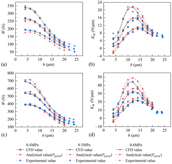
Figure 16.
Comparison of static characteristics of bearings obtained from CFD simulation, analytical models, and experiments. (a) Bearing capacity of type 1; (b) stiffness of type 1; (c) bearing capacity of type 13; (d) stiffness of type 13.
Figure 16 illustrates that the experimental values are largely aligned with the CFD values. The discrepancy in stiffness can be attributed to the stability of the experiment. In the experiment, the loading adjustment of the cylinder necessitates a specific time to achieve equilibrium with the gas film. Consequently, fluctuations in the measured bearing capacity result in corresponding fluctuations in the stiffness curve. However, the trend of the curve observed in the experiment is entirely consistent with the simulation. Furthermore, the stiffness comparison chart reveals that the optimal stiffness values for both designs fall within the range of 8–16 μm for the air film thickness, which is the optimal working range for the bearing.
As illustrated in Figure 16a, c, the bearing capacity results for type 1 exhibit a notable discrepancy under a gas supply pressure of 0.4 MPa. This finding aligns with the observations documented in Figure 7. In the design of type 13, the difference between the calculated results of the analytical method and other results is primarily in the case of a gas film smaller than 8 μm. In the optimal working range, the analytical values exhibit a notable deviation, with an error of 10.6% compared to the CFD values and an error of 14% compared to the experimental values, occurring solely under a supply pressure of 0.4 MPa and a gas film of 16 μm. In other instances, the difference is within 5%.
As illustrated in Figure 16b,d, the thickness of the gas film corresponding to the maximum stiffness exhibits a gradual decrease under different supply pressures. However, the range of optimal stiffness remains consistent. In type 1, there is a discernible discrepancy between the maximum stiffness point of the experimental value and the CFD and analytical values, fluctuating within a range of ±2 μm. In type 13, the analytical value is relatively larger than the CFD value and experimental value. At a supply pressure of 0.4 MPa, there is a discrepancy of 20% between the analytical and experimental values for the maximum stiffness. However, in all cases, the gas film thickness corresponding to the maximum stiffness value is found to be consistent.
In conclusion, the analytical calculation method proposed in this article is highly accurate in predicting bearing capacity. However, different designs exhibit varying degrees of discrepancy in the prediction of stiffness. Nevertheless, the optimal stiffness working range of the aerostatic bearing can still be accurately estimated, thereby providing precise and effective guidance for the design of aerostatic bearings.
4. Conclusions
By examining the impact of disparate structural parameters of aerostatic bearings on the average pressure within the ASO, an analytical model was proposed for calculating the static character of aerostatic bearings using the average pressure in the ASO. Ultimately, the accuracy and efficacy of the analytical model were validated through experiment. The research results are as follows:
(1) By using the average pressure in the ASO instead of the pressure behind the orifice for analytical calculation, the predicted static characteristics of the bearing are more accurate and secure.
(2) Among the four structural parameters (N, la, lb, and d), the number and diameter of the orifices that determine the throttling area exert a greater influence on the average pressure.
(3) The four parameters correspond to the structural terms in the bearing capacity analysis model, and the dimensionless structural terms are employed to unify the influence of the four parameters on the average pressure in the ASO. In combination with the influence of the gas film thickness, an approximate expression for calculating the average pressure coefficient is provided.
(4) The impact of changes in gas supply pressure on average pressure is approximately linear, and a unified scaling factor expression is provided for different changes in supply pressure.
(5) The simulation method employed in the article was validated through experiment, and the approximate expression of the average pressure in the ASO is also effective and accurate in predicting the static characteristics of the aerostatic bearing.
Author Contributions
Conceptualization, J.W. (Jianwei Wu) and J.Z.; methodology, J.Z. and J.W. (Jianwei Wu); software, J.Z. and J.W. (Jiyao Wang); validation, J.Z. and H.L.; formal analysis, J.W. (Jianwei Wu) and H.L.; investigation, J.Z.; resources, J.W. (Jianwei Wu) and P.Z.; data curation, J.Z. and J.W. (Jiyao Wang); writing—original draft preparation, J.Z.; writing—review and editing, J.Z. and H.L.; project administration, J.W. (Jianwei Wu) and P.Z.; funding acquisition, J.W. (Jianwei Wu) and P.Z. All authors have read and agreed to the published version of the manuscript.
Funding
This research was funded by the National Natural Science Foundation of China, grant number 52175499 and 52105547, and the Natural Science Foundation of Heilongjiang Province, grant number LBH-Z21063.
Data Availability Statement
Data are contained within the article.
Acknowledgments
The authors would like to thank all the reviewers who participated in the review of this manuscript.
Conflicts of Interest
The authors declare no conflicts of interest.
Abbreviations and Nomenclature
The following abbreviations are used in this manuscript:
| Abbreviations | |||
| CFD | computational fluid dynamics | ||
| EWT | enhanced wall treatment | ||
| ASO | area surrounded by orifice | ||
| Nomenclature | |||
| h | gas film thickness | μ | air viscosity |
| P0 | gas supply pressure | R | gas constant, 287 J/(kg K) |
| Pa | standard atmospheric pressure | T | absolute temperature, 293 K |
| ρ | density | κ | gas specific heat ratio, 1.4 |
| A | single throttling area | λ | thermal conductivity |
| Cd | discharge constant | f | dimensionless geometric parameter |
| PdAVE | average pressure in the ASO | γ | PdAVE/P0, the average pressure coefficient |
| Asup | the area surrounded by orifice | Γ | scaling factor of gas supply pressure |
| Ai | single grid area | W | bearing capacity |
| Pd | orifice downstream pressure | KW | bearing stiffness |
Appendix A
Based on the assumptions regarding the flow field within the gas film presented in the text, the Navier–Stokes equations in the Cartesian coordinate system can be simplified as follows:
Since the flows in the X and Y directions are assumed to be one-dimensional and non-interfering, the X-directional flow is taken as an example. By utilizing the boundary conditions for flow between parallel plates, where v = 0 at z = 0 and z = h, Equation (A1) can be transformed into the Expression (A4) for the X-directional one-dimensional flow velocity.
The mass continuity equation at the X-directional outlet of the rectangular aerostatic bearing is given by Equation (A5).
By integrating Equation (A5) and substituting the density ρ using the equation of state, the pressure distribution function in the X-direction, Equation (A6) can be obtained.
When x = la, Px = Pa, at which point Equation (A6) reduces to Equation (A7).
By dividing Equation (A6) by Equation (A7), the pressure distribution function in the X-direction, Equation (A8) (Equation (3) in Section 2.2) can be obtained.
Similarly, for the pressure distribution function in the Y direction, Equations (A9) and (A10) (Equation (4) in Section 2.2) can be derived.
To determine the pressure Pd downstream of the orifice, it is necessary to first calculate the mass flow rate of gas entering the gas film through the orifice. By defining the gas pressure, density, and velocity at the interface between the orifice and the gas film as Pd, ρd, and ud, respectively, the mass flow rate of gas entering the gas film from the orifice can be expressed as follows:
where the velocity ud is determined using the inviscid Bernoulli’s Equation (A12).
The orifice inlet is defined as a pressure inlet, where the pressure, density, and velocity are P0, ρ0, and 0, respectively. According to (A12), the energy conservation between the orifice inlet and the interface of the orifice and the gas film holds, and thus the velocity ud, can be expressed by Equation (A12) as follows:
By replacing ρd with the fluid state equation (A14) under isentropic conditions, the velocity expression (A15), which exclusively includes the pressure Pd downstream of the orifice, can be obtained.
By substituting Equations (A14) and (A15) into Equation (A11), the mass flow rate of gas entering the gas film through the orifice can be determined.
Taking into account the actual flow conditions, there exists a critical pressure value corresponding to the speed of sound, known as the critical pressure. Once this critical pressure is reached, the flow rate will no longer change. Therefore, the mass flow rate of gas entering the gas film through the orifice is, in practice, a piecewise function with the speed of sound as the critical condition. The final expression is given as follows:
The continuity equation for the mass flow rate across the entire domain of the aerostatic bearing is expressed as follows:
By substituting Equations (A7), (A9), and (A17) into Equation (A18), the pressure Pd downstream of the orifice can be determined.
References
- Wen, Z.; Chi, Y.; Gu, H.; Qu, H.; Shi, Z. CFD Research for Air Bearing with Gradient-Depth Recesses. Appl. Sci. 2024, 14, 7710. [Google Scholar] [CrossRef]
- Yu, P.; Lu, J.; Luo, Q.; Li, G.; Yin, X. Optimization design of aerostatic bearings with square micro-hole arrayed restrictor for the improvement of stability: Theoretical predictions and experimental measurements. Lubricants 2022, 10, 295. [Google Scholar] [CrossRef]
- Wen, Z.P.; Wu, J.W.; Xing, K.P.; Zhang, Y.; Li, J.A.; Tan, J.B. Design of Microstructure Parameters on a Small Multi-Throttle air bearing in Photolithography. Engineering 2021, 7, 226–237. [Google Scholar] [CrossRef]
- Powell, J.W. Design of Aero Bearings; Ding, W.G., Lin, X.Q., Eds.; The Machinery Publishing Co., Ltd.: London, UK; National Defense Industry Press: Beijing, China, 1978. [Google Scholar]
- Duran-Castillo, A.; Jauregui-Correa, J.C.; De Santiago, O. Numerical comparison of two methods for predicting the porous gas bearing pressure. Meccanica 2024, 59, 859–874. [Google Scholar] [CrossRef]
- Deb, R.K.; Khan, I.A. Numerical simulation of aerostatic bearing stiffness, damping and critical frequency properties using linear stability analysis. J. Inst. Eng. 2020, 101, 571–578. [Google Scholar] [CrossRef]
- Feng, K.; Wang, G.; An, C.; Chen, R.; Li, W.; Huang, S.; Jiang, J. Design and analysis of biomimetic micro-groove aerostatic bearing inspired by Populus euphratica veins for enhanced load capacity and stiffness. Precis. Eng. 2025, 93, 18–36. [Google Scholar] [CrossRef]
- Cui, H.L.; Wang, Y.; Wang, B.R.; Yang, H.; Xia, H. Numerical simulation and experimental verification of the stiffness and stability of thrust pad aerostatic bearings. Chin. J. Mech. Eng. 2018, 31, 23. [Google Scholar] [CrossRef]
- Wen, Z.; Gu, H.; Shi, Z. Key technologies and design methods of ultra-precision aerostatic bearings. Lubricants 2023, 11, 315. [Google Scholar] [CrossRef]
- Patrick Kwan, Y.B.; Erik, L.L. Nullifying Acceleration Forces in Nano-Positioning Stages for Sub-0.1 mm Lithography Tool for 300 mm Wafers. Proc. SPIC Opt. Microlithogr. 2010, 4346, 544–557. [Google Scholar]
- Belforte, G.; Raparelli, T.; Viktorov, V.; Trivella, A. Discharge coefficients of orifice-type restrictor for aerostatic bearings. Tribol. Int. 2007, 40, 512–521. [Google Scholar] [CrossRef]
- Belforte, G.; Colombo, F.; Raparelli, T.; Trivella, A.; Viktorov, V. Comparison between grooved and plane aerostatic thrust bearings: Static performance. Meccanica 2011, 46, 547–555. [Google Scholar] [CrossRef]
- Belforte, G.; Raparelli, T.; Trivella, A.; Viktorov, V.; Visconte, C. CFD analysis of a simple orifice-type feeding system for aerostatic bearings. Tribol. Lett. 2015, 58, 25. [Google Scholar] [CrossRef]
- Zhang, J.; Xie, Z.; Zhang, K.; Deng, Z.; Wu, D.; Su, Z.; Huang, X.; Song, M.; Cao, Y.; Sui, J. Nonlinear Dynamic Analysis of Gas Bearing-Rotor System by the Hybrid Method Which Combines Finite Difference Method and Differential Transform Method. Lubricants 2022, 10, 302. [Google Scholar] [CrossRef]
- Deng, X. A mixed zero-equation and one-equation turbulence model in fluid-film thrust bearings. J. Tribol. 2024, 146, 034101. [Google Scholar] [CrossRef]
- Sahto, M.P.; Wang, W.; Imran, M.; He, L.; Li, H.; Weiwei, G. Modelling and simulation of aerostatic thrust bearings. IEEE Access 2020, 8, 121299–121310. [Google Scholar] [CrossRef]
- Belforte, G.; Colombo, F.; Raparelli, T.; Trivella, A.; Viktorov, V. Study of the static and dynamic performance of rectangular air pads by means of lumped parameters models. Eng. Syst. Des. Anal. ASME 2012, 44878, 531–537. [Google Scholar] [CrossRef]
- Colombo, F.; Raparelli, T.; Trivella, A.; Viktorov, V. Lumped parameters models of rectangular pneumatic pads: Static analysis. Precis. Eng. 2015, 42, 283–293. [Google Scholar] [CrossRef]
- Shires, G.L.; Pantall, D. The aerostatic jacking of a vented aerodynamic journal bearing. Inst. Mech. Eng. Lubr. Wear Group Conv. Bournem. 1963, 6, 498. [Google Scholar]
- Mori, A.; Aoyama, K.; Mori, H. Influence of the Gas-film Inertia Forces on the Dynamic Characteristics of Externally Pressurized, Gas Lubricated Journal Bearings: Part l, Proposal of Governing Equations. Bull. JSME 1980, 23, 582–585. [Google Scholar] [CrossRef]
- Mori, A.; Aoyama, K.; Mori, H. Influence of the Gas-film Inertia Forces on the Dynamic Characteristics of Externally Pressurized, Gas Lubricated Journal Bearings: Part II, Analyses of Whirl Instability and Plane Vibration. Bull. JSME 1980, 23, 953–960. [Google Scholar] [CrossRef]
- Mori, H.; Yabe, H. Theoretical Investigation of Externally Pressurized Air-Suspension Conveyer with Multiple Supply Holes. Trans. ASME. J. Lubr. Technol. 1971, 93, 279–286. [Google Scholar] [CrossRef]
- Mondal, N.; Mukhopadhyay, K.; Saha, R.; Sanyal, D. Numerical analysis of aerostatic bearing with central feeding orifice with CFD validation. Mater. Today Proc. 2017, 4, 9860–9864. [Google Scholar] [CrossRef]
- Michalec, M.; Ondra, M.; Svoboda, M.; Chmelík, J.; Zeman, P.; Svoboda, P.; Jackson, R.L. A novel geometry optimization approach for multi-recess hydrostatic bearing pad operating in static and low-speed conditions using CFD simulation. Tribol. Lett. 2023, 71, 52. [Google Scholar] [CrossRef]
- Wen, Z.P.; Wu, J.W.; Tan, J.B. An adaptive modeling method for multi-throttle aerostatic thrust bearing. Tribol. Int. 2020, 149, 105830. [Google Scholar] [CrossRef]
- Bryant, M.R.; Velinsky, S.A.; Beachley, N.H.; Fronczak, F.J. A design methodology for obtaining infinite stiffness in an aerostatic thrust bearing. J. Mech. Trans. Automat. Des. 1986, 108, 448–456. [Google Scholar] [CrossRef]
- Eleshaky, M.E. CFD investigation of pressure depressions in aerostatic circular thrust bearings. Tribol. Int. 2009, 42, 1108–1117. [Google Scholar] [CrossRef]
- Li, W.; Cai, S.; Zhang, P.; Ping, Y.; Feng, K. Numerical and experimental study on the novel active aerostatic bearings with the controllable throttling effect for obtaining high static stiffness. Mech. Syst. Signal Process. 2024, 216, 111469. [Google Scholar] [CrossRef]
- Yoshimoto, S.; Yamamoto, M.; Toda, K. Numerical calculations of pressure distribution in the bearing clearance of circular aerostatic thrust bearings with a single air supply inlet. J. Tribol. ASME 2007, 129, 384–390. [Google Scholar] [CrossRef]

Disclaimer/Publisher’s Note: The statements, opinions and data contained in all publications are solely those of the individual author(s) and contributor(s) and not of MDPI and/or the editor(s). MDPI and/or the editor(s) disclaim responsibility for any injury to people or property resulting from any ideas, methods, instructions or products referred to in the content. |
© 2025 by the authors. Licensee MDPI, Basel, Switzerland. This article is an open access article distributed under the terms and conditions of the Creative Commons Attribution (CC BY) license (https://creativecommons.org/licenses/by/4.0/).