Remaining Useful Life Prediction Based on Wear Monitoring with Multi-Attribute GAN Augmentation

Abstract

With the growing imperative for advanced prognostics and health management (PHM) systems, remaining useful life (RUL) prediction through lubricating oil monitoring has become pivotal for intelligent preventive maintenance. However, existing methodologies face dual challenges: the inherent sparsity of wear monitoring data and the complex interdependencies among multiple indicators, leading to compromised prediction accuracy that fails to satisfy reliability requirements. To address these limitations, this study proposes a novel multi-indicator RUL prediction framework with three technical innovations. First, a fuzzy probabilistic characterization method is proposed to quantify multivariate wear state in the lubricating system, using the weighted fusion of multi-source indicators. Second, a novel CMC-GAN (Centralized Multi-channel Constrained Generative Adversarial Network) architecture is designed. It can increase data using physical knowledge. This solves the problem of sparse data and keeps the important relationships between indicators. Furthermore, we establish a Wiener-process-based degradation model with time-varying coefficients to capture stochastic wear deterioration patterns. The expectation-maximization algorithm with Bayesian updating is employed for real-time parameter calibration, enabling a dynamic derivation of the probability density functions for RUL estimation. Finally, the validity and practicality of the proposed model are verified through actual engineering case studies.

1. Introduction

The Remaining Useful Life (RUL) can be defined as the time interval from the current operational state to the end of its service life (i.e., the scheduled oil replacement point) [1,2]. Accurate RUL prediction is a critical enabler for preventive maintenance (PM) strategies, capturing the machinery’s health to balance reliability assurance and cost-effectiveness. Functioning as the root of tribology systems, wear information involves multi-source degradation information, which can be traced as dynamic interactions between wear particles, additive depletion, and contaminant accumulation [3]. These interactions collectively reflect the coupling mechanisms of tribological degradation within the lubrication system [4]. However, sparse sampling intervals, non-uniform data distributions, and incomplete monitoring data increase prediction uncertainties, reducing the practical applicability of conventional RUL models.

Considering the insufficient information-induced epistemic uncertainty constraints on the accuracy of RUL prediction, multi-indicator monitoring has been widely used for RUL prediction to characterize a comprehensive and detailed equipment state [5]. For instance, Stein et al. [6] noted that vibration analysis offers a non-intrusive insight into the operational health of rotating machinery, facilitating the early detection of potential faults. Furthermore, Matania et al. [7] provided advanced signal processing techniques that extract various features from vibration data, thereby strengthening fault detection and diagnosis capabilities. By integrating vibration analysis into the multi-indicator monitoring framework, researchers aim to leverage its strengths in capturing dynamic changes in machinery health, ultimately improving the accuracy and reliability of RUL predictions. However, distinct from vibration monitoring, the coupling between multiple indicators in wear condition modeling often leads to information redundancy or decision inconsistencies [8], particularly pronounced in linear combination approaches [9]. Existing studies have explored the interactions between indicators to mitigate these challenges. Wang et al. [10] categorized indicators into direct internal variables (e.g., iron (Fe) content) and indirect external variables (e.g., oxidation stability and additive performance). While internal variables directly reflect equipment degradation, external variables influence RUL prediction by modulating wear conditions. To obtain reliable and comprehensive indicators for RUL prediction, two types of multi-indicator fusion methods have been proposed. The first approach focuses on reducing data dimensionality and correlation, exemplified by principal component analysis (PCA) [11]. However, it often discards raw data information and overlooks the interactions between internal and external variables in PCA. The second approach is constructed to combine the probability density function (PDF) of multiple indicators, which combines all the indicators involved in the model through a weighted correction method [12]. Nevertheless, the overlapping of information often exists when different sample distributions are combined. Recent advancements in deep learning have introduced Generative Adversarial Networks (GANs) as a promising solution. GANs generate synthetic data by approximating the true sample distribution, which enables the identification of adversarial samples iteratively. GANs can mitigate epistemic uncertainty by augmenting sparse datasets. Therefore, GAN-based methods have been explored for RUL estimation, including Conditional Generative Adversarial Networks [13] and Wasserstein Generative Adversarial Networks [14]. These approaches leverage GANs to generate synthetic data that mimic real-world samples, aiming to improve the accuracy and robustness of RUL predictions. However, existing GAN-based methods often face challenges such as training instability, high computational resource demands, and the potential introduction of data bias.

Multi-indicator RUL prediction methodologies have emerged as a promising solution to address the uncertainty limitations of small-sample analyses through comprehensive degradation state characterization. These approaches employ stochastic processes to quantify prediction uncertainty, typically by constructing confidence intervals through probabilistic modeling. The inherent stochasticity in degradation evolution, treated as random fluctuations in tribological parameters, is mathematically represented through perturbation terms in stochastic differential equations [15], establishing their theoretical foundation for RUL prediction. Notable implementations include Wang et al.’s [16] stochastic filtering framework integrating State Space Models (SSMs) for wear state tracking in lubricating systems. Notably, the Wiener Process Model (WPM) has gained prominence in degradation modeling due to its dual capability to handle linear and nonlinear degradation trajectories, coupled with theoretical transparency and implementation flexibility. Valis et al. [17,18] further advanced data-driven WPM architectures by tracking additive and wear content data in a lubricating system, systematically analyzing drift parameter effects on prediction robustness. Nevertheless, data-driven models have limited interpretability due to the lack of elucidation of degradation mechanisms. Hybrid approaches combining mechanistic insights with data assimilation show superior potential, such as embedding chemical degradation kinetics and concentration equilibrium principles through WPM [19]. Their Bayesian framework enables concurrent parameter updating via prior knowledge integration and real-time monitoring data, achieving accuracy improvement in wear state prediction [20]. However, the degradation model of stochastic processes involves a large amount of data to update the parameters, which is prone to overfitting in the parameter estimation of the monitoring samples.

Due to inadequate wear state characterization and sparse sample information, epistemic uncertainty reduces the accuracy of RUL prediction. Therefore, in this paper, we first establish a quantitative characterization system of the wear state based on a fuzzy probabilistic method with multiple indicators, implement data augmentation by transferring the multi-indicator data into multi-channel GAN to construct CMC-GAN (Central Multiple Channel-GAN), and then form a quantifiable Health Index (HI) with monotonous tendency. Secondly, the Expectation-Maximization (EM) algorithm is used to update the model parameters based on oil monitoring data, performing the real-time parameter estimation in WPM. Finally, the expression for oil RUL is formulated based on the comprehensively characterized HI and the dynamically updated prediction mechanism. The main contributions include:

(1)

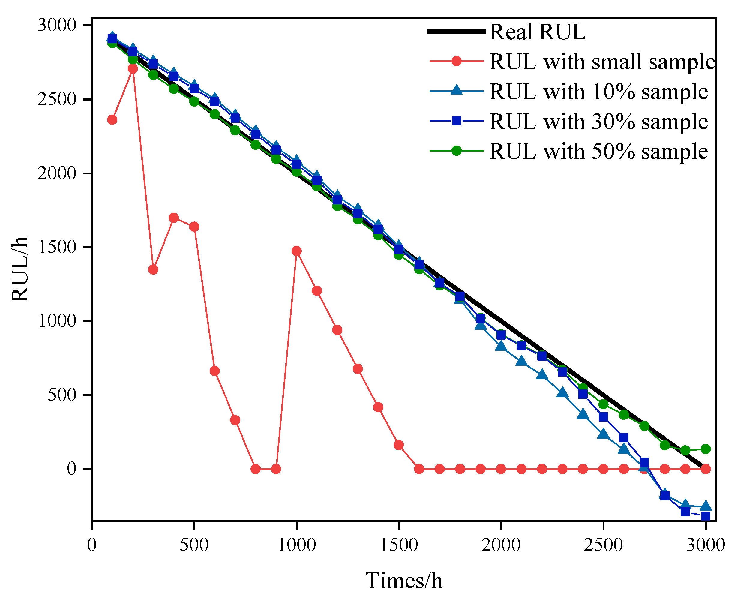
Considering the uncertainty induced by the oil small sample data, the multi-attribute representation architecture of indicator-attribute-state is proposed to realize the information fusion based on the probability membership, which forms the quantitative characterization of the state for RUL prediction.

(2)

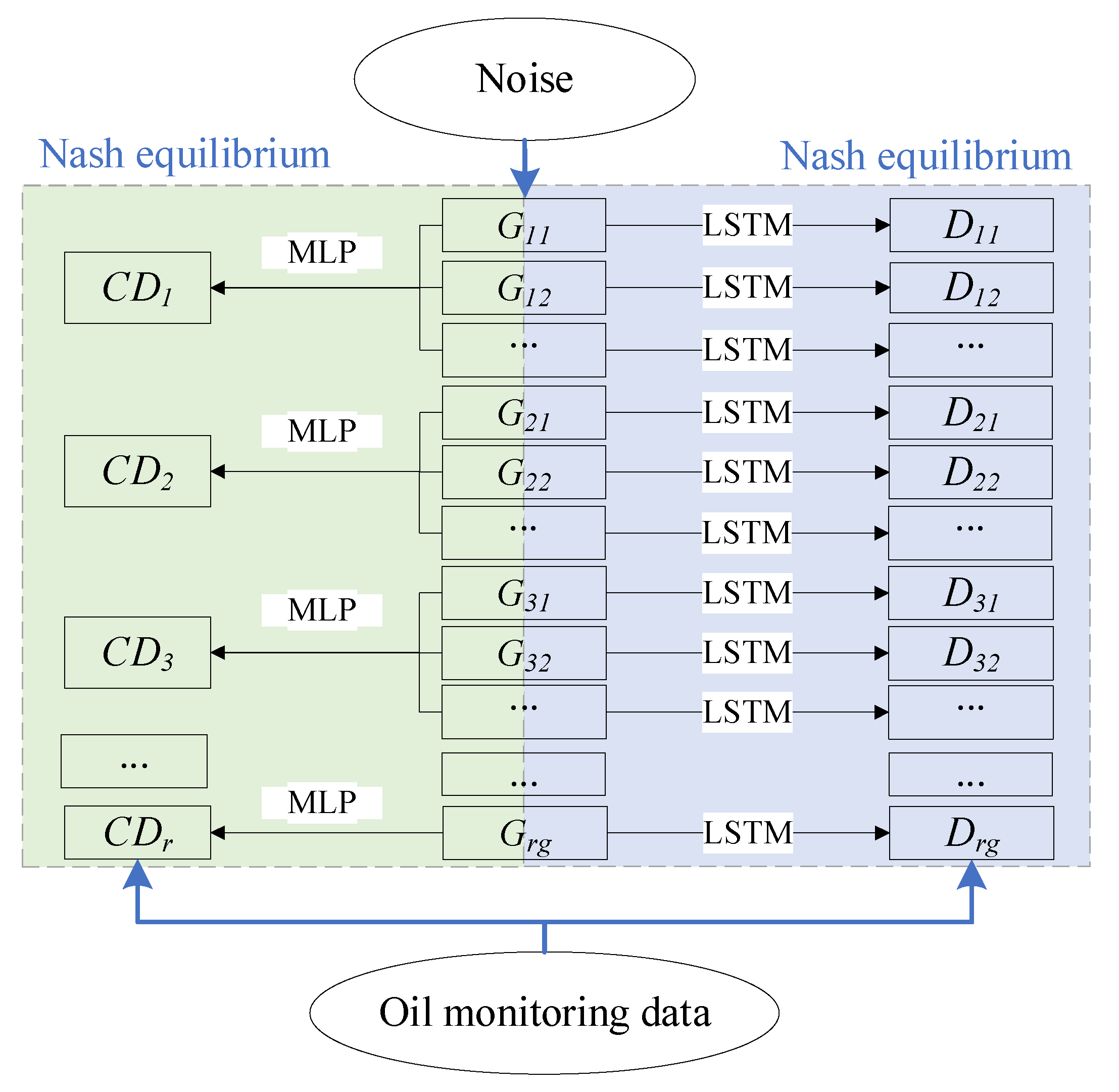
Regarding the interaction between monitoring indicators, a multi-attribute CMC-GAN is constructed to introduce indicator mutual constraints to realize data augmentation of multi-indicator monitoring data.

(3)

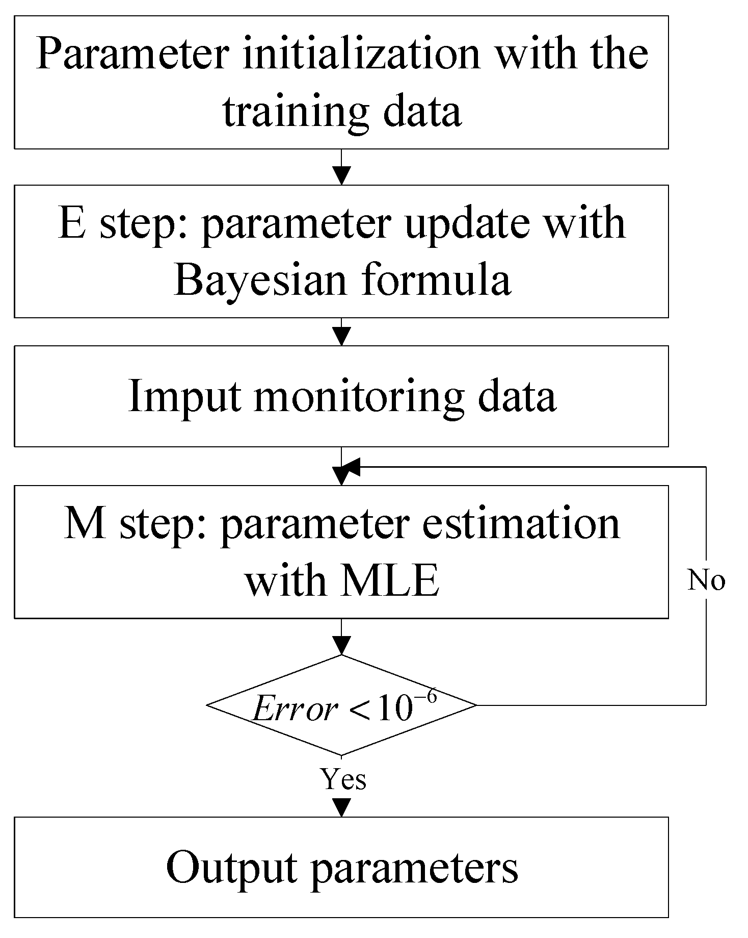
Via stochastic process to describe the comprehensive wear state, the parameter updating strategy is proposed based on EM to realize the RUL prediction under the multi-indicator data augmentation.

The rest of the paper is organized as follows: Section 2 proposes a multi-attribute wear state characterization methodology, Section 3 introduces an RUL modeling approach, Section 4 presents case studies, and Section 5 contains the conclusion.

2. Augmented Quantitative Characterization of Multi-Attribute Wear State

Since a single indicator cannot comprehensively capture wear characteristics, multi-indicator fusion can integrate different sources of detailed descriptions, which can provide richer support for decision-making. Therefore, a CMC-GAN is constructed to perform data augmentation for RUL prediction, and fuzzy probability is applied to integrate multi-attribute state fusion. First, the distributed representation architecture of indicator-attribute-state is built. It represents the mapping between the monitoring data and the state. Second, CMC-GAN is constructed based on the multi-attribute architecture, achieving the augmentation of the small-sample data. Finally, the fuzzy membership function is used to accomplish the multi-attribute evaluation, and then the comprehensive Health Indicator (HI) is obtained.

2.1. Basic Definition of Wear State Grade

To evaluate the wear state, the full range of wear state values is divided into corresponding intervals corresponding to ordered state classes. A probability distribution of indicators belonging to a state class can be calculated at each set. To quantitatively describe the wear state, the corresponding variables are defined.

(1)

Set of state grades: $H=\left\{H_1,H_2,\cdots ,H_c\cdots ,H_N\right\}$, $c=2,\cdots N$ where N is the number of state grade divisions,

(2)

Set of attributes of state: $A=\left\{A_1,A_2,\cdots ,A_i\cdots ,A_N\right\}$, $i=2,\cdots r$, where r is the number of attributes,

(3)

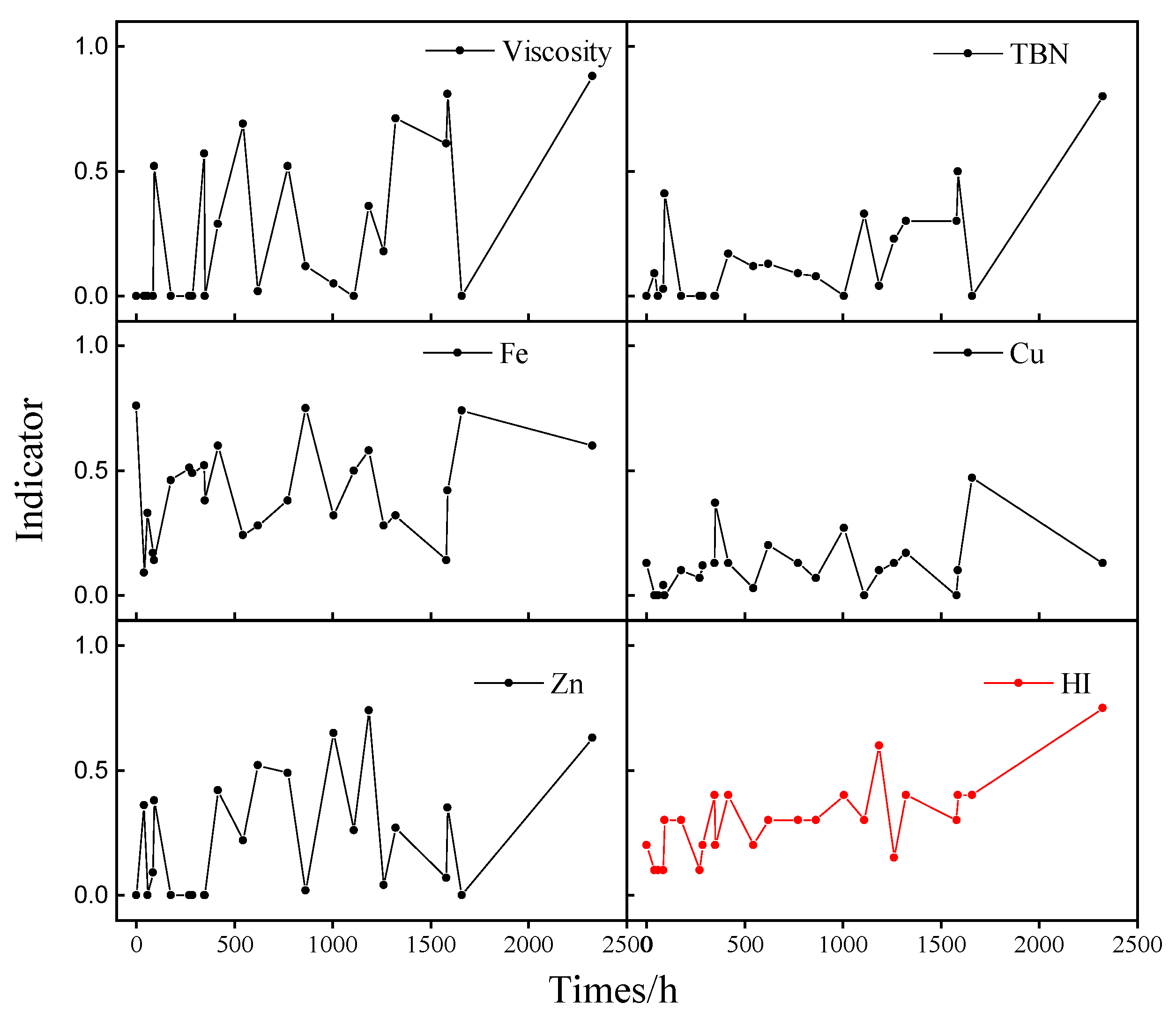
Set of indicators of state: $A_i=\left\{a_{i1},a_{i2},\cdots ,a_{ij}\cdots ,a_{ig}\right\}$, $j=2,\cdots g$, where g is the number of indicators contained in the i-th attribute.

Since different attributes can reflect the characteristics of a particular aspect of the wear state, the fusion of assessment with multiple attributes can comprehensively reflect the wear state. The relationship between the indicators, attributes, and states of the fluid state is shown in Figure 1. The probability-based model for quantitative characterization mainly includes indicator, attribute, and state layers. The indicator layer is the input layer, which can obtain the probability of the indicator belonging to the corresponding state grade by fuzzy assessment based on the monitoring data; the attribute layer is the bridging layer, which combines the probability of belonging to a particular state with the weighting of the corresponding indicator; the state layer is the output layer, which obtains the quantitative wear state value HI through the combination of the membership probability and the utility interval.

2.2. CMC-GAN Network Architecture

Let G be an MTS (Multivariate Time Series) dataset consisting of $r\times g$ instances, each of which contains r channels $X_i$, where $i\in 1,\dots ,r$. An example of G can be described as $G_{ni}=\left\{\left(G_1,\dots ,G_{nr}\right)\right\}$, and a distribution $q\left(G_1,\dots ,G_r\right)$ is searched for as close as possible to the real data distribution $p\left(G_1,\dots ,G_r\right)$. In a typical GAN framework, it may be challenging to find the optimal solution as the optimization objective depends on the number of channels, duration, and data distribution. Therefore, instead of using a separate generator G_i to learn the marginal distribution $p\left(G_i\right)$ for each channel $G_i$ individually, the central discriminator (CD_i) is simultaneously used to focus on the conditional distribution $p\left(G_i\left|G_{i\ne j}\right.\right)$, where $G_{\mathrm{i}\ne j}$ denotes all the channels except channel i. This approach ensures that the true correlations between the channels are preserved. A detailed description of the architecture is shown in Figure 2. A Gaussian white noise generator is constructed for each indicator $a_{ig}$, and the LSTM is constructed for each generator $G_{ig}$ and the discriminator $D_{ig}$. Consider the coupled correlation between indicators with uniform attribute $A_i$. These interactions are treated as CD_i. Each central channel constructs a multilayer perceptron (MLP) network with inputs of real monitoring data, while the attribute association of each channel is constrained by a CD. In this way, the data generated is based on random noise, which simultaneously considers the identification of single indicators and the constraints of attributes, guaranteeing the reliability of data generation. During the training process, when the minimum loss of D and CD is satisfied, i.e., the Nash equilibrium moment, the output of the acquired generated samples is the augmented samples.

The generator G_i and discriminator D_i of the GAN are composed of $r\times g$ long short-term memory neural networks (LSTMs), and the central discriminator CD_i contains r multilayer perceptron neural networks (MLPs). The optimization objective of the GAN is divided into the local objective of the generator and the central objective of the central channel, in which the local objective is to obtain the optimal parameter for estimating the marginal distribution $p\left(G_i\right)$ of each channel, i.e., for each channel i, it needs to be optimized as shown in Equation (1).

$$\underset{q}{\min }D\left(p\left(G_i\right)‖q\left(G_i\right)\right)$$

(1)

where D measures a distance metric between any two distributions. $q$ is the generator sample distribution, $p$ is the discriminator sample distribution, $G$ is the dataset, and each instance of $G$ contains r channels $G_i$, $G_i$ is the i-th channel, $i\in 1,\dots ,r$.The central objective is to estimate the conditional distribution of a channel, i.e., $p\left(X_i\left|X_{i\ne j}\right.\right)$ taking into account all other channels. Assume that the channels are independent of each other, the following constraints are constructed:

$$\underset{q}{\min }D\left({\displaystyle \prod _{i=1}^{r}p\left(G_i\left|G_{i\ne j}\right.\right)‖{\displaystyle \prod _{i=1}^{r}q\left(G_i\left|G_{i\ne j}\right.\right)}}\right)$$

(2)

When all generators $G_i$ share the initial random noise z, Equation (2) changes to

$$\underset{q}{\min }D\left({\displaystyle \prod _{i=1}^{r}p\left(G_i\left|z\right.\right)‖{\displaystyle \prod _{i=1}^{r}q\left(G_i\left|z\right.\right)}}\right)$$

(3)

Define global loss as a linear combination of the local target loss and the central target loss.

During the training process, the discriminator in the channel GAN, its pairwise generator, and the central discriminator will be trained against each other. The optimization objective function of single channel GAN with a central discriminator is shown in Equation (4)

$$\begin{array}{l}\underset{{\theta }_i}{\min } \underset{{\varphi }_i}{\max } \underset{\alpha }{\max }V\left(G_{i,{\theta }_i},D_{i,{\varphi }_i},{CD}_{\alpha }\right)={{\rm E}}_{x\sim P_{data}}\left[\log \left(D_{i,{\varphi }_i}\left(G_i\right)\right)+\gamma \log \left({CD}_{\alpha }\left(G\right)\right)\right]\\ \hspace{1em}\hspace{1em}\hspace{1em}\hspace{1em}\hspace{1em}\hspace{1em}\hspace{1em}\hspace{1em}\hspace{1em}\hspace{1em}\hspace{1em}\hspace{1em}\hspace{1em}+{{\rm E}}_{z\sim P_z}\left[\log \left(1-D_{i,{\varphi }_i}\left(G_{i,{\theta }_i}\left(z\right)\right)\right)+\gamma \log \left(1-{CD}_{\alpha }\left(G_{i,{\theta }_i}\left(z\right)\right),G_{j\ne i}\left(z\right)\right)\right]\end{array}$$

(4)

where $\theta$ is the parameter of the generative network, $\gamma$ is the central discriminator hyperparameter, $\varphi$ is the discriminator network parameter, $\alpha$ is the central discriminator hyperparameter, and z represents initial random noise.

2.3. Quantitative Characterization of Fuzzy Membership

As the dimensions and sizes of the data for the different indicators are inconsistent, the monitoring data need to be normalized by converting the other indicators to the same scale. The monitoring data are classified into benefit and cost indicators. Data with more extensive and better indicator values, such as Fe and Cu, are defined as benefit-type indicators; data with smaller and better indicator values, such as Zn content, are defined as cost-type indicators, which are normalized by applying Equation (5).

$${\overline{x}}_{ij}=\left\{\begin{array}{c}{\displaystyle \frac{x_{is}-x_{ij}}{x_{is}-x_{i0}}}\begin{array}{cc},& x_{ij}\in I_1\end{array}\\ {\displaystyle \frac{x_{ij}-x_{i0}}{x_{is}-x_{i0}}}\begin{array}{cc},& x_{ij}\in I_2\end{array}\end{array}\right.$$

(5)

where $x_{is}$ denotes the failure threshold represented by indicator $x_{ij}$, the $x_{is}$ denotes set value can be referred to as the failure value specified in the oil change standard [21], $x_{i0}$ denotes the initial value of indicator $a_{ij}$, the setting of which can be referred to the new indicator, ${\overline{x}}_{ij}$ denotes normalized indicator data, $I_1$ represents cost-type indicator set, $I_2$ represents benefit-type indicator set.

Fuzzy probability can deal with data uncertainty, providing stability and adaptability to each indicator characterization. To express the mapping relationship between the indicator data and the wear state grade, the fuzzy membership function shown in Equation (6) is applied to calculate the degree, i.e., the membership degree ${\beta }_{H_c}$, that the normalized indicator value ${\overline{x}}_{ij}$ belongs to the state grade of $H_c$.

$${\beta }_{H_c}\left({\overline{x}}_{ij}\right)=\exp \left(-{\left({\displaystyle \frac{{\overline{x}}_{ij}-\mu }{\sigma }}\right)}^2\right)$$

(6)

where $\mu$ and $\sigma$ denote the mean and standard deviation of the Gaussian affiliation function, ${\beta }_{H_c}\left({\overline{x}}_{ij}\right)$ represents the probability of affiliation of the normalized indicator ${\overline{x}}_{ij}$ to the grade $H_c$.

Multiple indicators that reflect the same feature jointly construct the attributes, and all the attributes jointly determine the wear state. To characterize the attribute evaluation, the weighted multi-indicator assessment can obtain the membership probability of the attribute corresponding to the state grade, as shown in Equation (7), assuming that the probability of the attribute j belonging to the $H_c$ grade is known.

$${\beta }_{H_c}\left(A_i\right)=w_{ij}{\beta }_{H_c}\left({\overline{x}}_{ij}\right)$$

(7)

where ${\beta }_{H_c}\left(A_i\right)$ denotes the probability that the i-th attribute belongs to grade $H_c$, and $w_{ij}$ is the weight of the j-th indicator in the i-th attribute.

Equation (7) indicates the probability of the wear state belonging to a certain state grade. To provide a quantitative output of the wear state characterization, the utility intervals are applied to assign the membership probability [22]. ${\beta }_{H_c}\left({\overline{x}}_{ij}\right)$ denotes the membership probability of the likelihood that ${\overline{x}}_{ij}$ belongs to $H_c$, which corresponds to all of the wear state grades $H=\left\{H_1,H_2,\cdots ,H_c\cdots ,H_N\right\}$. It is assumed that the utility intervals of the assessment state class $H_c$ are $\mu \left(H_c\right)$, and they need to be trained through the monitoring data [23]. Considering that the information is complete in the assessment, the quantitative output of the wear state is simplified to obtain Equation (8)

$$\mathrm{HI}=\sum _{c=1}^N\sum _{i=1}^r{\beta }_{H_c}\left(A_i\right)\mu \left(H_c\right)$$

(8)

Based on the above calculations, we perform small-sample oil information augmentation by CMC-GAN and apply fuzzy membership probability to achieve a quantitative characterization of the wear state, which outputs the quantified value of the wear state, HI.

3. Modeling for RUL Prediction

Accurate indicator construction guarantees RUL prediction. Thus, joint CMC-GAN and fuzzy membership probability assignment are used for oil multi-indicator fusion. Next, the HI serves as an input for RUL prediction modeling. First, the oil degradation process is modeled using the Wiener process. Second, to obtain dynamically updated parameters, an EM algorithm combined with a priori parameter is proposed for real-time parameter estimation. Finally, the life prediction is performed based on the updated model parameters.

3.1. Wear State Modelling

The Wiener process provides a strong expression of uncertainty by introducing the Brownian motion to describe the stochastic volatility. Its general form describes the system uncertainty through two parameters, the drift coefficient and the diffusion coefficient, where the drift coefficient describes the decay trend and the diffusion term is used to characterize the volatility, and the mathematical expression is

$$x_i=x_0+a_{i}t+w_i$$

(9)

where $x_i$ denotes the monitoring data of the system at the moment i, $x_0$ denotes the initial state, $a_i$ is the drift coefficient, $w_i$ is the diffusion system, based on the definition of the Wiener process, $a_i$ obeys the normal distribution with the mean ${\mu }_0$ and the variance ${\sigma }_0^2$, and $w_i$ obeys the distribution with the mean of 0 and the variance of ${\sigma }^2$.

3.2. Parameter Updates

There are two variables $a_i$ and $w_i$ in Equation (9), which can be used for parameter estimation by maximum likelihood estimation when the sample size is a historical sample. However, dynamic updating of the model parameters is required when considering the real-time sample generation on the model parameters.

For the monitoring sample dataset $\left\{x_i,i=1,2,\cdots ,K\right\}$, the smoothed data series $\left\{x_i-x_{i-1}-a_{i-1}{\mathsf{\Delta }t}_{i-1}, i=1,2,\cdots ,K\right\}$ obeys the following probability distribution:

$$P\left(X_{1:K}\right)a_i={\displaystyle \frac{1}{{\displaystyle \prod _{j=1}^k\sqrt{2\pi {\sigma }^2\left(t_j-t_{j-1}\right)}}}}\exp \left[-\sum _{j=1}^k{\displaystyle \frac{{\left(x_j-x_{j-1}-a_i\left(t_j-t_{j-1}\right)\right)}^2}{2{\sigma }^2\left(t_j-t_{j-1}\right)}}\right]$$

(10)

By constructing the PDF based on Equation (9), a sequence of serial observations $\left\{\left(x_i-x_{i-1}\right)/{\mathsf{\Delta }t}_{i-1}, i=1,2,\cdots ,K\right\}$ can be obtained, which obeys the following probability distribution:

$$P\left(x\right)={\displaystyle \frac{1}{\sqrt{2\pi {\sigma }_0^2}}}\exp \left[-{\displaystyle \frac{{\left(x-\mu \right)}^2}{2{\sigma }_0^2}}\right]$$

(11)

After constructing the probability density functions for the parameters $a_i$ and $w_i$, the EM algorithm is applied to update the parameters. Considering the hyperparameters $a~N({\mu }_0,{\mathsf{\sigma }}_0^2)$ and $w~N(0,{\sigma }^2)$ involves in the estimation of the sample data, the parameters of Equations (10) and (11) are represented by ${\theta }_k=[{\mu }_{0,k},{\mathsf{\sigma }}_{0,k}^2,{\mathsf{\sigma }}_k^2]$. Subsequently, the subsequent evaluation of the model parameters ${\theta }_k$ is updated based on the observation. The construction of the E-steps and M-steps in the EM algorithm is shown below.

E-step: Construct the expected posterior probability from the Bayesian formula.

$$P\left({\mu }_0,{\mathsf{\sigma }}_0^2,{\sigma }^2|X_{1:k}\right)={\displaystyle \frac{P\left(X_{1:k}|{\mu }_0,{\mathsf{\sigma }}_0^2,{\sigma }^2\right)P\left({\mu }_0,{\mathsf{\sigma }}_0^2\right)}{P\left(X_{1:k}\right)}}\propto P\left(X_{1:k}|{\mu }_0,{\mathsf{\sigma }}_0^2,{\sigma }^2\right)P\left(X_{1:k}|{\mu }_0,{\mathsf{\sigma }}_0^2\right)$$

(12)

Equation (12) represents the joint probability density obeying a normal distribution, whose expectation and variance can be solved analytically to construct an iterative formula as shown in Equation (13)

$$\begin{array}{l}{\hat{\mu }}_{0,k}^{i+1}={\displaystyle \frac{{\mu }_0{\sigma }^2+{\overline{x}}_k{\sigma }_0^2}{t_k{\sigma }_0^2+{\sigma }^2}}\\ {{\hat{\sigma }}_{0,k}^2}^{i+1}={\displaystyle \frac{{\sigma }_0^2{\sigma }^2}{t_k{\sigma }_0^2+{\sigma }^2}}\end{array}$$

(13)

M-step: Parameter iteration by maximum likelihood estimation,

$${\hat{\mathsf{\Theta }}}_k^{i+1}=\arg \max \left(\ln \left({\mathsf{\Theta }|\hat{\Theta }}_k^i\right)\right)$$

(14)

where ${\mathsf{\Theta }}_k=[{\mu }_{0,k},{\mathsf{\sigma }}_{0,k}^2,{\mathsf{\sigma }}_k^2]$ denotes the a priori parameter information obtained by the k-th monitoring point based on the calculation of historical training samples, ${\hat{\Theta }}_k=[{\hat{\mu }}_{0,k},{\hat{\sigma }}_{0,k}^2,{\hat{\sigma }}_k^2]$ denotes the parameter information updated by the kth monitoring point, and i denotes the current iteration step.

Bayesian updating of the model parameters ${\mu }_0, {\mathsf{\sigma }}_0^2$ is performed using maximum likelihood estimation for the parameters ${\mathsf{\sigma }}_k^2$ as follows

$$\begin{array}{l}\ln P\left(X_{1:k},{\mu }_0,{\mathsf{\sigma }}_0^2,{\sigma }^2|{\theta }_k\right)=\ln P\left(X_{1:k}|{\mu }_0,{\mathsf{\sigma }}_0^2,{\sigma }^2,{\theta }_k\right)+\ln P\left({\mu }_0,{\mathsf{\sigma }}_0^2|{\theta }_k\right)\\ \hspace{1em}\hspace{1em}\hspace{1em}\hspace{1em}\hspace{1em}\hspace{1em}\hspace{1em}\hspace{1em} =-{\displaystyle \frac{k+1}{2}}\ln 2\pi -k\ln \sigma -{\displaystyle \frac{1}{2}}\ln {\displaystyle \sum _{j=1}^k\left(t_j-t_{j-1}\right)}\\ \hspace{1em}\hspace{1em}\hspace{1em}\hspace{1em}\hspace{1em}\hspace{1em}\hspace{1em}\hspace{1em} -\sum _{j=1}^k{\displaystyle \frac{{\left(x_j-x_{j-1}-b\left(t_j-t_{j-1}\right)\right)}^2}{2{\sigma }^2\left(t_j-t_{j-1}\right)}}-k\ln {\sigma }_{0,k}-{\displaystyle \frac{{\left(x-{\mu }_{0,k}\right)}^2}{2{\sigma }_{0,k}^2}}\end{array}$$

(15)

For the parameter maximum likelihood estimation, Equation (15) is solved using the gradient descent method, and the parameter ${\sigma }^2$ update is obtained as

$${\left({\sigma }_k^2\right)}^{i+1}={\displaystyle \frac{1}{k}}\sum _{j=1}^k{\displaystyle \frac{{\left(x_j-x_{j-1}\right)}^2-2{\mu }_{0,k}\left(x_j-x_{j-1}\right)\left(t_j-t_{j-1}\right)+{\left(t_j-t_{j-1}\right)}^2\left({\mu }_{0,\mathrm{k}}^2+{\sigma }_{0,\mathrm{k}}^2\right)}{\left(t_j-t_{j-1}\right)}}$$

(16)

here the initial values of ${\mu }_0$ and ${\sigma }_0^2$ can be obtained by calculating the mean and variance of the sequence $\left\{a_i=x_i/t_i, i=1,2,3,\dots ,K\right\}$.

Therefore, the updated model parameter estimates ${\widehat{\Theta }}_k=[{\widehat{\mu }}_{0,k},{\widehat{\sigma }}_{0,k}^2, {\widehat{\sigma }}_k^2]$ can be obtained. The detailed iteration steps for updating are illustrated in Figure 3.

Combining the updated parameter estimates ${\widehat{\Theta }}_k=[{\widehat{\mu }}_{0,k},{\widehat{\sigma }}_{0,k}^2,{\widehat{\sigma }}_k^2]$, the failure threshold of the fluid is defined as D. Assuming that the moment when the state reaches D is T_D, the variable t in Equation (9) is solved, and the RUL of the fluid at time t is expressed as:

$$l=T_D-T=\left(D-x_t\right)/{\widehat{\mu }}_{0,k}$$

(17)

where l is the remaining effective life, t is the current monitoring moment, and $x_t$ is the current state.

4. Case Study

4.1. Case 1

To evaluate the prediction performance of the CMC-GAN method under varying training data sizes, three sets of comparison experiments have been conducted for the Fe content indicator based on the proposed model. The experiments use 10%, 30%, and 50% of the sample data for sensitivity analysis. The data generation and RUL prediction are performed by applying the CMC-GAN shown in

Table 1. Data generating steps of Multi-Channel GAN Model.

Step	Process
Step 1	Apply LSTM to construct generators and discriminators of GAN networks;
Step 2	Take a random noise vector as the input of generator, which maps through a fully connected layer (Linear layer) to the target data space to output the final data sequence, the loss function is selected as the binary cross entropy loss;
Step 3	The input of the discriminator is a sequence of real data and a sequence of data generated by the generator, which is mapped to a single output node through multiple LSTM fully connected layers, using a binary cross-entropy loss to assure that the prediction of the real data is close to 1, and the prediction of the generated data is close to 0;
Step 4	The central discriminator receives the fusion of time series generated by all channel generators as a multivariate time series, which is structured as a Linear layer, a LeakyReLU activation function and a Dropout layer;
Step 5	Import the simulation sample sequence and train the objective function optimization based on Equation (4) until $\left|L_t-L_{t-1}\right|\le \epsilon$ finish training, $\epsilon ={10}^{-6}$;
Step 6	Apply Equations (13)–(16) to estimate the trajectory parameters for the control guided model, and obtain the model temporal parameter set ${\widehat{\theta }}_k=\left[{\widehat{\mu }}_{0,k},{\widehat{\sigma }}_{0,k}^2,{\widehat{\sigma }}_k^2\right]$;
Step 7	Substitute the updated parameter expectations into Equation (17) to obtain the trajectory tracking data.

.

Each experiment has been repeated 30 times, and the resulting indicators are statistically analyzed, as presented in

Table 2. Fe content prediction based on CMC-GAN.

Number	RUL	Real Data of Fe	10% Predicted Data of Fe	30% Predicted Data of Fe	50% Predicted Data of Fe
	h	ppm	ppm	ppm	ppm
1	290	15.40	12.61	13.87	18.27
2	280	15.95	12.86	13.98	18.25
3	270	16.33	13.32	14.24	18.25
4	260	17.08	13.96	14.69	18.32
5	250	17.95	14.73	15.32	18.49
6	240	18.79	15.59	16.12	18.80
7	230	18.98	16.54	17.04	19.24
8	220	19.59	17.55	18.03	19.77
9	210	20.33	18.59	19.04	20.39
10	200	21.32	19.60	20.04	21.08
11	190	22.08	20.57	21.00	21.84
12	180	22.31	21.50	21.95	22.69
13	170	23.43	22.47	22.93	23.62
14	160	24.30	23.52	23.96	24.62
15	150	24.83	24.72	25.07	25.67
16	140	25.94	26.06	26.26	26.71
17	130	26.78	27.48	27.45	27.72
18	120	28.10	28.94	28.59	28.67
19	110	28.40	30.36	29.62	29.58
20	100	29.20	31.74	30.57	30.49
21	90	30.54	33.10	31.51	31.45
22	80	32.04	34.47	32.56	32.49
23	70	33.18	35.88	33.81	33.62
24	60	34.04	37.35	35.37	34.82
25	50	35.16	38.92	37.25	36.03
26	40	36.75	40.57	39.42	37.20
27	30	38.14	42.24	41.72	38.27
28	20	38.65	43.80	43.91	39.19
29	10	40.24	45.04	45.65	39.88
30	0	42.14	45.74	46.62	40.24

.

Table 2 shows a significant error between the predicted and actual values when using only 10% of the training data. This indicates that too few training samples do not allow the generator to fully learn the degradation characteristics of the full cycle of the lubricating oil. When the training samples are increased to 30%, the prediction accuracy is improved, but there is still a certain error compared with 50% samples. This indicates that augmenting the training set size can improve the modeling capability of the CMC-GAN. The prediction results match the real values when using 50% samples for training. This fully verifies that larger training samples are conducive to improving the generalization ability of CMC-GAN.

The augmented data generated by the CMC-GAN are used as input to the RUL prediction model for parameter updating. The updated parameters are then substituted into Equation (17) to calculate the oil RUL. The results are presented in Figure 4.

It can be seen from Figure 4 that the prediction values generated by CMC-GAN can be closer to the real data, which is significantly better than the prediction results using only the original small-sample data. This fully demonstrates the effectiveness of the CMC-GAN method in solving the data scarcity problem. With the generator G training, CMC-GAN can learn the degradation characteristics of the lubricant full cycle from the limited monitoring data and then generate samples that are highly consistent with the real cases. These augmented samples not only increase the size of the training set but also improve the diversity of the data.

4.2. Case 2

To verify the effectiveness of the proposed method, the data of four engineering vehicles with continuous real-time operation of more than 2000 h are selected. The monitoring object is mainly the wear information in lubricating oil, which is regularly sampled and tested offline for five key indicators: viscosity, Total Alkali Number (TBN) value, Fe, Cu, and Zn. The monitoring data came from field tests over more than 1.5 years. One of the typical monitoring data is in Figure 5.

The raw data of each monitoring indicator are normalized and set to a dimensionless range of 0–1, as shown in Figure 5. It can be seen that the five monitoring indicators show strong heterogeneity characteristics. Therefore, a single indicator cannot fully reflect the overall state variability of the oil. Consistent results cannot be obtained based on the single indicator RUL prediction. Therefore, the comprehensive health indicator (HI) model of Equation (8) is applied to integrate these five indicators. By optimizing the training of the model parameters, the HI indicators reflecting the degradation of the integrated wear state are obtained.

To evaluate the effectiveness of the HI indicator in the degradation model, the five indicators are evaluated for trendiness by the Spearman correlation coefficient $T{r}_n$ [19]:

$$T{r}_n={\displaystyle \frac{\left|{\displaystyle \sum _{k=1}^K\left(t_k^{\ast }-{\overline{t}}^{\ast }\right)\left(x_{n,k}^{\ast }-{\overline{x}}_n^{\ast }\right)}\right|}{\sqrt{{\displaystyle \sum _{k=1}^K{\left(t_k^{\ast }-{\overline{t}}^{\ast }\right)}^2{\left(x_{n,k}^{\ast }-{\overline{x}}_n^{\ast }\right)}^2}}}}$$

(18)

where $\left\{t_k^{\mathrm{*}}, k=1,2,\dots ,K\right\}$ and $\left\{x_{n,k}^{\mathrm{*}}, k=1,2,\dots ,K\right\}$ denote the time series corresponding to sampling and the time series corresponding to the nth indicator observation, $\left\{n=1,2,\dots ,6\right\}$, $t^{\mathrm{*}}$ and $x_n^{\mathrm{*}}$ denote the means of $\left\{t_k^{\mathrm{*}}, k=1,2,\dots ,K\right\}$ and $\left\{x_{n,k}^{\mathrm{*}}, k=1,2,\dots ,K\right\}$.

The larger Spearman correlation coefficient $T{r}_n$ indicates the better monotonic trend of the feature. The calculation results are shown in

Table 3. Spearman coefficient $T{r}_n$ calculation for oil monitoring with multiple indicators.

Indicator	Viscosity	TBN	Fe	Cu	Zn	HI
$T{r}_n$	0.45	0.82	0.35	0.30	0.65	0.85

.

As shown in Table 3, the integrated health indicator HI has a maximum Spearman correlation coefficient of 0.85, indicating that it presents a strong monotonic correlation with the actual wear state, which demonstrates that the HI indicator can reflect the oil degradation tendency better and further verifies the superiority of the proposed method.

During the process of parameter estimation, the parameters are updated along with the oil monitoring data, and the parameters of the model for the engine oil are updated, as shown in Figure 6.

The dynamic iteration using the drift term a_i of WPM is adopted in Figure 6, which realizes the update of the decay rate. It can be seen that drift and diffusion coefficients converge with increasing update samples. The stochastic fluctuation term has been treated as a perturbation factor, which is equivalent to filtering the monitoring data. The random fluctuation of the wear state is effectively captured, enhancing the accuracy and robustness of RUL prediction. The results of oil RUL prediction based on single and integrated HI indicators are shown in Figure 7, and Cu is excluded from the comparison since it has a similar $T{r}_n$ to Fe. The upper row shows the comparison methods for data processing, including the FIS fusion and Selection fusion [19].

It can be seen from Figure 7 that the HI indicator is more consistent with the actual decay process than a single indicator, which is more suitable for RUL prediction. The CRA is calculated to evaluate the accuracy of the prediction, which a value closer to 1 indicates better performance [20]. The definition of CAR is shown as

$$\mathrm{CRA}={\displaystyle \frac{1}{K}}\sum _{k=1}^K\left(1-{\displaystyle \frac{\left|{\widehat{l}}_k-l_k\right|}{l_k}}\right)$$

(19)

where K is the length of the sample sequence; ${\widehat{l}}_k$ and $l_k$ represent the predicted and the actual value at moment $t_k$, respectively.

CARs for RUL prediction from nine different indicators are shown in

Table 4. CARs of prediction with different methods.

Indicator Type	Data Processing	Test-1	Test-2	Test-3	Test-4
Fusion method	FIS fusion	0.7134	0.3356	0.4802	0.4372
	Selection fusion	0.3589	0.7188	0.2729	0.4852
	CMC-GAN	0.9765	0.9343	0.9927	0.9215
Single indicator	Viscosity	0.2617	0.4441	0.3321	0.4263
	TBN	0.3112	0.5493	0.1608	0.6980
	Fe	0.3778	0.6299	0.6336	0.3588
	Zn	0.3290	0.4403	0.6983	0.3289

. It can be seen that the higher CARs are obtained in the proposed method for all four sets of full-life assessment tests. For individual monitoring indicators, poor indicator monotonicity and tendency severely limit the RUL prediction accuracy, resulting in a single indicator being unavailable for oil RUL prediction.

To quantitatively evaluate the accuracy of the RUL prediction, the error percentage of the prediction ${Error}_n=\left(l_n-{\widehat{l}}_n\right)/l_n$ is computed, where $l_n$ and ${\widehat{l}}_n$ represent the real and predicted RUL of the n-th sample, respectively. The percentage of error is substituted into the following evaluation indexes of accuracy to obtain a comprehensive score

$$\begin{array}{cc}Score={\displaystyle \frac{1}{N}}{\displaystyle \sum _{n=1}^N{A}_n},& A_n=\left\{\begin{array}{c}\begin{array}{cc}\exp \left(-\ln \left(0.5\right)\left({\displaystyle \frac{100Erro{r}_n}{5}}\right)\right),& \begin{array}{ll}if& Erro{r}_n\le 0\end{array}\end{array}\\ \begin{array}{cc}\exp \left(+\ln \left(0.5\right)\left({\displaystyle \frac{100Erro{r}_n}{20}}\right)\right),& \begin{array}{cc}if& Erro{r}_n\ge 0\end{array}\end{array}\end{array}\right.\end{array}$$

(20)

In the validation of the engineering vehicle operating data, 10 maintenance times are randomly selected for RUL prediction, and the results are shown in

Table 5. The accuracy scores of PHM by RUL prediction.

Times/h	Real RUL/h	Predicted RUL with HI/h	Predicted RUL with Viscosity/h	Predicted RUL with TBN/h	Predicted RUL with Fe/h	Predicted RUL with Zn/h
1500	2200	1747	3188	2992	3082	2086
2000	1700	1673	1573	2475	678	1884
1700	2000	1699	697	1649	1474	1378
2200	1500	1631	2116	2962	162	2207
400	3300	4017	3708	4323	3290	4750
2500	1200	1727	909	2034	0	3378
1600	2100	1805	3018	3192	0	2455
700	3000	3138	3367	3709	1931	4960
1000	2700	2940	1957	2711	1350	4814
3100	600	764	0	1663	0	2208
Score		0.3837	0.2096	0.1550	0.2127	0.1499
Std (Error%)		20.46	48.39	54.86	47.66	91.33

. Considering the failure risk in PHM when the predicted RUL is larger than the real RUL, namely ${Error}_n\le 0$, a larger penalty weight will be given in the scoring process based on the principle of caution maintenance. The RULs obtained from the computation in 10 random sets of maintenance times are given in Table 5, and a comparison of Scores and error percentages reveals that RUL prediction of oil by applying HI can provide optimal decision making for maintenance.

5. Conclusions

To accurately characterize the lubricant state and improve the RUL prediction accuracy, this research employs a multi-channel GAN to realize lubricant sample data augmentation. Fuzzy probabilistic fusion of oil multi-indicator information is applied to obtain comprehensive health indicators to reflect the wear state comprehensively. To obtain accurate RUL prediction, the RUL prediction model is established using the integrated health indicators. The results demonstrate better prediction under small-sample conditions. The main conclusions are as follows.

1.

CMC-GAN is adopted to achieve the augmentation of oil small-sample data and the HI indexes of joint multi-attribute quantitative characterization can comprehensively reflect the integrated wear state, guaranteeing the accuracy of RUL prediction.

2.

The model is constructed based on the Wiener process with the EM algorithm for parameter update, reflecting the gradual degradation trend of the wear state, which more accurately predicts the oil RUL.

3.

The proposed method shows superior performance through a real case study. It can be seen that the HI has the best monotonic trend by calculating $T{r}_n$, which provides the guarantee for RUL prediction.

There are still some limitations in the proposed method, in which the multi-indicator modeling is proposed as the data-driven model. However, reliable RUL prediction faces two challenges: (1) the prediction interpretability and (2) the robustness of the method; the proposed method relies on the selected condition, assuming that the wear mechanism is known. Thus, this limits the practicality of the proposed method. Therefore, we will focus on the interpretability of the model to improve its robustness.

References

- Pan, Y.; Han, Z.; Wu, T.; Lei, Y. Remaining Useful Life Prediction of Lubricating Oil with Small Samples. IEEE Trans. Ind. Electron. 2023, 70, 7373–7381. [Google Scholar] [CrossRef]
- Liu, Z.; Wang, H.; Hao, M.; Wu, D. Prediction of RUL of Lubricating Oil Based on Information Entropy and SVM. Lubricants 2023, 11, 121. [Google Scholar] [CrossRef]
- Wang, S.; Tian, Y.; Hu, X.; Wang, J.; Han, J.; Liu, Y.; Wang, J.; Wang, D. Identification of Grinding Wheel Wear States Using AE Monitoring and HHT-RF Method. Wear 2025, 562–563, 205668. [Google Scholar] [CrossRef]
- Wang, Y.; E, S.; Yang, K.; Xie, B.; Lu, F. Reliability-Based Robust Design Optimization with Fourth-Moment Method for Ball Bearing Wear. Lubricants 2024, 12, 293. [Google Scholar] [CrossRef]
- Morgan, I.; Liu, H.; Tormos, B.; Sala, A. Detection and Diagnosis of Incipient Faults in Heavy-Duty Diesel Engines. IEEE Trans. Ind. Electron. 2010, 57, 3522–3532. [Google Scholar] [CrossRef]
- Stein, G.J.; Randall, R.B. Vibration-Based Condition Monitoring (Industrial, Aerospace and Automotive Applications). Stroj. Cas. 2011, 62, e977668. [Google Scholar]
- Matania, O.; Bachar, L.; Bechhoefer, E.; Bortman, J. Signal Processing for the Condition-Based Maintenance of Rotating Machines via Vibration Analysis: A Tutorial. Sensors 2024, 24, 17. [Google Scholar] [CrossRef]
- Tambadou, M.S.; Chao, D.; Duan, C. Lubrication Oil Anti-Wear Property Degradation Modeling and Remaining Useful Life Estimation of the System Under Multiple Changes Operating Environment. IEEE Access 2019, 7, 96775–96786. [Google Scholar] [CrossRef]
- Wei, L.; Duan, H.; Jia, D.; Jin, Y.; Chen, S.; Liu, L.; Liu, J.; Sun, X.; Li, J. Motor oil condition evaluation based on on-board diagnostic system. Friction 2020, 8, 95–106. [Google Scholar] [CrossRef]
- Wang, W.; Hussin, B. Plant residual time modelling based on observed variables in oil samples. J. Oper. Res. Soc. 2009, 60, 789–796. [Google Scholar] [CrossRef]
- Makis, V.; Wu, J.; Gao, Y. An application of DPCA to oil data for CBM modeling. Eur. J. Oper. Res. 2006, 174, 112–123. [Google Scholar] [CrossRef]
- Liu, B.; Zhao, X.; Liu, G.; Liu, Y. Life cycle cost analysis considering multiple dependent degradation processes and environmental influence. Reliab. Eng. Syst. Saf. 2020, 197, 106784. [Google Scholar] [CrossRef]
- Özcan, M.M.; Kutbay, U. Improving Predictive Maintenance Performance in Limited Data Environment with CGAN. In Proceedings of the 2024 9th International Conference on Computer Science and Engineering (UBMK), Antalya, Turkiye, 26–28 October 2024; pp. 1–6. [Google Scholar] [CrossRef]
- He, X.; Ding, C.; Qiao, F.; Shi, J. An Incremental Remaining Useful Life Prediction Method Based on Wasserstein GAN and Knowledge Distillation. In Proceedings of the 2024 IEEE International Conference on Systems, Man and Cybernetics (SMC), Kuching, Malaysia, 7–10 October 2024; pp. 3857–3862. [Google Scholar] [CrossRef]
- Urban, A.; Zhe, J. A microsensor array for diesel engine lubricant monitoring using deep learning with stochastic global optimization. Sens. Actuators A Phys. 2022, 343, 113671. [Google Scholar] [CrossRef]
- Wang, W.; Hussin, B.; Jefferis, T. A case study of condition based maintenance modelling based upon the oil analysis data of marine diesel engines using stochastic filtering. Int. J. Prod. Econ. 2012, 136, 84–92. [Google Scholar] [CrossRef]
- Vališ, D.; Žák, L.; Pokora, O.; Lánský, P. Perspective analysis outcomes of selected tribodiagnostic data used as input for condition based maintenance. Reliab. Eng. Syst. Saf. 2016, 145, 231–242. [Google Scholar] [CrossRef]
- Vališ, D.; Forbelská, M.; Vintr, Z.; La, Q.T.; Leuchter, J. Perspective estimation of light emitting diode reliability measures based on multiply accelerated long run stress testing backed up by stochastic diffusion process. Measurement 2023, 206, 112222. [Google Scholar] [CrossRef]
- Pan, Y.; Wu, T.; Jing, Y.; Han, Z.; Lei, Y. Remaining useful life prediction of lubrication oil by integrating multi-source knowledge and multi-indicator data. Mech. Syst. Signal Process. 2023, 191, 110174. [Google Scholar] [CrossRef]
- Pan, Y.; Jing, Y.; Wu, T.; Kong, X. Knowledge-based data augmentation of small samples for oil condition prediction. Reliab. Eng. Syst. Saf. 2022, 217, 108114. [Google Scholar] [CrossRef]
- Hönig, V.; Procházka, P.; Obergruber, M.; Kučerová, V.; Mejstřík, P.; Macků, J.; Bouček, J. Determination of Tractor Engine Oil Change Interval Based on Material Properties. Materials 2020, 13, 5403. [Google Scholar] [CrossRef]
- Pan, Y.; Wu, T.; Jing, Y.; Wang, P. Multiattribute Modeling for Oil Condition Assessment Considering Uncertainties. IEEE Trans. Instrum. Meas. 2022, 71, 3509908. [Google Scholar] [CrossRef]
- Xu, F.; Yang, S.; Liang, B. Interval set-membership estimation for continuous linear systems. Int. J. Robust Nonlinear Control. 2020, 30, 5305–5321. [Google Scholar] [CrossRef]