Contact Load Calculation Models for Finite Line Contact Rollers in Bearing Dynamic Simulation Under Dry and Lubricated Conditions

Abstract

The key to exploring the behavior of bearings through dynamic methods lies in establishing an accurate model for calculating the contact load between the roller and the raceway. Based on the half-space theory of Boussinesq, this study developed a full-order model for calculating the contact load of the finite line contact roller. The model adopted an iterative procedure to calculate the contact load of each roller slice according to deformations. According to the comparisons between the contact loads obtained by the proposed model and those obtained by FEA, the average error for a cylindrical roller was approximately 2%, while that for a tapered roller was approximately 17%. By neglecting the influences of inter-slice contact stresses on the deformation of local roller slice, a fast-calculating method for the full-order model was developed, thereby reducing the calculation time by approximately 77%. By integrating the fast method with the Dowson–Higginson’s formula, another model was developed to calculate the contact load under lubrication conditions. The proposed models were utilized to investigate the dynamic characteristics of a double-row tapered roller bearing, and the results were validated through experiments. The proposed method could be utilized to assess dynamic performances of bearings across different operating scenarios.

1. Introduction

Bearings play very crucial roles in mechanical rotating systems, and proper operation of the system relies heavily on the optimal conditions of the bearings. Surface defects of the rotating elements and inadequate lubrication are critical factors that impact the operational condition of bearings. Surface defects can result in additional loads and induce forced vibrations within the support system, while insufficient lubrication can lead to thermal-related damages, consequently widening the contact gap between the rollers and the raceways. Utilizing the vibration characteristics of bearings for condition monitoring could facilitate timely replacement of bearings upon detection of bearing defects, thereby mitigating system failure [1,2,3,4]. Furthermore, it enables the prompt addition of lubricant to prevent bearing failures in cases of inadequate lubrication. Developing quasi-static and dynamic models for bearings are effective approaches to establish a comprehensive prior knowledge database to understand the vibration characteristics of bearings under diverse operational conditions [5,6]. Meanwhile, it provides a robust method for evaluating the service life of bearings subjected to non-stationary loads and structural stiffness [7]. When the models are utilized to analyze bearing characteristics, contact load between the roller and the raceway is commonly simplified as a function relating to the mutual approach between the surfaces of roller and raceway [8,9,10], and accuracy of the function used in the model has a significant impact when analyzing results.

Models that describe the relationship between the contact loads and the deformations can be categorized into explicit models and implicit models. The contact loads can be directly calculated from the deformations using the explicit models, such as Lundberg’s model [11], Palmgren’s model [12], Liu’s model [13], and Persson’s model [14]. The above models used approximation methods in their analysis. Although the explicit models boasted high computational efficiencies, accuracies of the models were constrained due to the incorporation of empirical parameters in the calculation formulas. The contact loads obtained through the implicit models typically required iterative solution techniques such as a Newton–Rhapson algorithm [15]. Other researchers developed the implicit models including Hertz, Radzimovsky, Goldsmith, Johnson [16], Dubowsky–Freudenstein [17], Lankarani–Nikravesh [18], and Pereira [19]. Johnson’s model was based on Hertz’s theory of the compression of a long circular cylinder in nonconformal contact with two other surfaces, and similarly, the model proposed by Goldsmith was also based on Hertz theory. Validities of the models proposed by Johnson, Radzimovsky, and Goldsmith depended on contact geometries and on the elastic properties of the materials. Pereira’s model considered energy dissipation of the contact, and parameters in the model were derived by the fit approximation. Although the authors of the above models claimed sufficient accuracy, the relationship curves between the observed contact loads and deformations exhibited significant variabilities among different models under identical parameters.

Based on the developed models that establish relationships between contact loads and deformations, scholars have proposed dynamic models to investigate the vibration characteristics of bearings under various conditions. Liu et al. [20,21,22,23] treated the total contact stiffness between the roller and raceway as a combination of the roller’s body stiffness, the contact stiffness, and the lubricating oil stiffness, and employed the Hertzian formula to calculate the contact stiffness of roller–raceway contacts. Wang [24] established a model for axle bearings of rail vehicles via Lundberg’s equation, assuming that the compressions along the contact line were constant. Niu [25] et al. used the Hertzian contact theory to calculate the roller contact load for investigating the vibration characteristics of a bearing with defects. Liu and Wang [26] adopted Johnson’s model to calculate the roller contact forces, studying the influences of local fault failures on the vibrations of cylindrical roller bearings. The roughness features of the defected areas were considered in their model. However, the distribution of non-penetrating defects and roughness along the raceway’s axial direction was not accounted for in their model. Liu et al. [27] analyzed the effects of the evolution of defect edge features on the vibrations of cylindrical roller bearings by utilizing the Palmgren’s model to calculate the contact stiffness between the roller and raceway. Zhang [28] adopted Palmgren’s correction equation to establish a contact mechanics calculation model of double-row tapered roller bearings for the investigation of influences of working conditions on bearing stiffness. Cao et al. [29] proposed a new dynamic model for rolling element bearings with a defect on the inner or outer raceway, considering the gyroscopic effect and gravity force. The model also adopted Palmgren’s formula to calculate the roller contact force. Zhang et al. and Li [30,31] utilized the Hertzian contact theory and the micro-contact models to construct a dynamic model of defects by coupling time-varying displacement excitation functions. Nevertheless, none of the bearing dynamic models constructed above accounted for the inhomogeneity of deformation in the roller–raceway contact zone, such as the distributed roughness or the actual geometry of the defect morphology. This is because the classical contact force calculation model could not determine the contact load for each local contact area of the roller and did not comprehensively consider the influence of each local contact force on the overall deformation. Therefore, to enhance the analysis accuracy of the bearing dynamics model, it is essential to further optimize the roller–raceway contact load calculation model for achieving precise computation of local contact loads.

For lubricated bearings, the contact between the roller and the raceway occurs under elastohydrodynamic lubrication (EHL) conditions, and the correlation between the contact load and film thickness is influenced by both contact parameters and lubrication parameters [32]. By employing Reynolds’ formula, the contact load can be evaluated by using either the finite difference method or the multi-grid method [33,34]. Nevertheless, the complex computation of lubrication pressure used for generating the contact load significantly diminished the computational efficiency of the dynamic analysis. Consequently, there was a growing trend towards exploring simplified model representations for EHL calculations. Zheng et al. [35] investigated the influence of time-varying characteristics on the dynamic response of high-speed train axle box bearings, utilizing the Hamrock–Dawson formula to evaluate the damping between the roller and raceway. Their results demonstrated that the damping increased with an increase in vertical load but decreased as the rotational speed increased. Liu et al. [36] utilized the Dowson–Higginson formula to calculate the time-varying lubricant stiffness considering the thermal effect, for investigating the skidding behavior of a lubricated rolling bearing. Their results indicated that the skidding behaviors and internal dynamic interactions were significantly intensified under the influence of the thermal effect. Shi et al. [37] utilized Dowson’s formula to calculate the minimum lubrication film thickness and adopted this thickness to evaluate the contact deformation between the roller and the raceway, thereby studying the influences of inclined crack defects on the vibration characteristics of cylindrical roller bearings. The Dowson–Higginson formula is also adopted by this study to evaluate central film thickness between roller and raceway.

The contact load calculation model proposed in this study is also based on Hertzian pressure distribution; however, the relationship between deformation and force is no longer described by a function of contact stiffness, thereby eliminating the restriction of the model to the validity domain. Furthermore, the proposed model no longer constrains by assuming the deformation of the rolling element on the contact line is constant, so that the effect of surface roughness on real-life contact mechanics is considered. The correlation between the deformation and the contact load is based on the half-space theory of Boussinesq, and an iterative procedure is established to solve the contact load from the deformation between the roller and the raceway.

In this study, firstly, contact geometry between the roller and raceway was derived. Secondly, an iterative procedure for calculating the contact loads relating to the deformation was established based on the half-space theory. Thirdly, a fast method was proposed to approximate the iterative procedure through ignoring the influences of the inter-slice contact pressures on the deformation of roller slice. Next, this study further employed a simple model for calculating the contact loads under a lubricated condition. Finally, the results obtained by different methods were compared with those obtained by the proposed model, including the stresses and contact loads obtained by finite element analysis (FEA), the contact loads obtained by the models mentioned in the state of the art, and vibration responses obtained through experiments.

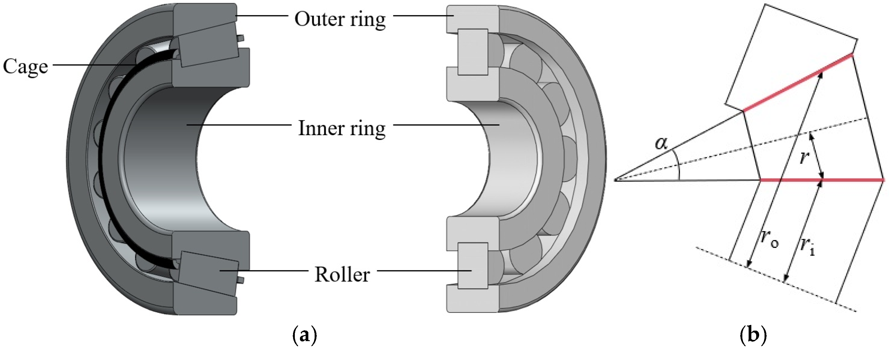
2. Contact Geometry Between Roller and Raceway

As illustrated in Figure 1, a finite line contact bearing comprised an inner ring, an outer ring, rollers, and a cage. The cage served to guide the cylindrical or tapered rollers. In the case of a tapered roller bearing, the axes of rotation for the rollers were inclined with respect to that of the inner ring.

A sectional view of a tapered roller bearing is given by Figure 1b; contact lines are marked in red, the dotted line denotes axis of the roller, the radius of a point on prime line of the roller and axis of the roller is denoted by r, and the cone angle of the roller is denoted by α. The distance between a point on contact line with respect to the inner ring and axis of the bearing is denoted by r_i, and the distance between a point on contact line with respect to the outer ring and axis of the bearing is denoted by r_o. Based on the geometrical parameters of roller, the contact radius at any points on the contact line between the finite line contact roller and the raceway can be obtained, and the expression of contact radius of the roller is as follows:

$$R_{\mathrm{r}}={\displaystyle \frac{a^2}{b}}={\displaystyle \frac{r}{\cos \left(\alpha /2\right)}}$$

(1)

Similarly, the contact radii of the inner ring and the outer ring are R_i = r_i/cos(α/2) and R_o = r_o/cos(α/2), respectively. For a cylindrical roller, α = 0. As shown in Figure 2a, in cross-sections of the roller and the raceway along the normal plane, the parts of roller and the raceway (marked with dotted black lines in the figure) closing to the contact line can be treated as two cylinders, and radii of the cylinders and the contact radii are specified by Equation (1). The vertical distance between profiles of the two cylinders can be further simplified as the vertical distance between the cylinder and a virtual platform (marked with dotted red line in the figure).

The simplified contact geometry between the roller and raceway is given in Figure 2b; the red dashed line depicts the deformed configuration of the equivalent cylinder subjected to the contact load. We denote R as radius of the cylinder, and for the contact between the roller and inner ring, the radius of the cylinder denoting the comprehensive contact radius of the roller and inner ring is R = 1/(1/R_i + 1/R_r). For the contact between the roller and the outer ring, the radius of the cylinder denoting the comprehensive contact radius of the roller and the outer ring is R = 1/(1/R_o − 1/R_r). We denote h as the vertical distance between profile of the cylinder and the platform; the expression of h is as follows:

$$h\left(x\right)=-{\delta }_0+{\displaystyle \frac{x^2}{2R}}+v\left(x\right)$$

(2)

where δ₀ denotes virtual penetration between the roller and the raceway, with a positive value indicating that contact occurs, and v(x) denotes comprehensive deformation between the roller and raceway. Under dry contact conditions, it is assumed the virtual penetration is 0.55 times the mutual approach between the roller and raceway, namely δ₀ = 0.55δ [38].

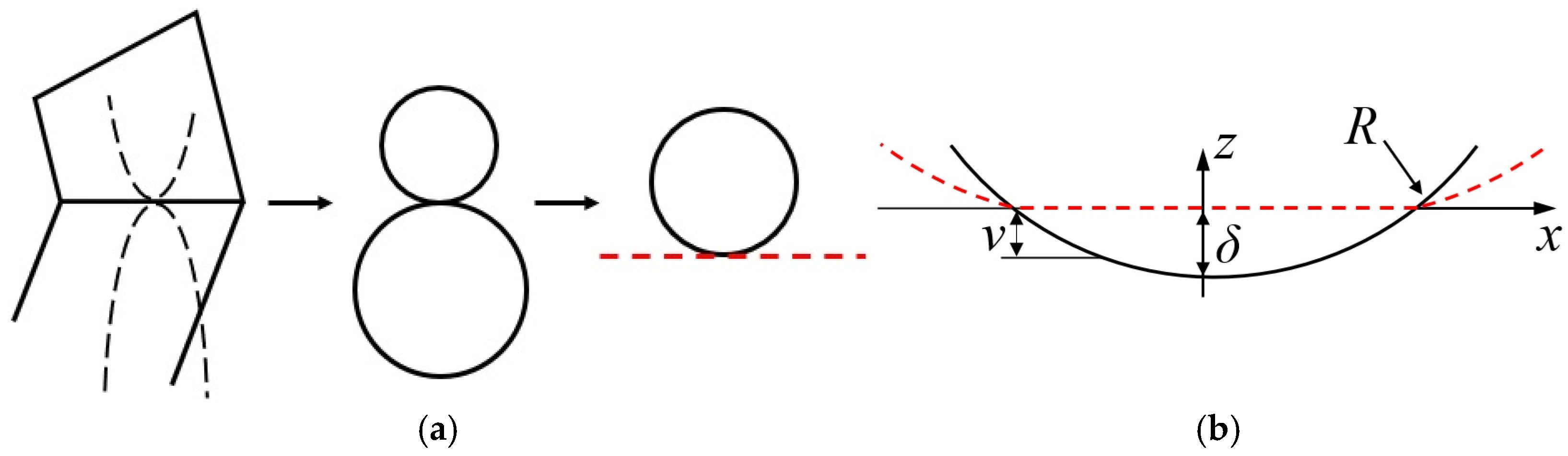
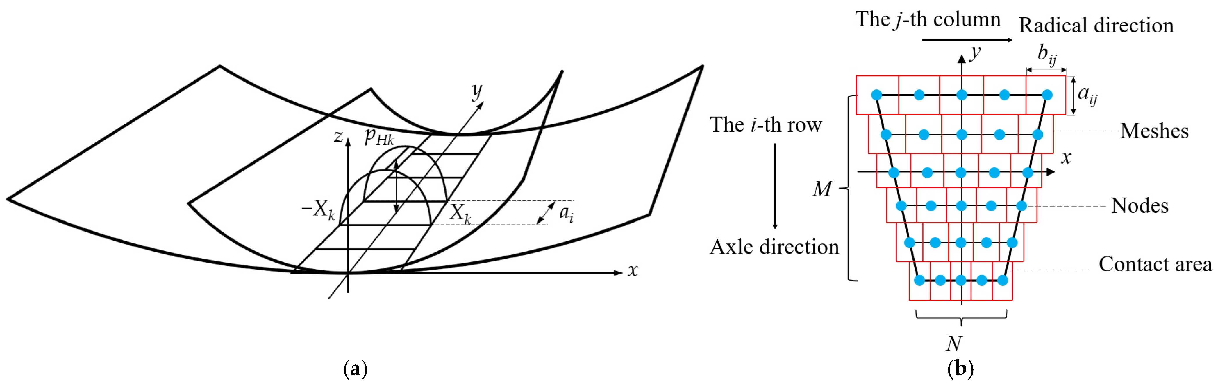
3. Contact Load Calculation Model Based on the Half-Space Theory

Under dry contact conditions, the contact load between the roller and the raceway was typically determined by the deformation of the both surfaces. Based on the half-space theory of Boussinesq [39], the comprehensive contact deformation at a point (x, y) induced by the stress p(x’,y’) is as follows:

$${\displaystyle \frac{1}{\pi E^{\prime }}}{\displaystyle \underset{S}{\iint }\frac{p\left(x^{\prime },y^{\prime }\right)}{\sqrt{{\left(x-x^{\prime }\right)}^2+{\left(y-y^{\prime }\right)}^2}}\mathrm{d}{x}^{\prime }\mathrm{d}{y}^{\prime }}=v\left(x,y\right),{\displaystyle \frac{1}{E^{\prime }}}={\displaystyle \frac{1}{2}}\left({\displaystyle \frac{1-v_1^2}{E_1}}+{\displaystyle \frac{1-v_2^2}{E_2}}\right)$$

(3)

where E’ denotes composite modulus of elasticity of contact surfaces of roller and raceway, E₁ and E₂ denote Young’s modulus of material of roller and raceway, v₁ and v₂ denote Poisson’s ratios of material of roller and raceway. The v(x,y) denotes comprehensive deformation of the contact surface at the point (x, y). By integration, the contact load can be determined through the contact stress. To address the contact stress numerically, it is essential to discretize the contact area into a grid and employ the discretized form of Equation (3) for calculating the contact stress.

To grid the contact area, the roller is sliced into equal-thickness sections along its axle direction, and it is assumed that distribution of the contact stress within each slice remains constant along the axle direction. As shown in Figure 3a, the roller is divided into M equal-thickness slices, and based on the Hertz contact theory, the contact stress within each slice is distributed in a semi-elliptical form along the tangential direction. As shown in Figure 3b, to quantitatively assess the contact stress within each slice, the stress within each slice is represented by stress values of N equally spaced nodes. Based on this grid division method, Equation (3) is discretized as follows:

$${\displaystyle \frac{1}{\pi E^{\prime }}}{\displaystyle \sum _{i=1}^M{\displaystyle \sum _{j=1}^N{K}_{kl}^{ij}\cdot }}{p}_{ij}=v_{kl}$$

(4)

where K^ij_kl denotes the influence coefficient of the stress exerted on the node of the i-th row and the j-th column, with respect to the deformation of the node situated at the node of the k-th row and the l-th column. Similarly, p_ij denotes the stress exerted on the node of the i-th row and the j-th column, and v_kl denotes the comprehensive deformation of the node of the k-th row and the l-th column. Expression of the influence coefficient K^ij_kl is as follows:

$$\begin{array}{l}{K}_{kl}^{ij}=I\left(x_{kl}^{ij}+{\displaystyle \frac{b_{ij}}{2}},y_{kl}^{ij}+{\displaystyle \frac{a_{ij}}{2}}\right)-I\left(x_{kl}^{ij}+{\displaystyle \frac{b_{ij}}{2}},y_{kl}^{ij}-{\displaystyle \frac{a_{ij}}{2}}\right)-I\left(x_{kl}^{ij}-{\displaystyle \frac{b_{ij}}{2}},y_{kl}^{ij}+{\displaystyle \frac{a_{ij}}{2}}\right)+I\left(x_{kl}^{ij}-{\displaystyle \frac{b_{ij}}{2}},y_{kl}^{ij}-{\displaystyle \frac{a_{ij}}{2}}\right)\\ I\left(x,y\right)=x\ln \left(y+\sqrt{x^2+y^2}\right)+y\ln \left(x+\sqrt{x^2+y^2}\right),\left\{\begin{array}{c}{x}_{kl}^{ij}=\left|x_{ij}-x_{kl}\right|\\ y_{kl}^{ij}=\left|y_{ij}-y_{kl}\right|\end{array}\right.\end{array}$$

(5)

where a_ij and b_ij denote length and width of the mesh located at the i-th row and the j-th column, respectively. As the slices are of equal thickness, and nodes within a slice are equally spaced, following the Hertz theory, the length and width of the meshes are simplified as follows:

$$a_i=a_{ij}=L/\left(M-1\right),\begin{array}{cc}{b}_i=\sqrt{{\displaystyle \frac{8w_i{R}_i}{a_i\pi E^{\prime }}}},& b_{ij}=\end{array}{\displaystyle \frac{2}{N-1}}{b}_i$$

(6)

where w_i denotes the contact load applied on the i-th roller slice; R_i denotes the comprehensive contact radius of the i-th roller slice; b_i denotes the contact half-width of the i-th roller slice; and L denotes the length of the roller. Assuming that the stress distribution of roller slices follow Hertzian theory, the correlation between the center deformation of the roller slice and the stress at the roller slice center can be expressed in matrix form as follows.

$$C\cdot W=V$$

(7)

where C denotes the flexibility coefficient matrix, W denotes a vector formed by contact loads of nodes on the contact line, and V denotes the vector formed by deformations of nodes on the contact line. The expression of the matrix C is as follows:

$$C=\left[\begin{array}{ccc}{c}_{1,1}& \cdots & c_{1,M}\\ ⋮& \begin{array}{ccc}\ddots & & \\ & c_{k,i}& \\ & & \ddots \end{array}& ⋮\\ c_{M,1}& \cdots & c_{M,M}\end{array}\right]$$

(8)

where c_k,i represents the flexibility coefficient of the node, indicating the relationship between the central deformation of the k-th roller and the load applied at the node located at i-th row and j-th column. Expression of the coefficient c is as follows:

$$c_{k,i}={\displaystyle \frac{2}{{\pi }^2{E}^{\prime }{a}_x{b}_x}}{\displaystyle \sum _{j=-(N-1)/2}^{\left(N-1\right)/2}\left(K_{k-\frac{M+1}{2},0}^{i-\frac{M+1}{2},j}\sqrt{1-{\left(\frac{2j}{N-1}\right)}^2}\right)}$$

(9)

As width of a mesh, namely b_ij, which is derived from half-width of contact area of a roller slice, has a significant impact on calculating results of the contact load, and the half-width relates to the undetermined contact load, an iterative procedure is employed to approximate the solutions of the full half-space theory specified by Equation (3). In the iteration, b_i is repeatedly calculated through Equation (6). The pseudocode of the iterative calculation procedure is shown in Algorithm 1.

Algorithm 1 The Contact Load Calculating Model Based on the Half-Space Theory
Require:  Parameters: Radius of roller R; Contact line length L; Mutual approach δ; Mesh  numbers M, N; Composite modulus of elasticity E  Tolerance: e Ensure:  Half width of contact area for each roller slice bi
1: //Initialize
2: $b_i\leftarrow \sqrt{2R_i{\delta }_i}$	▷ Contact width of the i-th roller slice
3: $a_i\leftarrow L/N$	▷ Length of mesh of the i-th roller slice
4: $e_0\leftarrow \mathrm{e}+1$	▷ Current difference, initialized to e + 1
5: $b_{0i}\leftarrow b_i$	▷ Initial contact width
6: while $e_0>e$do
7:  // Influence coefficient matrix construction
8:  Matrix $\leftarrow$ matrix_construction (M, N, ai, bi)
9:  // Contact load update
10:  W $\leftarrow$ Matrix-1 × δ
11:  Wi $\leftarrow$W[i]	▷ Extract the i-th contact load
12:  // Contact width update
13:  $b_i\leftarrow \sqrt{8W_{i}R/\left(a_i\pi E\right)}$
14:  //Calculate error
15:  $e_0 \leftarrow \sum \left|b_{0i}/b_i-1\right|$
16:  $b_{0i}\leftarrow b_i$
17: end while
18: return Wi

Since the deformation vector V in Equation (7) is formed by the deformation of each roller slice, the effects of surface roughness on real contact mechanics can be considered. Assuming that the surface roughness between the roller and the raceway is R_a, the comprehensive deformation of each roller slice is the result of the superposition of mutual approach and surface roughness effects. With the surface roughness of 0.001 mm, and the mutual approach of 0.01 mm, a diagram of the contact load acting on each roller slice of a steel roller with a radius of 10 mm and a length of 40 mm calculated by the proposed model is shown in Figure 4.

As shown in Figure 4, when the effect of surface roughness was considered, the comprehensive deformations of roller slices became inconsistent, and the corresponding contact loads of each roller slice also fluctuated. The results indicate that the proposed model could effectively reflect the influence of surface roughness effect on the contact loads.

4. Fast Method for the Contact Load Calculation Model

The iterative progress for determining contact width of each roller slice is time consuming, which seriously affects the computational efficiency of calculating the contact loads by using the half-space theory. As the distances between the nodes located in different roller slices are much greater than that in the same roller slice, the influence of the inter-slice contact stress on deformation of local roller slice can be ignored, and the calculation of the contact load turns to a plane strain issue. Under the plane strain issue, the contact half-width calculation conducted in two-dimensional grids is transferred to be conducted in one-dimensional grids, which is more efficient. When the influences of the inter-slice contact stress on the deformations are ignored, the formula for calculating the deformations under contact stresses is as follows:

$$v\left(x\right)=-{\displaystyle \frac{2}{\pi E^{\prime }}}{\displaystyle {\int }_{s_1}^{s_2}p\left(s\right)\ln {\left(s-x\right)}^2\mathrm{d}s}$$

(10)

Based on Equation (10), under the Hertzian stress distribution theory, the relationship between the central deformation of roller and stresses applied on the contact area of the roller is as follows:

$$v\left(0\right)=-{\displaystyle \frac{8p_{0}b}{\pi E^{\prime }}}{\displaystyle {\int }_0^1\ln \left(b\cdot X\right)\sqrt{1-X^2}\mathrm{d}X}$$

(11)

According to Equation (11), after performing the integral calculation, when both the materials of roller and raceway are steel, a nonlinear equation relating the contact bandwidth b to the deformation v can be derived as follows:

$$v\left(0\right)=-{\displaystyle \frac{b^2}{2R}}\ln b+{\displaystyle \frac{b^2}{4R}}\left(1+\ln 4\right)$$

(12)

The half-width of contact area of the i-th roller slice can be solved according to Equation (12) through the Newton–Rapson algorithm, and then the influence matrix can be constructed according to Equation (8); the contact load is solved through Equation (7). A comparison of deformations calculated by the fast method and the iterative procedure of the cylindrical roller specified in

Table 1. Geometrical parameters of roller.

	Cylincal Roller	Tapered Roller
Length of roller	11.5 mm	15.5 mm
Diameter of roller at the small end	8.5 mm	6.68 mm
Diameter of roller at the big end	8.5 mm	10.85 mm
Cone angle of roller	0°	7.64°

is given by Figure 5. As shown in the figure, the contact area obtained by the fast algorithm was flatter than that obtained by the full half-space theory.

When the roller slice is not in contact with the raceway, contact half-width of the roller slice is 0, and influence coefficients relating to the roller slice is also 0. So, for the roller slices that are no longer in contact with the raceway, the influence coefficients for these slices are excluded from the matrix, and the deformations are therefore not taken into consideration when calculating contact loads through Equation (8). To compare the differences in contact force calculated by various methods as well as the computational efficiency of the methods, cylindrical rollers with diameters varying in 5-mm increments, ranging from 5 mm to 25 mm, are utilized for the comparison, and the ratio of length to diameter of the roller was set to 2:1. The contact area was grided into a mesh measuring M by N, where M = 51 and N = 27. The tolerance used by the iterative procedure was set to 0.05. The above calculations were performed using an in-house computer code developed in MATLAB^® R2021a with a laptop using processor AMD Ryzen 7 5800H @ 3.20 GHz. The deformations of the rollers varied from 0.001 mm to 0.009 mm, contact loads obtained by various methods are presented by Figure 6a, and the time taken to complete the load calculation with respect to a roller diameter of different methods are presented by Figure 6b. In Figure 6a, the stars represent the loads obtained by the fast method, the boxes represent the loads obtained by the iterative procedure applying full-order model of half-space theory, and the colors between the lines indicate the differences in loads obtained by various methods for rollers with different radii. As shown in Figure 6a, the loads obtained by the fast method are less than those obtained by the full-order model. The calculation errors of the fast method relative to the full-order model are presented in Figure 6a with black triangles. The results indicate that the error decreased with increasing deformation, which implies that the error will decrease with increasing applied contact load. As shown in Figure 6b, the time taken by the fast method is much less than the time spent by the iterative procedure, and the fast method reduces the calculation time by approximately 77%.

5. Contact Load Calculation Under Lubricated Condition

The fast method can be used to calculate contact load between roller and raceway under the lubricated condition when deformations between the roller and the raceway are determined. Geometric implications of the contact are shown in Figure 7, where h₀ denotes the central film thickness at the contact center and v₀ denotes the deformation at the contact center.

For the i-th slice of the roller, a geometrical relation between the parameters shown in Figure 7 can be established and is given by Equation (13). The central film thickness between the i-th roller slice and the raceway is predicted by Dowson–Higginson formula [36], which is given by Equation (14).

$$h_{0i}-{\delta }_{0i}-v_{0i}=0$$

(13)

$$h_{0,i}=3.533{\displaystyle \frac{{\left[L/\left(M-1\right)\right]}^{0.13}{R}_i^{0.43}{\alpha }^{0.54}{\left({\eta }_{0}u\right)}^{0.7}}{{E^{\prime }}^{0.03}{w}_i^{0.13}}}$$

(14)

$$w_i={\displaystyle \frac{b_i^{2}L\pi E^{\prime }}{8R_i\left(M-1\right)}}$$

(15)

where u denotes the relative speed between the roller and the raceway, α denotes the adhesive pressure coefficient, and η₀ denotes the viscosity of lubricant under zero pressure. Under Hertzian assumptions, the relationship between contact width of roller slice and contact load applied on roller slice is given by Equation (15). Substituting the expressions specified in Equations (12), (14), and (15) into Equation (13), a formula relating to contact widths of roller slices under the lubricated condition can be established and is given by Equation (16).

$$f\left(b_i\right)=4.6296{\displaystyle \frac{R_i^{0.56}{\alpha }^{0.54}{\left({\eta }_{0}u\right)}^{0.7}}{{E^{\prime }}^{0.16}{\left(b_i^2\pi \right)}^{0.13}}}-{\delta }_i+{\displaystyle \frac{b_i^2}{2R}}\ln b-{\displaystyle \frac{b_i^2}{4R}}\left(1+\ln 4\right)$$

(16)

where the term δ_i denotes the mutual approach of the i-th roller slice. When b_i has been solved from the nonlinear Equation (16), the contact load applied on roller slices can be directly obtained through the Equation (15). In particular, after the contact width has been calculated under lubrication conditions, the contact load cannot be determined using Equation (7). Instead, the contact load applied on roller slice was calculated separately employing Equation (15), because the contact load derived directly from the contact width corresponded to the film thickness. If Equation (7) is used to solve for the contact load, the relationship between the film thickness and the contact load would be disrupted.

6. Comparison of the Proposed Model with Other Models

The difference between the proposed model and other models is demonstrated by comparing the contact loads per length calculated by this model with those calculated by alternative models under varying deformation conditions. The geometrical parameters of the roller and the raceway, as well as the models introduced by reference [15], and the contact loads per length obtained by the different models without energy dissipation relative to the contact deformation depths are given by Figure 8. As shown in Figure 8, the contact loads per length obtained by the different models exhibit significant differences, and the results obtained by the proposed model are among the results obtained by Liu and Dubowsky–Freudenstein, which are closer to that of Dubowsky–Freudenstein’s.

To further compare the stress obtained by the proposed model and the stress obtained by FEA, two rollers were chosen. One of the chosen rollers was cylindrical, and the other was tapered. The cylindrical roller belonged to the bearing 352,210, and the tapered roller belonged to the bearing NH2210. The geometrical parameters of the rollers are listed in Table 1.

The elasticity modulus and Poisson’s ratio of materials of the roller and the raceway are set to 206 GPa and 0.3, respectively. As shown in Figure 9, the rollers were constrained to make contact with cuboids whose lengths matched those of the prime lines of the rollers. The surface nodes on the upper halves of the rollers were constrained to move at a specified distance vertically as part of the mutual approach, while the nodes on the bottom surfaces of the cuboids were fully fixed. When surface nodes of the upper half of the rollers were constrained to move 0.01 mm, the cloud maps of stress distributions and displacements of nodes, as well as displacements of nodes located on the contact lines are shown in Figure 10.

As shown in Figure 10b,d, the displacement of surface nodes of the upper half of the rollers is −0.01 mm, and as shown in Figure 10e, the node displacements on the contact line of the cylindrical roller is about −4.5 × 10⁻³ mm, while the node displacements on the contact line of the tapered roller varied from −5 × 10⁻³ mm to −3.5 × 10⁻³ mm. Taking the average displacements of the nodes on the roller contact lines as the representative displacements of the roller at their contact lines, the deformations of the rollers at the contact lines were regarded as the differences between the constrained displacements and the displacements of the nodes on the roller contact lines, which were 5.5 × 10⁻³ mm and 5.75 × 10⁻³ mm, respectively. To implement the proposed fast method, the contact area was grided into a mesh measuring M by N. To be consistent with FEA, M was set to 61, and N was set to 15. Incorporating geometric parameters of rollers and the deformations into the proposed model, the stresses of the nodes on the contact line obtained by the fast method and those obtained by FEA are shown in Figure 11.

As shown in Figure 11a, the stresses of nodes on the contact line of the cylindrical roller are symmetrical, and the stress intensities at ends of the contact line are significantly higher than those near the middle region. As shown in Figure 11b, the stresses of the nodes along the contact line of the tapered roller are asymmetrical. The stress intensities at the ends of the contact line are significantly higher than those near the middle region, and the stresses closer to the smaller-diameter end of the roller are higher than those closer to the larger-diameter end. The stresses obtained by FEA and the proposed model are close, and the localized error of the stresses obtained by the proposed model relative to that obtained by FEA were evaluated and are shown in Figure 12.

As shown in Figure 12, the localized errors of the stress near the middle region and the ends of the contact line for the cylindrical roller are greater, while the localized error for the tapered roller near the larger-diameter end was much more significant. In general, the localized error of the cylindrical roller was higher than that of the tapered roller. The mean error of stress calculation of the cylindrical roller was about 20%, while that of the tapered roller was about 6%. The discrepancies between the stresses obtained by FEA and those obtained by the model arise because the stress distribution observed in FEA do not fully conform to Hertzian theory, and the rollers exhibit longitudinal deformations in FEA.

To compare the total contact load obtained by FEA and the proposed model, five groups of mutual approaches were selected as movement constraints for the rollers, which were 0.005 mm, 0.0075 mm, 0.01 mm, 0.0125 mm, and 0.015 mm, separately. The total contact loads obtained by different methods are presented in Figure 13, as well as the error of loads obtained by the proposed model relative to those obtained by FEA.

As shown in Figure 13, the total contact loads increase with increasing in mutual approaches. The differences between the total contact loads of the cylindrical roller obtained by different methods are small, while the differences between the total contact loads of the tapered roller obtained by different methods are relatively large. With the increase in deformation, the differences between the total contact loads of the tapered roller become more pronounced. The average error of the obtained loads with respect to the cylindrical roller is about 2%, and the average error of the obtained loads with respect to the tapered roller is about 17%. As a result, the proposed model is more suitable for the contact load calculation of a cylindrical roller and improper for the contact load calculation of a tapered roller with relatively large mutual approaches.

7. Dynamic Simulation and Experimental Validation

An experimental test was conducted to verify the results derived from the bearing dynamic models utilizing the proposed model. In the constructed bearing dynamic model, both the inner ring and the outer ring were defined with six rigid body degrees of freedom, while the rollers were defined with four degrees of freedom, and the cage was defined with one degree of freedom. The four degrees of freedom of the roller were defined as the translational movement along the y-axis and z-axis, as well as the rotational motion around the y-axis and x-axis. The angular displacement of the roller around the x-axis, denoted as ϕ_r, was employed to characterize the roller’s incline with respect to the raceway. The cage was defined as rotating around the axis of the inner ring. As illustrated in Figure 14, frames with respect to the components of the bearing model were employed to delineate the contact profile between the roller and the raceway. The origin of the inner ring coordinate frame was situated at the center of mass of the inner ring, and the coordinate axes were denoted as x_i, y_i, and z_i, with the y_i-axis aligned along the inner ring axis, while the x_i and z_i axes lied in the radial direction of the inner ring. The number of roller coordinate frames equaled the number of rollers, and the origins of all roller coordinate frames were situated at the center of the inner ring. Additionally, the y-axis (referred to as y_rk for the y-axis of the k-th roller) in all roller coordinate frames aligned with the y_i-axis, while the z-axis (referred to as z_rk for the z-axis of the k-th roller) in each roller coordinate frame pointed towards the angle where the center of the k-th roller was positioned. The origin of the outer ring coordinate frame was located at the center of mass of the outer ring, and the coordinate axes were denoted as x_o, y_o, and z_o. The mutual approach between roller and raceway was calculated according to coordinates of inner ring, outer ring, and rollers. The bearing used for dynamic simulation and experiment was a 352,210 double-row tapered roller bearing. The inner ring of the bearing was installed on a shaft, which was fixed by deep groove ball bearings 6209. Geometrical parameters of the bearing, as well as the surface roughness and number of the nodes, are listed in

Table 2. Parameters of bearing 352210.

Parameter	Value
Elasticity modulus of materials	206 GPa
Poisson’s ratio of materials	0.3
Length of roller	15.68 mm
Diameter of roller at the small end	6.68 mm
Diameter of roller at the big end	10.85 mm
Diameter of outer ring at the small end	70.0 mm
Diameter of outer ring at the big end	82.0 mm
Diameter of inner ring at the small end	56.66 mm
Diameter of inner ring at the big end	60.90 mm
Cone angle of outer ring	22.3°
Cone angle of inner ring	7°
Viscosity	0.1 Pa·s
Number of nodes	31 (M) × 51 (N)
Surface roughness	0.001 mm

. The degrees of freedom of the bearing model are listed in

Table 3. Degrees of freedom of the bearing model.

	x	y	z	ϕ	β	ψ
Inner ring	xi	yi	zi	ϕi	βi	ψi
Outer ring	xo	yo	zo	ϕo	βo	ψo
Roller	-----	yr	zr	ϕr	βr	-----
Cage	-----	-----	-----	-----	βc	-----

.

In Table 3, ϕ, β, and ψ denote the rotations of the respective components around the x-axis, y-axis, and z-axis, respectively, ‘----’ denotes the vanishing of the corresponding degree of freedom. The tangential forces acting on rollers that drag the rollers’ rotating and spinning were simplified to forces related to contact loads and drag coefficients [40]. When the load applied on a roller diminished to zero, the tangential force vanished entirely, then the rotation of the roller was driven by the cage. As shown in Figure 15, interaction between rollers and cage was calculated according to mutual approach between the pocket holes and rollers using Dubowsky–Freudenstein’s method.

As shown in Figure 15, the length of the pocket hole is denoted by l_c, and the initial clearance between the edges of the pocket hole and roller is denoted by ∆u. The mutual approach between roller and cage is obtained by the following formula:

$${\delta }_{\mathrm{c}}=D\cdot \left({\beta }_{\mathrm{r}}-{\beta }_{\mathrm{c}}\right)/2-d/2-\mathsf{\Delta }u$$

(17)

The dynamic simulation and the experiment were conducted under different speeds, applied loads, and contact conditions. The physical drawing of the bearing test bench and the cross-sectional view of the test bench are presented in Figure 16. As illustrated in Figure 16b, utilizing the lever principle, a fine-threaded bolt is affixed to one side of the bearing housing for applying load to the bearing, while a load sensor is positioned on the opposite side of the bearing housing to capture the signal of the applied load. Vertical acceleration signals of the bearing housing under the various contact conditions outlined in

Table 4. Central frequencies under different rotating speeds.

No.	Contact Condition	Rotational Speed	Applied Load
1	Lubricated	600 RPM	1000 N
2	Lubricated	1200 RPM	1000 N
3	Dry	600 RPM	1000 N
4	Dry	1200 RPM	1000 N

were calculated through the bearing dynamic model, and the corresponding signals were acquired through an acceleration sensor mounted on the bearing housing. The signal was acquired using an IMC data acquisition device with a sampling frequency of 10⁵ Hz, and a load sensor was installed to capture the signal of the applied load. Under the lubricated condition, the bearing was lubricated by grease.

The signals obtained through the dynamic simulations and the experiments are presented in Figure 17. As illustrated in the figure, the acceleration signals of the bearing acquired through experimentation demonstrate significantly higher amplitudes as the rotational speed increases from 600 RPM to 1200 RPM. Moreover, the amplitudes of the experimental acceleration signals obtained under dry conditions are greater than those obtained under lubricated conditions at the same rotational speeds. The Root-Mean-Square (RMS) values of the signals calculated by the dynamic simulation and acquired through the experiments are listed in

Table 5. RMS values of signals.

No.	Condition	Speed (RPM)	Simulation (m/s2)	Epxeriment (m/s2)	Error (%)
1	Lubricated	600	2.442	1.767	38.2
2	Lubricated	1200	5.681	4.057	40.0
3	Dry	600	3.447	2.734	26.1
4	Dry	1200	10.121	10.714	5.5

. The results presented in the table demonstrate that the amplitudes of the simulated signals are closely aligned with those of the experimental signals. However, the maximum error between the RMS values of the simulated and experimental signals was 40%. The discrepancies in the RMS values might stem from the fact that the contact deformations approximated by the mutual approaches in the simulations differed from the actual deformations, thereby causing a deviation between the simulated contact forces and the actual contact forces. Consequently, the amplitudes of the acceleration signals obtained through simulations and the measured signals were inconsistent. Compared with the dry contact conditions, the error between RMS values of the signals obtained under the lubricated conditions are more pronounced, which might be attributed to the fact that the damping effect of lubrication was not adequately accounted for in the model.

The results of the signal spectrum analysis are presented in Figure 18. As shown in Figure 18, under dry contact conditions, the spectrum amplitudes of the observed simulated acceleration signals are higher than those under lubrication conditions. Meanwhile, the frequency ranges associated with the regions of higher spectral densities under dry contact conditions are higher than those associated with the regions of higher spectral densities under lubricated contact conditions. These spectral distributions are consistent with the distributions of the experimental signal spectrum presented in Figure 18 under different experimental conditions. This phenomenon can be attributed to the fact that, under dry contact conditions, the contact stiffness between rollers and raceways calculated by the proposed model was greater than that under lubricated conditions, thereby causing the frequency of the acceleration response signal under dry contact conditions to be higher than that under lubricated conditions. The central frequencies of the signal spectra are presented in

Table 6. Central frequencies of spectrums of signals.

No.	Condition	Speed (RPM)	Simulation (Hz)	Epxeriment (Hz)	Error (%)
1	Lubricated	600	3450	3075	12.2
2	Lubricated	1200	3662	3756	2.3
3	Dry	600	4843	5948	18.6
4	Dry	1200	5061	6792	25.5

. The results presented in the table indicate that the frequencies of the signals obtained under lubricated conditions are lower than those obtained under dry contact conditions. Moreover, the discrepancies among the central frequencies of the spectra under lubricated conditions are relatively small compared to those under dry contact conditions.

In general, the contact stiffness between the roller and raceway predicted by the proposed model was relatively reliable. However, when directly applying the model to the bearing, the dynamic model might lead to an error of contact loads. Therefore, in future studies, the damping effect between contacts will be considered to further enhance the proposed model. Additionally, the conversion relationship between deformation and mutual approach will be investigated in more detail, and the criteria for using the proposed model under lubricated conditions will be further evaluated.

8. Conclusions

In order to fulfill the demands of a dynamic bearing simulation, a model is developed in this study to predict contact load for finite line contact rollers of bearings based on the half-space theory. A fast method was proposed to enhance the computational efficiency of the constructed model, and the proposed fast method was applied to EHL problem based on the Dowson–Higginson formula. Simulations were conducted to verify applicability of the proposed model. The outcomes of this study could be summarized as follows:

(1)

An algorithm for calculating contact load of finite line contact roller based on the half-space theory was developed, in which the iterative procedure was used to determine the contact half-width of each roller slice, and the influence coefficient matrix was constructed to solve for the contact load of each roller slice.

(2)

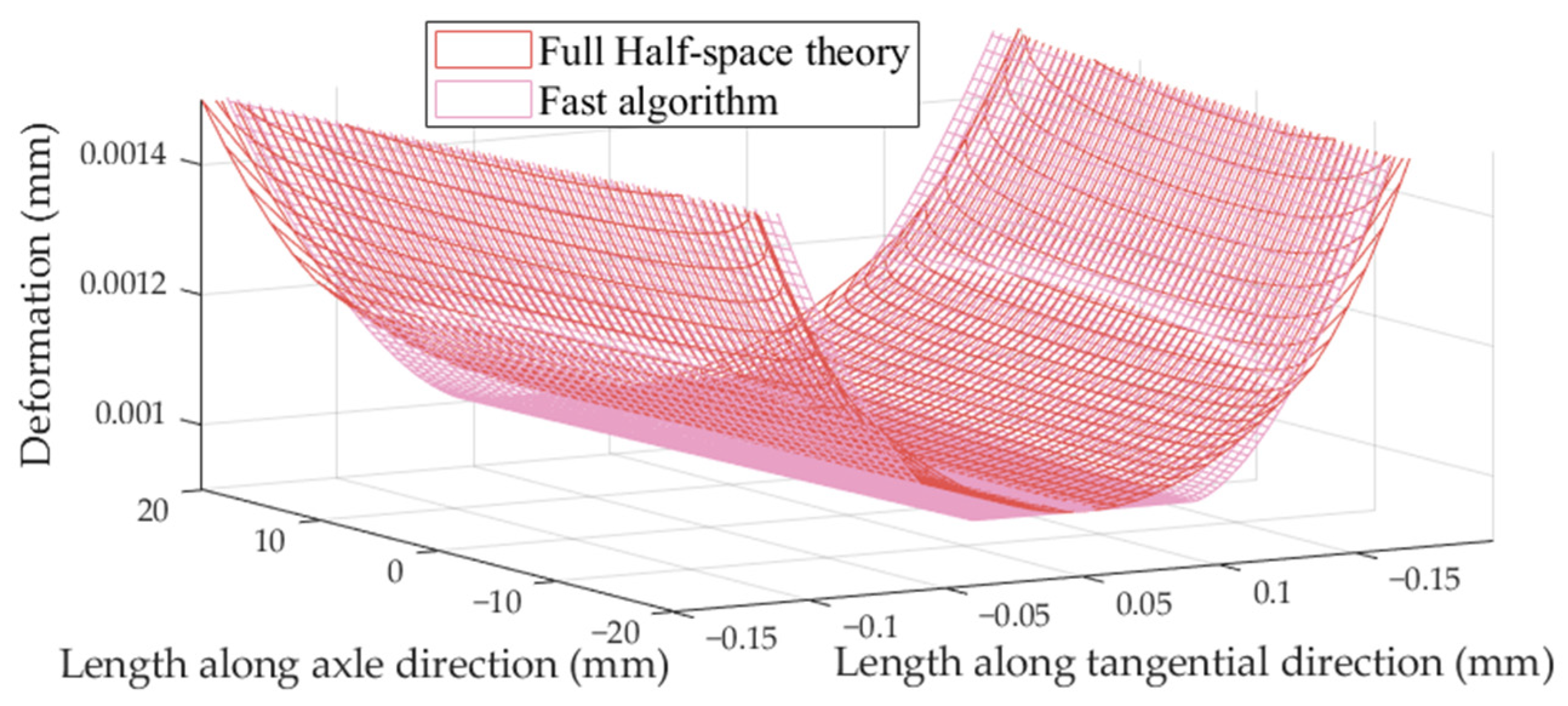
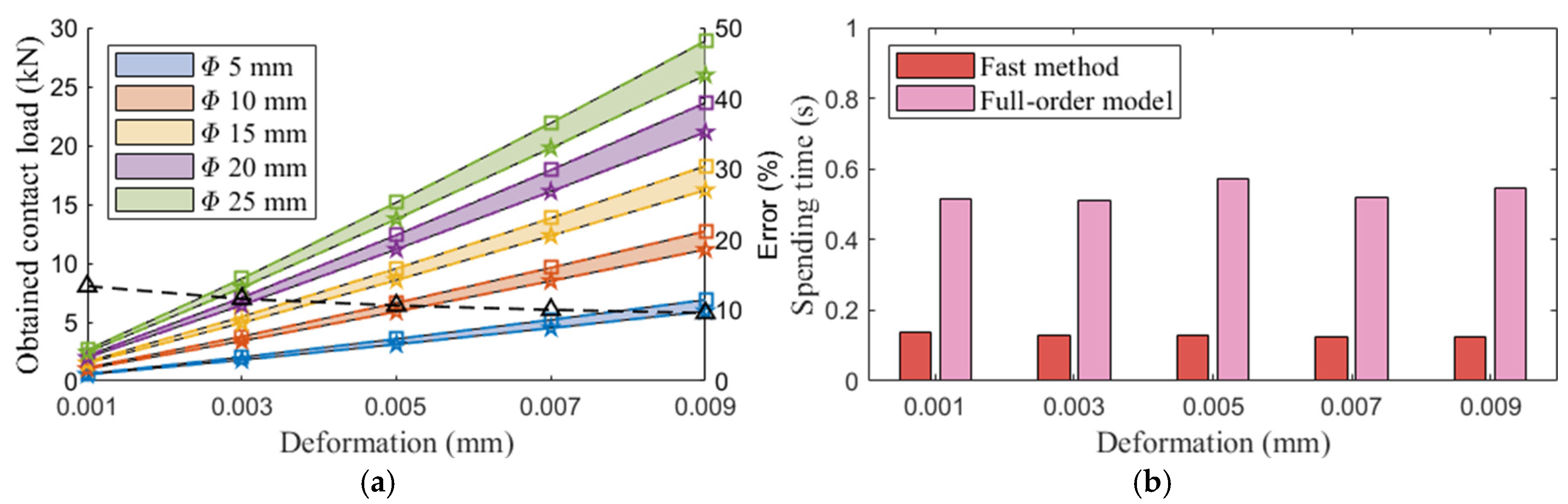
A fast algorithm for calculating rolling contact load was developed, and the disparity in contact load calculation results between the full half-space theory and the fast method were compared. The results indicated that the errors of the fast method relative to the full-order model decreased with increasing the contact load applied on the roller, and the fast method reduced the calculation time by approximately 77% compared to the iterative procedure.

(3)

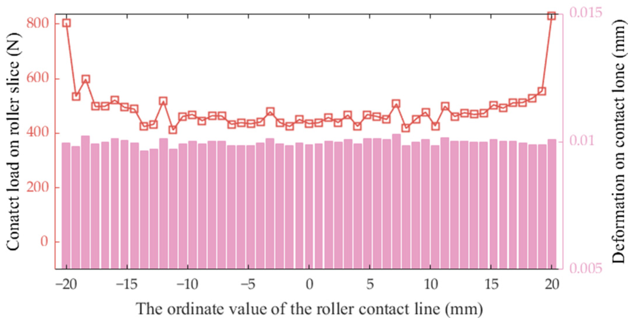
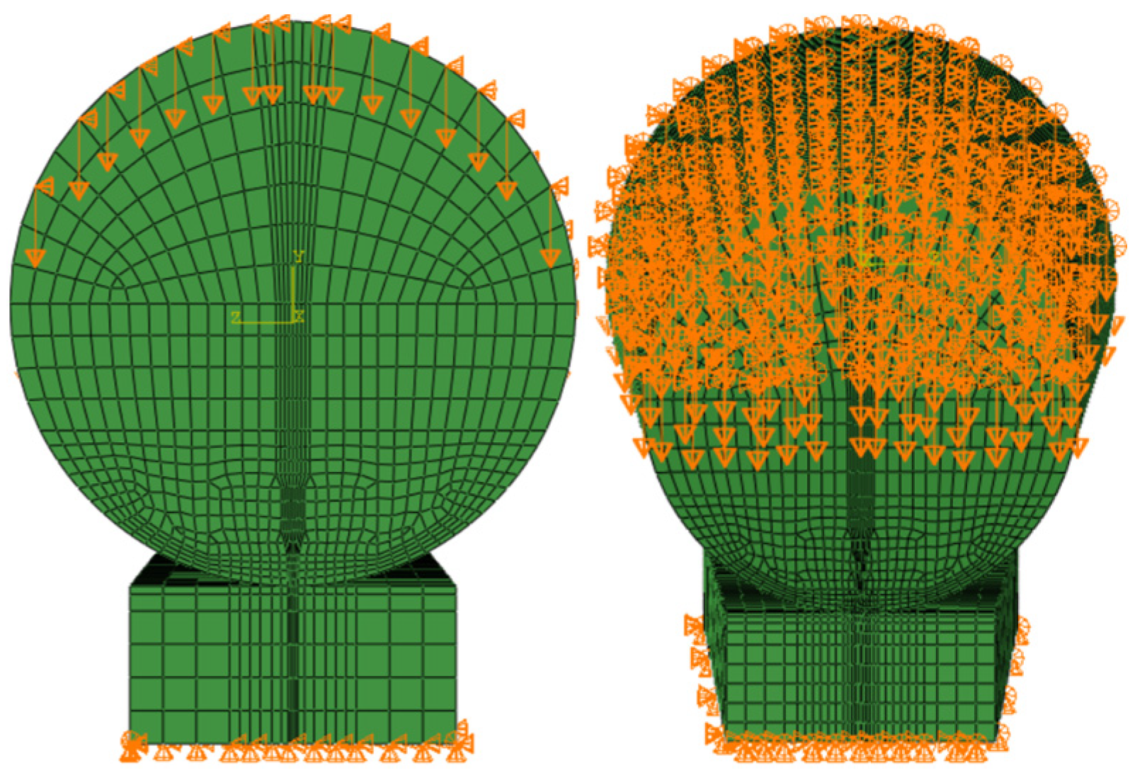
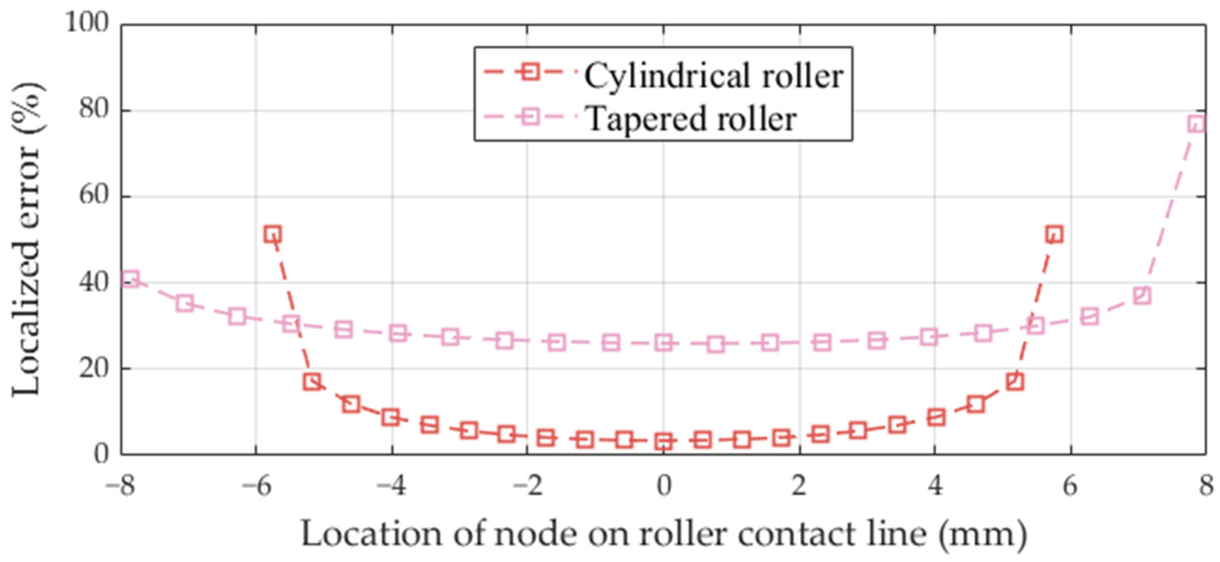
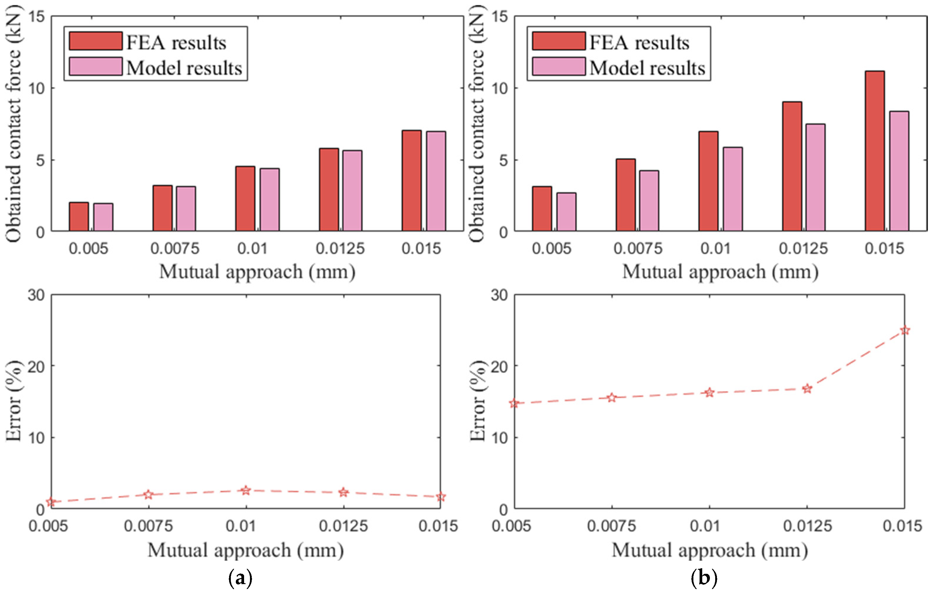
A cylindrical roller and a tapered roller were utilized to compare stresses and contact loads obtained by the proposed model and FEA. The stress calculation results indicated that the localized errors of the stress near the ends of the rollers were much greater than those near the middle region, and the errors for the tapered roller were more significant compared with those for the cylindrical roller. Nevertheless, the differences between the contact loads obtained by the proposed model and FEA for the cylindrical roller were smaller than those for the tapered roller.

(4)

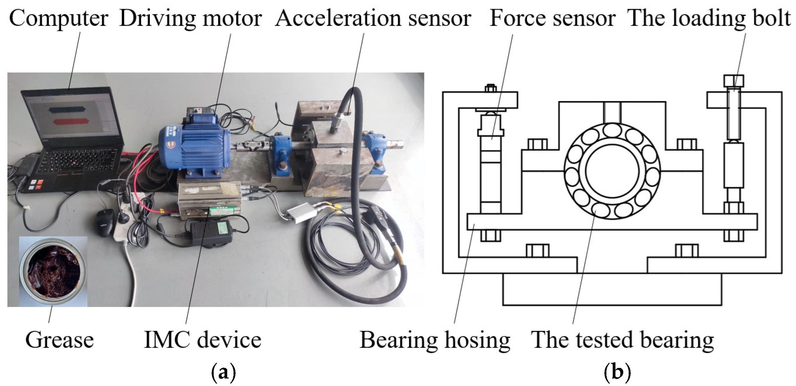
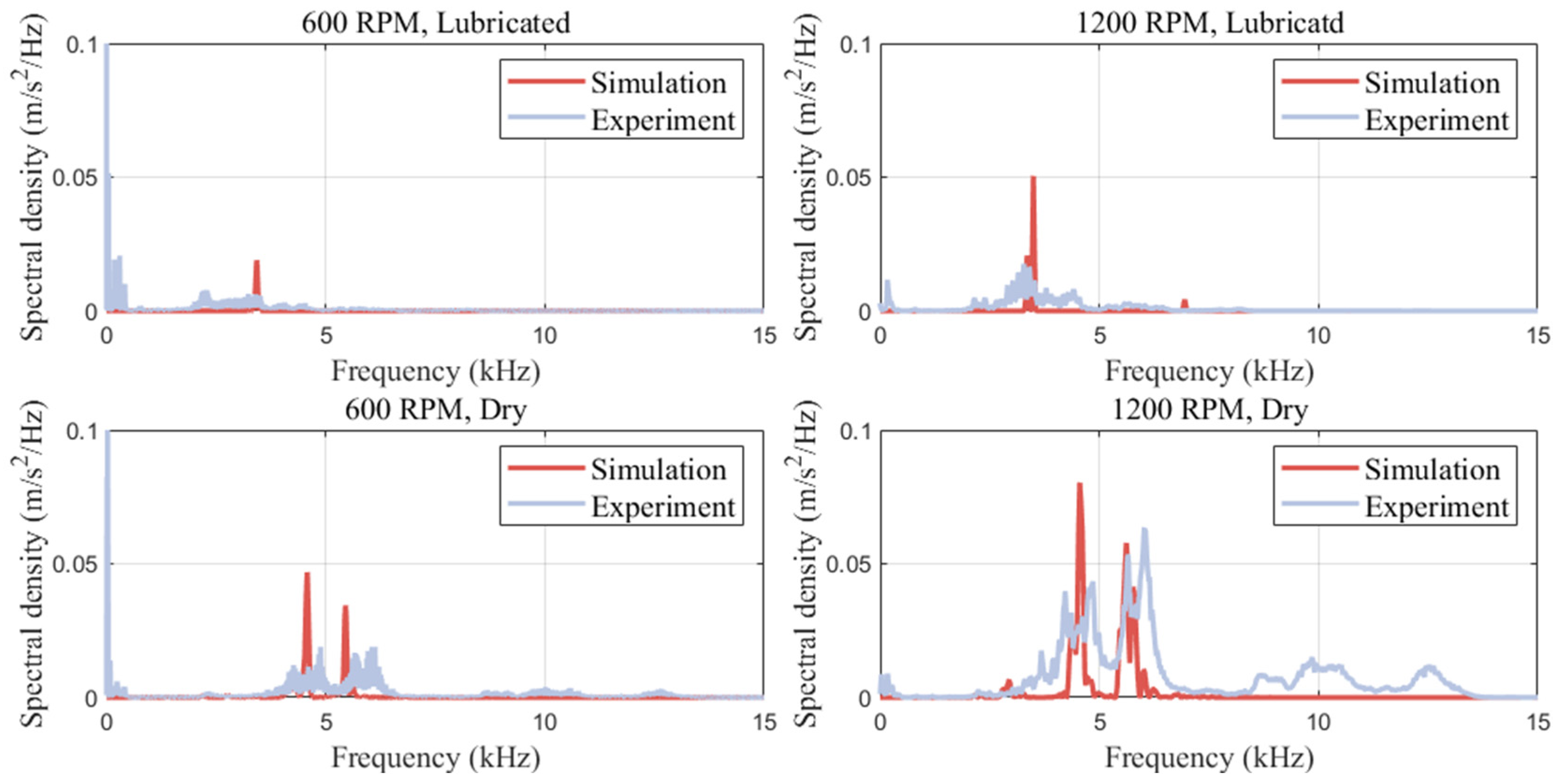
Dynamic simulations and experiments were conducted to verify applicability of the proposed model, and the results indicated that the contact stiffness between the roller and raceway predicted by the proposed model was higher under the dry contact conditions than that under the lubricated conditions.

The model proposed in this study can be utilized to accurately calculate the contact loads between the roller and the raceway for dynamic simulations of finite line contact roller bearings, while considering surface roughness and the localized interaction between the deformation and the contact load. However, the discrepancies between the results obtained in simulations and experiments indicate that the model needs to be further enhanced. Therefore, time-varying parameters will be incorporated into the model in future studies to reflect the damping effect between the contacts, and the conversion relationship between the deformation and the mutual approach will be examined in greater detail.

References

1. Moazen Ahmadi, A.; Petersen, D.; Howard, C. A nonlinear dynamic vibration model of defective bearings—The importance of modelling the finite size of rolling elements. Mech. Syst. Signal Process. 2015, 52–53, 309–326. [Google Scholar] [CrossRef]
2. Yan, P.; Yan, C.; Wang, K.; Wang, F.; Wu, L. 5-DOF Dynamic Modeling of Rolling Bearing with Local Defect considering Comprehensive Stiffness under Isothermal Elastohydrodynamic Lubrication. Shock Vib. 2020, 2020, 1–15. [Google Scholar] [CrossRef]
3. Cui, L.; Zhang, Y.; Zhang, F.; Zhang, J.; Lee, S. Vibration response mechanism of faulty outer race rolling element bearings for quantitative analysis. J. Sound Vib. 2016, 364, 67–76. [Google Scholar] [CrossRef]
4. Petersen, D.; Howard, C.; Prime, Z. Varying stiffness and load distributions in defective ball bearings: Analytical formulation and application to defect size estimation. J. Sound Vib. 2015, 337, 284–300. [Google Scholar] [CrossRef]
5. Kabus, S.; Hansen, M.R.; Mouritsen, O. A new quasi-static cylindrical roller bearing model to accurately consider non-hertzian contact pressure in time domain simulations. J. Tribol. 2012, 134, 041401. [Google Scholar] [CrossRef]
6. Wang, J.; Cui, L.; Xu, Y. Quantitative and localization fault diagnosis method of rolling bearing based on quantitative mapping model. Entropy 2018, 20, 510. [Google Scholar] [CrossRef] [PubMed]
7. Zhang, J.; Fang, B.; Hong, J.; Zhu, Y. Effect of preload on ball-raceway contact state and fatigue life of angular contact ball bearing. Tribol. Int. 2017, 114, 365–372. [Google Scholar] [CrossRef]
8. Li, X.; Yu, K.; Ma, H.; Cao, L.; Luo, Z.; Li, H.; Che, L. Analysis of varying contact angles and load distributions in defective angular contact ball bearing. Eng. Fail. Anal. 2018, 91, 449–464. [Google Scholar] [CrossRef]
9. Shi, Z.; Liu, J. An improved planar dynamic model for vibration analysis of a cylindrical roller bearing. Mech. Mach. Theory 2020, 153, 103994. [Google Scholar] [CrossRef]
10. Jiang, Y.; Huang, W.; Luo, J.; Wang, W. An improved dynamic model of defective bearings considering the three-dimensional geometric relationship between the rolling element and defect area. Mech. Syst. Signal Process. 2019, 129, 694–716. [Google Scholar] [CrossRef]
11. Andreason, S. Load distribution in a taper roller bearing arrangement. Tribology 1973, 6, 84–92. [Google Scholar] [CrossRef]
12. Tsuha, N.A.H.; Cavalca, K.L. Stiffness and damping of elastohydrodynamic line contact applied to cylindrical roller bearing dynamic model. J. Sound Vib. 2020, 481, 115444. [Google Scholar] [CrossRef]
13. Liu, C.S.; Zhang, K.; Yang, R. The FEM analysis and approximate model for cylindrical joints with clearances. Mech. Mach. Theory 2007, 42, 183–197. [Google Scholar] [CrossRef]
14. Gudehus, G. Sliding friction, Physical Principles and Applications by Bo N. J. Persson, Springer, Berlin, 1998. Mech. Cohesive-Frict. Mater. 1998, 3, 365. [Google Scholar] [CrossRef]
15. Skrinjar, L.; Slavič, J.; Boltežar, M. A review of continuous contact-force models in multibody dynamics. Int. J. Mech. Sci. 2018, 145, 171–187. [Google Scholar] [CrossRef]
16. Pereira, C.M.; Ramalho, A.L.; Ambrósio, J.A. A critical overview of internal and external cylinder contact force models. Nonlinear Dyn. 2011, 63, 681–697. [Google Scholar] [CrossRef]
17. Dubowsky, S.; Freudenstein, F. Dynamic Analysis of Mechanical Systems with Clearances—Part 2: Dynamic Response. J. Eng. Ind. 1971, 93, 310–316. [Google Scholar] [CrossRef]
18. Lankarani, H.M.; Nikravesh, P.E. A Contact Force Model with Hysteresis Damping for Impact Analysis of Multibody Systems. J. Mech. Des. 1990, 112, 369–376. [Google Scholar] [CrossRef]
19. Pereira, C.; Ramalho, A.; Ambrosio, J. An enhanced cylindrical contact force model. Multibody Syst. Dyn. 2015, 35, 277–298. [Google Scholar] [CrossRef]
20. Liu, J.; Li, X.; Xia, M. A dynamic model for the planetary bearings in a double planetary gear set. Mech. Syst. Signal Process. 2023, 194, 110257. [Google Scholar] [CrossRef]
21. Liu, J.; Tang, C.; Shao, Y. An innovative dynamic model for vibration analysis of a flexible roller bearing. Mech. Mach. Theory 2019, 135, 27–39. [Google Scholar] [CrossRef]
22. Liu, Y.; Chen, Z.; Wang, K.; Zhai, W. Non-uniform roller-race contact performance of bearings along width in the rotor-bearing system under dynamic loads. J. Sound Vib. 2022, 538, 117251. [Google Scholar] [CrossRef]
23. Liu, J.; Xu, Z. A simulation investigation of lubricating characteristics for a cylindrical roller bearing of a high-power gearbox. Tribol. Int. 2022, 167, 107373. [Google Scholar] [CrossRef]
24. Wang, Z.; Zhang, W.; Yin, Z.; Cheng, Y.; Huang, G.; Zou, H. Effect of vehicle vibration environment of high-speed train on dynamic performance of axle box bearing. Veh. Syst. Dyn. 2019, 57, 543–563. [Google Scholar] [CrossRef]
25. Niu, L.; Cao, H.; Hou, H.; Wu, B.; Lan, Y.; Xiong, X. Experimental observations and dynamic modeling of vibration characteristics of a cylindrical roller bearing with roller defects. Mech. Syst. Signal Process. 2020, 138, 106553. [Google Scholar] [CrossRef]
26. Liu, J.; Wang, L. Dynamic modelling of combination imperfects of a cylindrical roller bearing. Eng. Fail. Anal. 2022, 135, 106102. [Google Scholar] [CrossRef]
27. Liu, J.; Wang, L.; Shi, Z. Dynamic modelling of the defect extension and appearance in a cylindrical roller bearing. Mech. Syst. Signal Process. 2022, 173, 109040. [Google Scholar] [CrossRef]
28. Zhang, F.; Lv, H.; Han, Q.; Li, M. The Effects Analysis of Contact Stiffness of Double-Row Tapered Roller Bearing under Composite Loads. Sensors 2023, 23, 4967. [Google Scholar] [CrossRef]
29. Cao, Z.; Wu, G.; He, C.; Rao, M.; Tu, W. A new instantaneous contact based dynamic model of rolling element bearings with local defects. Mech. Syst. Signal Process. 2023, 200, 110600. [Google Scholar] [CrossRef]
30. Zhang, X.; Bai, C.; Jin, Y.; Wang, J. Nonlinear vibration characteristics of a rotor bearing system with irregular raceway defect. Nonlinear Dyn. 2024, 113, 11259–11281. [Google Scholar] [CrossRef]
31. Li, Y.; Li, Z.; He, D.; Tian, D. Nonlinear Dynamic Characteristics of Rolling Bearings with Multiple Defects. J. Vib. Eng. Technol. 2023, 11, 4303–4321. [Google Scholar] [CrossRef]
32. Cao, H.; Niu, L.; Xi, S.; Chen, X. Mechanical model development of rolling bearing-rotor systems: A review. Mech. Syst. Signal Process. 2018, 102, 37–58. [Google Scholar] [CrossRef]
33. Qiu, L.; Liu, S.; Chen, X.; Wang, Z. Lubrication and loading characteristics of cylindrical roller bearings with misalignment and roller modifications. Tribol. Int. 2022, 165, 107291. [Google Scholar] [CrossRef]
34. Cui, L.; He, Y. A new logarithmic profile model and optimization design of cylindrical roller bearing. Ind. Lubr. Tribol. 2015, 67, 498–508. [Google Scholar] [CrossRef]
35. Zheng, Z.; Song, D.; Zhang, W.; Xu, X.; Ma, C.; Cui, W. Dynamic response analysis of high-speed train axle box bearing by considering time-varying dynamic parameters. Mech. Syst. Signal Process. 2025, 224, 112119. [Google Scholar] [CrossRef]
36. Liu, Y.; Chen, Z.; Zhai, W.; Lei, Y. Investigation on skidding behavior of a lubricated rolling bearing with fluid–solid-heat coupling effect. Mech. Syst. Signal Process. 2024, 206, 110922. [Google Scholar] [CrossRef]
37. Shi, Z.; Liu, J.; Xiao, G. Analysis of cage slip and impact force in a cylindrical roller bearing with race defects. Tribol. Int. 2023, 180, 108208. [Google Scholar] [CrossRef]
38. Meymand, S.Z.; Keylin, A.; Ahmadian, M. A survey of wheel-rail contact models for rail vehicles. Veh. Syst. Dyn. 2016, 54, 386–428. [Google Scholar] [CrossRef]
39. Yang, D.; Wang, X.; Hou, Y. A Fast Calculation Approach for Elastohydrodynamic Finite Line Contacts Applicable to Online Calculations of Rolling Bearing Models. J. Tribol. 2024, 146, 1–14. [Google Scholar] [CrossRef]
40. Yang, Y.; Wang, J.; Wang, M.; Wen, B. Dynamic Modeling and Behavior of Cylindrical Roller Bearings Considering Roller Skew and the Influence of Eccentric Load. Lubricants 2024, 12, 317. [Google Scholar] [CrossRef]
Figure 1. Structure and geometrical parameters of a finite line contact roller. (a) Components of bearing; (b) geometrical parameters of tapered roller bearing.
Lubricants 13 00183 g001
Figure 2. Simplified contact of roller and raceway. (a) Description of contact of roller and raceway; (b) contact geometry.
Lubricants 13 00183 g002
Figure 3. Discretization of contact area and contact stress distribution. (a) Stress distribution in a roller slice; (b) griding of contact area.
Lubricants 13 00183 g003
Figure 4. The obtained contact load by considering the effects of surface roughness.
Lubricants 13 00183 g004
Figure 5. Comparison of contact deformation.
Lubricants 13 00183 g005
Figure 6. Obtained loads and time taken by different methods. (a) Contact load obtained by different methods; (b) time taken by the different methods.
Lubricants 13 00183 g006
Figure 7. Geometric implications of the parameters.
Lubricants 13 00183 g007
Figure 8. Contact loads per length obtained by different models.
Lubricants 13 00183 g008
Figure 9. Mesh and boundary conditions for FEA simulation.
Lubricants 13 00183 g009
Figure 10. Results obtained by FEA. (a) Nodes stress map of cylindrical roller; (b) nodes displacement map of cylindrical roller; (c) nodes stress map of tapered roller; (d) nodes displacement map of tapered roller; (e) displacements of nodes on contact line.
Lubricants 13 00183 g010
Figure 11. Stress obtained by FEA and the proposed model. (a) Stress of nodes on contact line of cylindrical roller; (b) stress of nodes on contact line of tapered roller.
Lubricants 13 00183 g011
Figure 12. Localized error of the stress obtained by the different methods.
Lubricants 13 00183 g012
Figure 13. Obtained total contact loads and errors of rollers. (a) Cylindrical roller; (b) tapered roller.
Lubricants 13 00183 g013
Figure 14. Dynamic model of bearing and definition of the model coordinate frame.
Lubricants 13 00183 g014
Figure 15. Interaction between roller and cage.
Lubricants 13 00183 g015
Figure 16. Experimental rig of the bearing. (a) The testing system; (b) view of the bearing support.
Lubricants 13 00183 g016
Figure 17. Signals obtained through simulations and experiments.
Lubricants 13 00183 g017
Figure 18. Frequency spectrum analysis of bearing acceleration signals.
Lubricants 13 00183 g018