Pin-on-Disc Experimental Study of Thermomechanical Processes Related to Squeal Occurrence

Abstract

Squeal refers to a sustained high-intensity noise resulting from friction-induced vibrations. Although it is known that it originates from mode coupling, the conditions under which it occurs are still unclear, especially regarding the contact conditions. In this paper, pin-on-disc experimental tests are conducted in order to investigate the conditions of squeal occurrence. The tests are highly instrumented: they involve in particular a detailed measurement of near-surface temperature evolution in the pin using 16 thermocouples and a discrete monitoring of the evolution of surface profiles. As expected, the squealing frequency is closely related to the temperature level. However, the mean temperature level alone is not sufficient to predict the occurrence of squeal, especially at low temperatures. The study of local temperature elevations over the pin surface coupled with surface observations allows for assessing the evolution of macroscopic contact localization during tests at low temperatures. The contact localization is shown to be related to squeal episodes: at low temperatures, the contact is localized near the corners of the pin surface, and squeal is found to occur only in situations where the contact is evenly balanced over the corners, which is highly influenced by the initial pin surface profile. This shows that the conditions of squeal occurrence are driven in a significant extent by thermomechanical processes.

1. Introduction

The braking function on land vehicles is still achieved, at least partially, through friction. Indeed, although alternative systems exist, such as regenerative braking on electric vehicles, they cannot encompass all the situations and traditional frictional braking systems are required as a complement and in emergency situations. Frictional braking systems dissipate the kinetic energy of the vehicle through the contact of friction pads onto a rotating disc. In doing so, they involve high-energy sliding contacts, which raises a number of issues. For instance, brake pad–disc systems operate repeatedly under severe thermomechanical conditions, which can be the source of significant surface damage and generate wear, affecting the braking performances [1]. The ejection of wear particles out of the contact interface also leads to important particulate matter emissions, which causes major public health issues [2]. Moreover, frictional brake systems may undergo high-intensity vibratory responses and generate troublesome noise.

In this paper, the focus is on brake squeal, which is generally defined as a sustained, high-frequency noise—usually above 1 kHz [3]. Brake squeal is seen as a major economic issue for manufacturers due to high warranty costs from customer claims [4]. Squeal noise is the acoustic consequence of friction-induced vibrations, which are described in the literature as the result of a stick–slip phenomenon or of a coupling between structural modes, depending on the sliding velocity [4,5]. Such friction-induced instabilities may be easily understood through very simple minimal models composed of just a few degrees of freedom [6,7]. However, it has been established that global parameters are not sufficient to characterize the dynamical stability of the frictional system. It appears that the sole consideration of the loading parameters does not allow to predict its vibrational response [8]. It has also been shown that the stability of the frictional system cannot be assessed based on the coefficient of friction alone [9].

As a result, experimental approaches often rely on simplified systems, such as pin-on-disc configurations, to unveil more intricate source mechanisms [10]. In particular, it has been widely established that the surface conditions play a great role in the squeal behavior, both on a macroscopic scale [11] and on a microscopic scale [12,13]. In particular, thermomechanical effects such as thermal expansion and wear affect the contact conditions on a macroscopic scale [14], while contact on a microscopic scale is rather dependent on tribological considerations.

The influence of the tribological and thermomechanical contact conditions on the squeal behavior is not straightforward at all. Indeed, the contact conditions are affected by the important temperature variations [15], the evolution of surface topography due to wear [15,16], and the evolution of the third body layer driven by the tribological circuit [17,18]. As a consequence, it is believed that research efforts should still be made to unravel the intricate tribological and thermomechanical mechanisms likely to induce friction-induced high-frequency vibrations [19,20]. The fact that the contact information are not directly accessible to measurements represents the main challenge and requires finding proxy measures to assess the contact conditions.

In addition to experimental approaches, numerical studies may provide insights into the source mechanisms of squeal. They often rely on the finite element method and aim at assessing the dynamic stability of the system in different configurations, either through complex eigenvalue analyses or transient nonlinear simulations [21,22,23]. Physical enrichment, such as surface defects or forced contact localization on a macroscopic or microscopic scale, were introduced using these methods, which allowed for refining the understanding of the relations between contact conditions and squeal behavior [24,25]. In particular, it was outlined that the macroscopic contact localization is predominant in the determination of the squeal frequency and that temperature fields may provide a reliable indicator of the contact pressure distribution [26]. However, no numerical model is still able to accurately predict the occurrence of squeal.

More recently, machine learning approaches were proposed to predict squeal, taking advantage of the amount of experimental data available. Stender et al. used a recurrent neural network method to predict the occurrence of squeal and obtained satisfactory results [8], highlighting the need for highly instrumented experimental tests in order to achieve a better understanding of squeal phenomena.

In the present paper, the objective is to study the conditions of occurrence of squeal with a focus on thermomechanical considerations, based on multi-instrumented pin-on-disc experimental tests. In particular, the instrumentation includes a very rich near-surface temperature measurement in the pin, using 16 thermocouples. The idea is to consider the detailed measurement of the near-surface temperature field as a certain indicator of the frictional contact conditions, giving access to valuable information on the contact macroscopic localization. The investigations conducted on temperature data are combined with additional analyses based on a discrete surface monitoring, which provides support for the assessment of the evolution of contact localization. Beyond the understanding of the way the loading history influences the evolution of the macroscopic load-bearing area, this allows to investigate the dependency of squeal occurrences on the contact localization.

The experimental test campaign, which is similar to what was presented in [27], is introduced in Section 2. Then, a first global analysis of the results is presented in Section 3, highlighting the need for detailed investigations of the conditions of occurrence of squeal which are presented in Section 4. This in-depth investigation is conducted based on local temperature evolution in the pin coupled with the analysis of the pin surface evolution.

2. Experimental Tests

2.1. Materials

The experimental friction tests are conducted on a laboratory pin-on-disc tribometer already presented in previous studies [26,27]. The disc is made of cast iron, and the pin is extracted from an industrial friction brake pad designed for railway applications. It is made of a commercial low-met material with an organic matrix composed of resin and rubber. Figure 1 shows an optical image and a Scanning Electron Microscope (SEM) observation of the initial pin surface, allowing for the identification of the steel fibers from the matrix, visible in lighter gray on backscattered electron (BSE) images.

2.2. Experimental Setup

The tribometer used in this study is represented in Figure 2. The idea is that the system considered here is highly simplified compared to a real friction brake system, which helps with focusing on the impact of tribological and thermomechanical contact conditions on its dynamical behavior. The normal displacement of the brake actuator is controlled by a rigid stand (Figure 2b), and its dynamical behavior, reduced to that of the blade and the pin, is well known. The dimensions of the system are reduced which allows for easier monitoring of the surfaces. The cast iron disc has a diameter of 265 mm. The pin has a square surface with 20 mm sides, and a height of 10 mm. The pin is mounted on an aluminum blade, whose normal displacement is prescribed on its extremities, in order to reach the desired normal contact force. The applied normal load is obtained through the measurement of the deflection of the blade, whose stiffness is known. The center of the contact surface is located 100 mm away from the center of rotation.

2.3. Instrumentation and Measurements

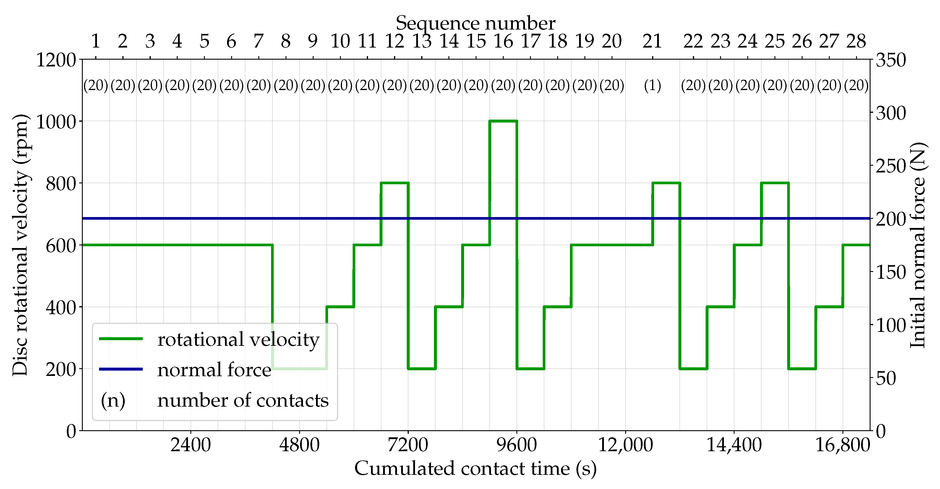
The experimental tests carried out are highly instrumented in order to characterize in details the emissions and the thermomechanical and vibratory response of the system. The noise emissions are recorded using a 50 kHz microphone located approximately 1 m away from the test bench.

Moreover, the near-surface temperature fields evolution is monitored using 16 thermocouples located within the pin. These thermocouples are located in depth near the surface, providing a detailed overview of the thermal phenomena occurring within the contact interface. Among the 16 thermocouples near the pin surface, 12 are located 2 mm beneath the surface, the other four are deeper; thus, only those 12 are considered for the investigation related in this paper. The layout of the thermocouples in the pin is illustrated in Figure 2c. The sampling frequency is 90 Hz.

In addition, the mechanical loading is tracked using three eddy-current sensors on the back of the pin, allowing for the measurement of the normal displacement and rotations of the pin. They are used in particular for the normal load enforcement, using the measured blade deflection and knowing its stiffness. The sensors have a sampling frequency of 50 kHz, allowing to capture the vibrational behavior of the system. The rotational velocity of the disc and the applied torque are measured as well. The instrumentation is illustrated in Figure 2a.

Finally, a discrete monitoring of the pin surface is carried out. After each test sequence, the system is left at rest to allow it to cool down completely. Then, a profilometry is performed using a focus-variation-based device (PortableRL, Alicona). The obtained surface profiles are processed in order to extract the macroscopic profile shape. This shape is obtained by fitting a degree-three polynomial over a centered 17 mm × 17 mm frame from the 20 mm × 20 mm surface. When removing this macroscopic shape, the remainder of the surface profile is referred to as the roughness profile. In addition to the surface profiles, optical images of the surface are made at the same time, providing a means of observation of the surface composition.

These measurements are completed by Scanning Electron Microscope (SEM) observations of the pin surface at the end of the test campaign.

2.4. Test Campaign

For the most part, the conducted tests consist of repeated short friction tests at a fixed disc rotational velocity. For each short friction test, the contact is maintained for 30 s, followed by a 10 s pause before the next contact. The initial normal load of each test is prescribed by adjusting the displacement of the blade extremities, then the normal displacement is maintained at its initial value throughout the test, allowing the normal force to vary slightly, mainly due to thermal expansion or wear. A sequence of 20 friction tests is performed under identical conditions (same rotational velocity and normal force), then the system is allowed to cool down completely. Thereafter, another test sequence is performed with a different rotational velocity. The process is depicted in Figure 3. The sequence 21 makes an exception: this specific sequence consists of a single contact maintained for 1200 s, able to reach high temperatures never seen before. During this individual contact, the disc rotational velocity is varied: it was fixed at 600 rpm for the first part of the contact, then shifted to 800 rpm for the second part of the contact. Overall, the test campaign consists of 28 sequences, of which 27 are composed of 20 short friction tests and one consists of a long-lasting contact.

The test conditions applied for each sequence are shown in Figure 3. Throughout the campaign, the initial normal load is $F_n=200$ N and the disc rotational velocity is varied between $\omega =200$ and $\omega =1000$ rotations per minute (rpm). The first seven sequences correspond to the running-in of the contact. Then, the successive sequences consist of low-velocity sequences followed by sequences of progressively higher rotational velocity. This way, the system undergoes increasingly higher loading levels. This pattern, with a progressive increase in the rotational velocity, is repeated several times.

The experimental tests conducted in this study are not strictly speaking braking tests, as the rotational velocity is maintained at a constant. However, the use of a pin-on-disc system that includes an actual brake disc and a pin machined from a commercial brake pad helps replicate the dynamical and tribological phenomena encountered in braking applications.

3. Global Results Analysis

The objective in this section is to provide a broad overview of the test results and to present a very global analysis of squeal events. The possible correlations between squeal occurrences and different global parameters (loading, coefficient of friction, temperature level) are also investigated. More detailed analyses of the results are conducted in Section 4.

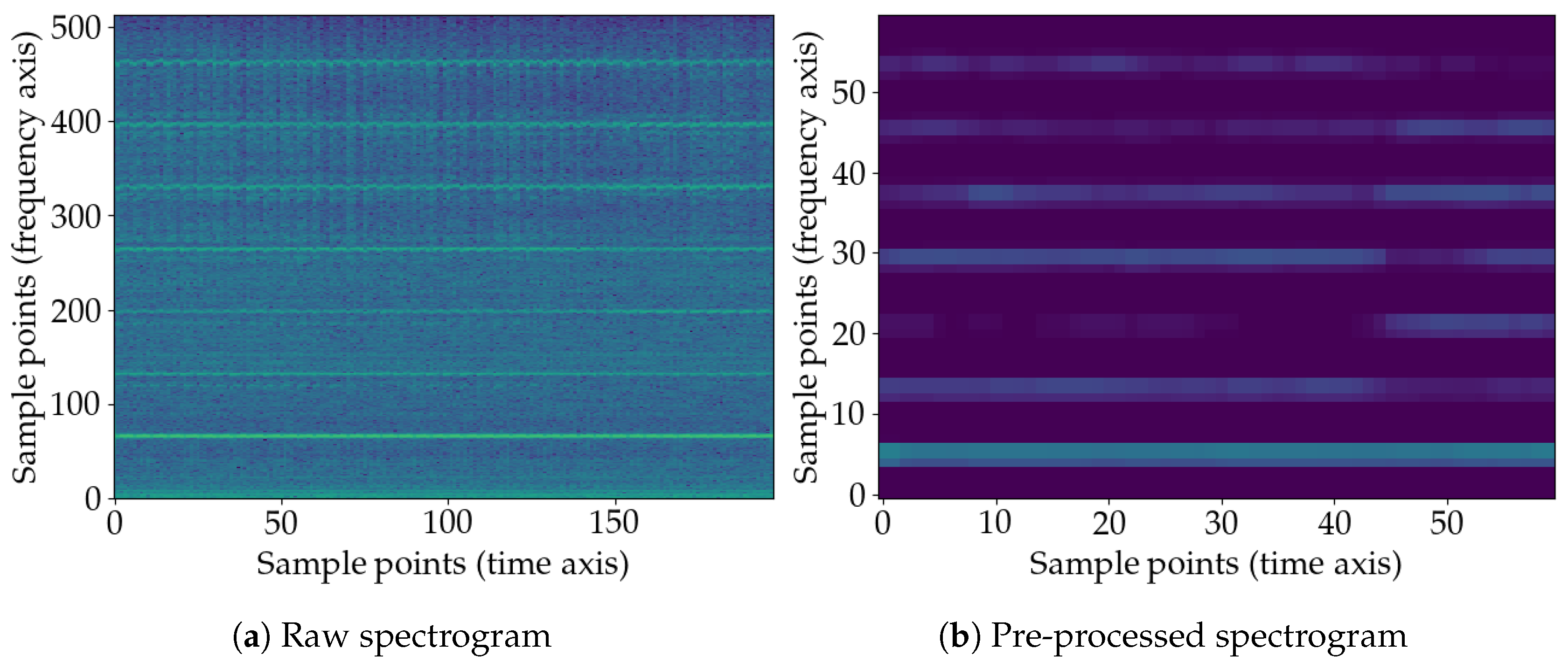
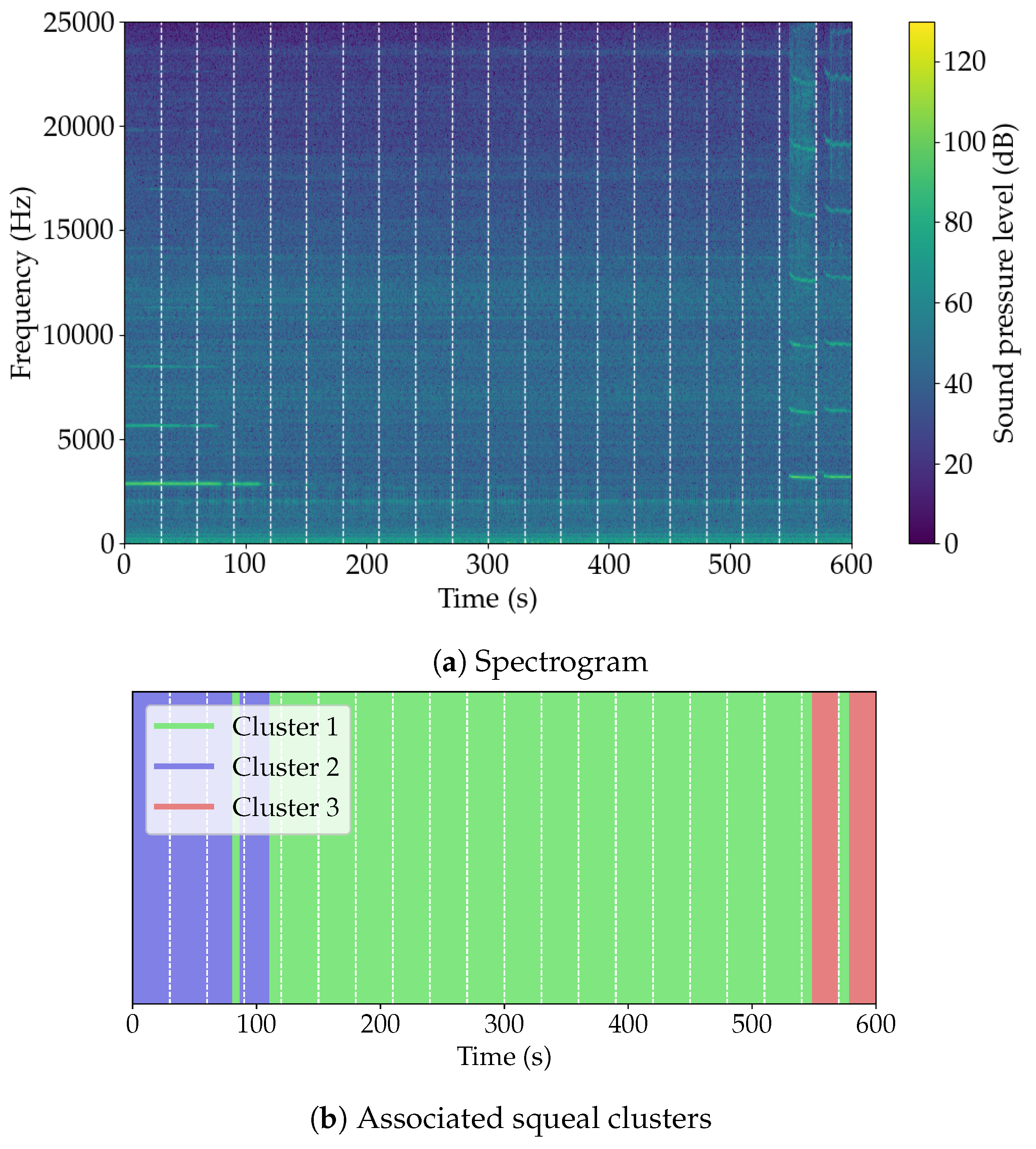
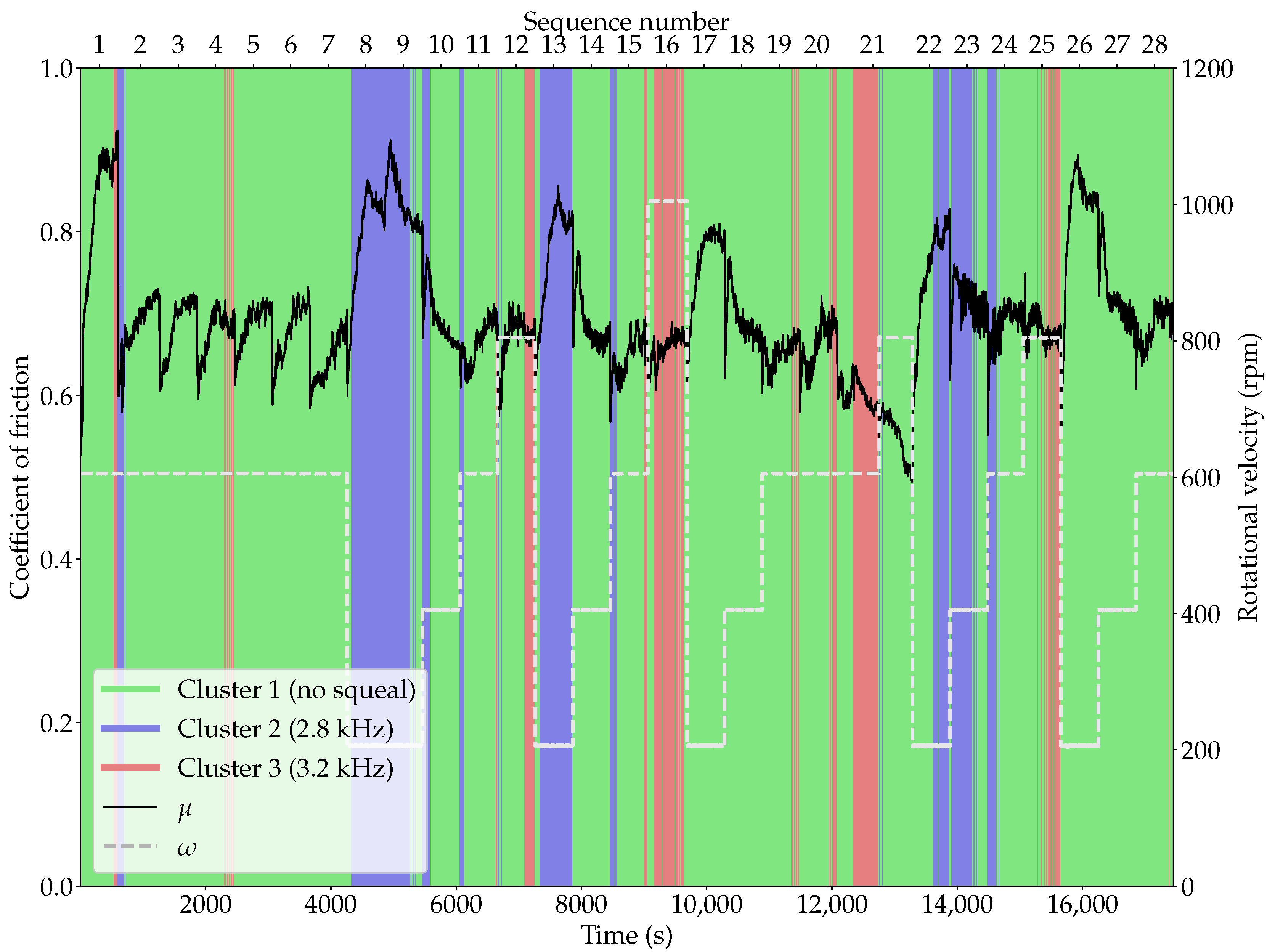
3.1. Analysis of Squeal Events

In order to characterize the squeal episodes occurring during the test campaign, the sound recordings are analyzed. For that, a short-time Fourier transform is used on the recorded sound time series to obtain sound spectrograms. The short-time Fourier transform is applied using a moving window with a Hann smoothing containing 1024 sampling points—corresponding to a 0.02 s window. This leads to the spectrogram representation showing the time and frequency evolution of the sound pressure level, in dB. The frequency content spans a range from 1 kHz to 25 kHz, the lower frequencies corresponding to the test bench noise being removed. An example of the sound pressure recorded by the microphone and the corresponding spectrogram is given in Figure 4.

This representation allows for clearly identifying two distinct squeal modes occurring during the campaign: the first one has a fundamental frequency around 2.8 kHz with few visible harmonics, the other has a fundamental frequency around 3.2 kHz with much more harmonics. A classification of the different squeal behaviors is then performed. Each friction test is decomposed into short time intervals of approximately 3 to 4 s, and each short time interval is assigned to a squeal class. The squeal classes aim at grouping together time intervals showing a similar squeal behavior.

The classification is carried out through a clustering technique using a k-means algorithm [28]. This unsupervised method aims at partitioning a set of data points, represented as vectors, into a given number k of subsets. The partition seeks to minimize the distance between the data points and the centroid of the cluster they belong to.

As the k-means algorithm relies on the $L^2$ norm to evaluate the proximity between two data points, a pre-processing of the spectrograms is required. Indeed, a point-by-point comparison of two spectrograms gives little to no information about the actual similarity of the squeal behaviors: such a comparison would label two similar spectrograms with only a slight difference in squealing frequency as completely different. As a consequence, the spectrogram’s pre-processing step is performed in order to correct this. First, a sound pressure level threshold is applied: every value below 70 dB is set to 0. Then, a Gaussian filter with a kernel size of $11\times 11$ is used. Finally, a max-pooling downsampling yields a coarser spectrogram with a final size of $60\times 60$, such that the k-means algorithm searches for clusters in a 3600-dimensional space (Figure 5). This way, the point-by-point comparison performed by the k-means algorithm would detect a close similarity between data with a reasonably close squealing frequency.

This squeal clustering process based on spectrograms is performed over the test campaign. As a rapid observation of the spectrograms throughout the campaign allows to identify three different squeal behaviors (absence of squeal, squeal at a $2.8$ kHz frequency and squeal at a $3.2$ kHz frequency), the k-means algorithm is used with $k=3$ clusters.

This results in a first cluster containing 4344 time intervals (74.7% of the 5818 data points) and representing the squeal-free situation (cluster 1), a second cluster with 922 time intervals (15.8%) corresponding to a $2.8$ kHz squeal (cluster 2), and a third cluster with 552 time intervals (9.49%) with a $3.2$ kHz squeal (cluster 3). The results are summarized in

Table 1. Results of the squeal clustering.

Cluster	Number of Time Intervals	Corresponding Squeal Mode
Cluster 1	4344 (74.7%)	No squeal
Cluster 2	922 (15.8%)	2.8 kHz
Cluster 3	552 (9.49%)	3.2 kHz

, and Figure 6b illustrates the clustering results on test sequence 15 as an example.

The time evolution of squeal clusters over the whole campaign is represented in Figure 7 together with the evolution of the coefficient of friction (evaluated from the torque and the normal force measurements considering a friction radius of 100 mm) and in Figure 8 along with the evolution of the measured temperatures below the pin surface. The figures also show the disc rotational velocity. The temperature evolution distinctly shows the sequence division: during each braking sequence, the measured temperatures rise progressively from the room temperature to higher levels, then return to the room level before the next sequence starts. Within each sequence, temperatures increase during each 30 s friction test, then decrease slightly upon the 10 s rest between each friction test, with every sequence, except sequence 21, being composed of 20 friction tests. As expected, the highest temperature levels are reached at the end of the sequences with the highest rotational velocity and of sequence 21 consisting of a maintained contact.

3.2. Relation Between Squeal and Loading

From Figure 7 and Figure 8, it can be concluded that the occurrences of $2.8$ kHz and $3.2$ kHz squeal episodes show no clear and direct correlation with the loading severity. Although $2.8$ kHz (represented by cluster 2, in blue in the figures) and $3.2$ kHz (represented by cluster 3, in red in the figures) squeal seem to occur more frequently at, respectively, low and high velocities, the sole consideration of the operating conditions does not allow for determining whether squeal occurs and, if so, at which frequency. For instance, it can be noticed that for sequence 12 ($\omega =600$ rpm) and sequence 15 ($\omega =800$ rpm), all three situations are met: no squeal, squeal at $2.8$ kHz, and squeal at $3.2$ kHz.

3.3. Relation Between Squeal and Friction

Figure 7 shows that the coefficient of friction $\mu$, which is calculated based on the measurements of the normal force and of the engine torque, presents a different behavior depending on the rotational velocity. It is indeed higher when the rotational velocity is lower: $\mu$ varies between 0.6 and 0.9 for $\omega =200$ rpm, while it comprises between 0.6 and 0.7 for higher rotational velocities. However, no clear correlation with squeal can be observed: both $2.8$ kHz squeal and $3.2$ kHz squeal may be found in a large range of coefficient of friction values over the campaign. This can be seen from the histogram of the coefficient of friction value, showing the three different squeal clusters (Figure 9a).

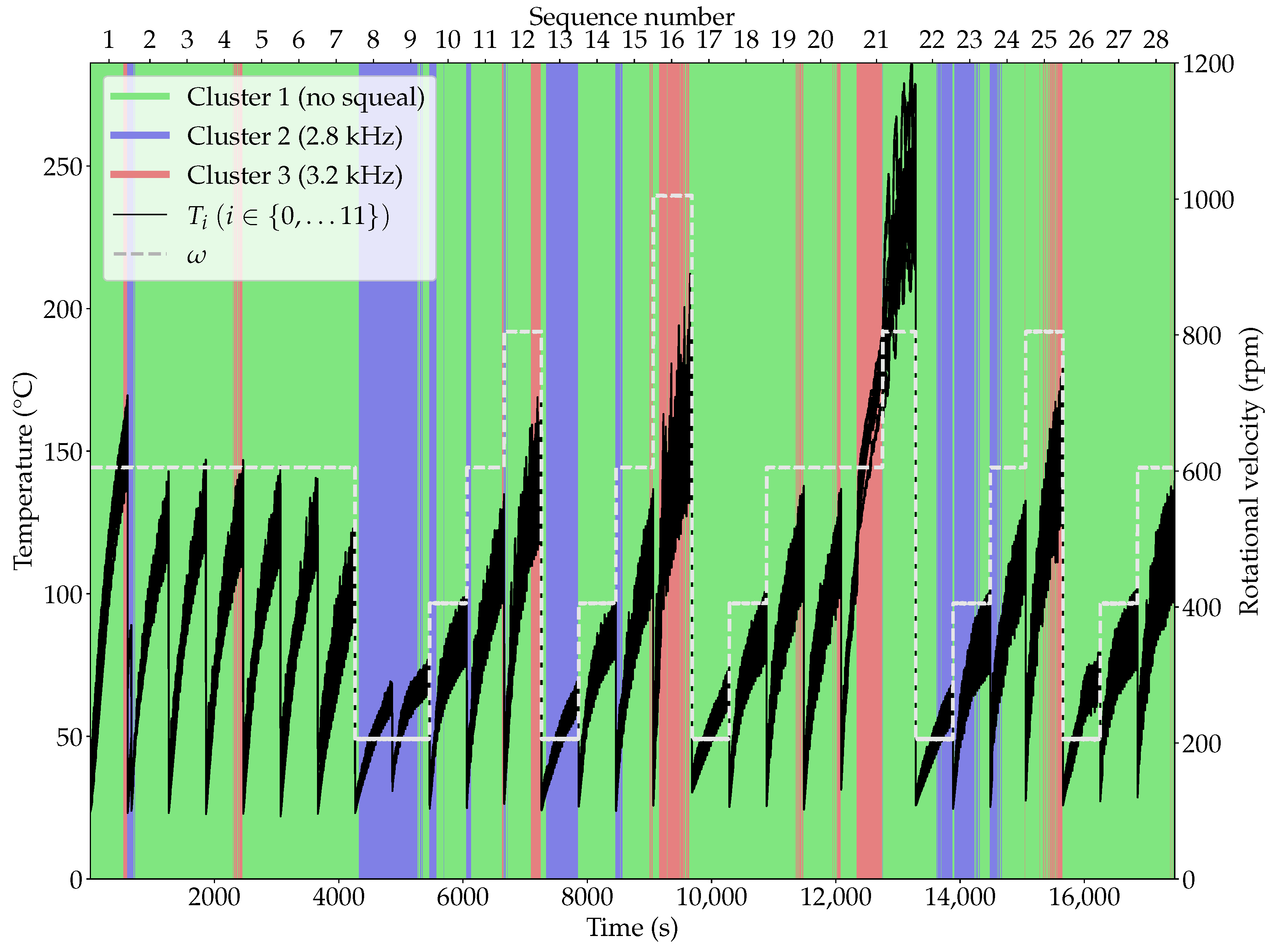
3.4. Relation Between Squeal and Temperature

In the temperature evolutions depicted in Figure 8, it is clear that the occurrences of $2.8$ kHz squeal (corresponding to cluster 2) and $3.2$ kHz squeal (corresponding to cluster 3) are closely related to the temperature level. The squeal mode with a $2.8$ kHz frequency is exclusively detected when the temperature level is low: that is, rather at the start of the test sequences and/or with a moderate rotational velocity; whereas the squeal mode with a $3.2$ kHz frequency occurs solely at high temperature levels (see, for example, sequences 12, 16, and 25). This first observation on the relation between the occurrence and nature of squeal and the level of temperature is consistent with the results obtained by [27]. A difference may however be observed in Figure 8 between the low-temperature $2.8$ kHz and the high-temperature $3.2$ kHz squeal: while $3.2$ kHz squeal seems to always appear as a certain temperature level is reached, $2.8$ kHz squeal seems more unpredictable. As an example, it can be observed that no squeal occurs during the low-temperature sequences 17 and 26, whereas $2.8$ kHz squeal occurs during sequences 13 and 22. This suggests that the squeal response is also subjected to a dependency on the history of the system loading, especially at low temperatures.

Figure 9b shows the histograms of the mean measured temperature for the data in each of the three clusters. While cluster 1, corresponding to the absence of squeal, spans the whole range of temperatures, it can clearly be seen that cluster 2 occurs only for low temperatures unlike cluster 3 that occurs only at high temperatures. The two clusters are fully disjoint in terms of temperature level. As a conclusion, the mean temperature level is indeed, in the present case, a sufficient parameter to discriminate between clusters 2 and 3. In this respect, it provides a first-order indicator of the squeal response of the system, which is consistent with the results obtained in [27]. However, it does not enable a complete determination of the squeal response, as the squeal-free situation may be found for all temperatures. This is particularly true for the lowest temperature levels: at low temperature, the squeal-free situation is at least as frequent as $2.8$ kHz squeal, while oppositely, the occurrence of $3.2$ kHz squeal is much more likely beyond a certain temperature. The few data over 200 °C which have no squeal (Figure 9b) make an exception, but are related to very specific test conditions: they correspond to the end of sequence 21 with a maintained contact and occurred right after the rotational velocity had been increased (see Figure 8). This rotational velocity change resulted in a rapid vanishing of squeal.

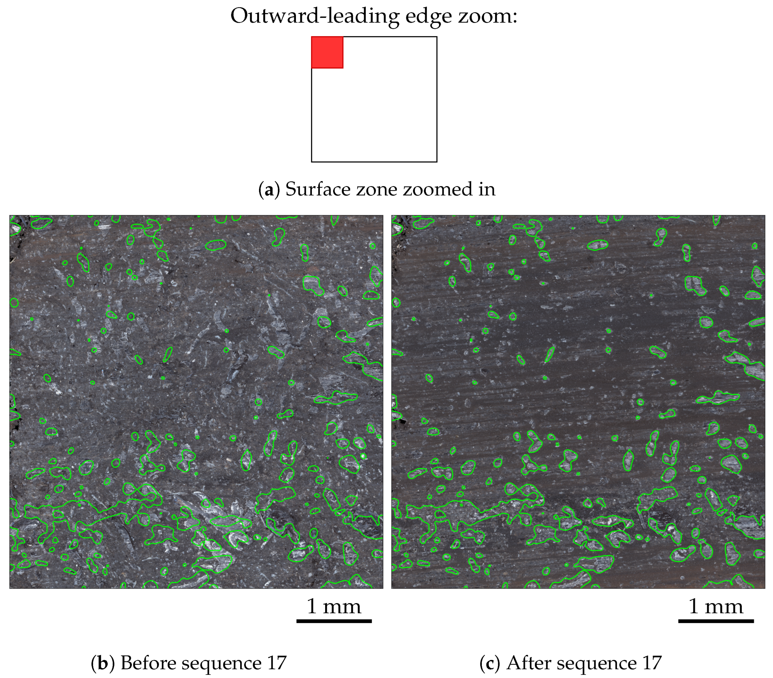
3.5. Surface Evolution

The observation of the pin surface between each test sequence shows that sequences with a high velocity produce very different surfaces from sequences with a low velocity. As an illustration, the evolution of the pin surface observed through optical images, and the evolution of the surface profile shape, is shown in Figure 10 over sequences 16 and 17. The surface profile shape is obtained as a degree-three polynomial over a 17 mm × 17 mm centered frame. The edges are not taken into account to suppress side effects in the polynomial fitting process which do not significantly affect the macroscopic shape. The surface edges are however accounted for in the squeal event analyses conducted in the next section. This example shows a typical transition from a high-velocity sequence to a low-velocity sequence, which is repeated several times throughout the campaign: sequence 16, with a high disc rotational velocity ($\omega =1000$ rpm) is followed by sequence 17 with a low rotational velocity ($\omega =200$ rpm).

The observation of the optical images shows that both high- and low-velocity sequences noticeably affect the surface. At the end of sequence 16, the steel fibers are very visible and very little powder is present on the surface. On the opposite, the comparison between the end and the start of sequence 17 shows that the low-velocity sequence has led to a large amount of powdery material on the surface, which is visible as the darker homogeneous areas, mostly in the center of the pin surface. The observation of the surface shape, which is obtained through a degree-three polynomial fit, is also very insightful. First, it can be noticed that the surface has a hollow shape: the center of the surface is deeper than the edges. This global shape, measured when the pin has cooled down, does not change with the sequence. However, its magnitude changes significantly: high-velocity sequence 16 produces a much more hollow surface than initially. Oppositely, low-velocity sequence 17 has flattened the surface: the shape magnitude is much lower after than before the sequence. The overall surface shape has however not changed: the surface still presents a hollow shape, but its magnitude is lower.

The fact that high-temperature sequences produce very hollow surfaces on the pin may be understood based on thermomechanical considerations. The local temperature elevations measured on the thermocouples in the pin are represented for different instants of sequence 16 in Figure 11. It shows that the temperature elevation is very localized in the center of the pin surface, suggesting a very localized contact. It can therefore be assumed that due to the high rotational velocity and the high temperature levels, the pin is thermally deformed, producing significant wear in the center of the surface where the contact is localized. This process is schematically depicted in Figure 12: the initial surface is hollow, but due to the severe temperature increase, the contact readily occurs mostly in the center of the pin surface, producing an even more hollow surface shape when the pin has cooled down due to wear.

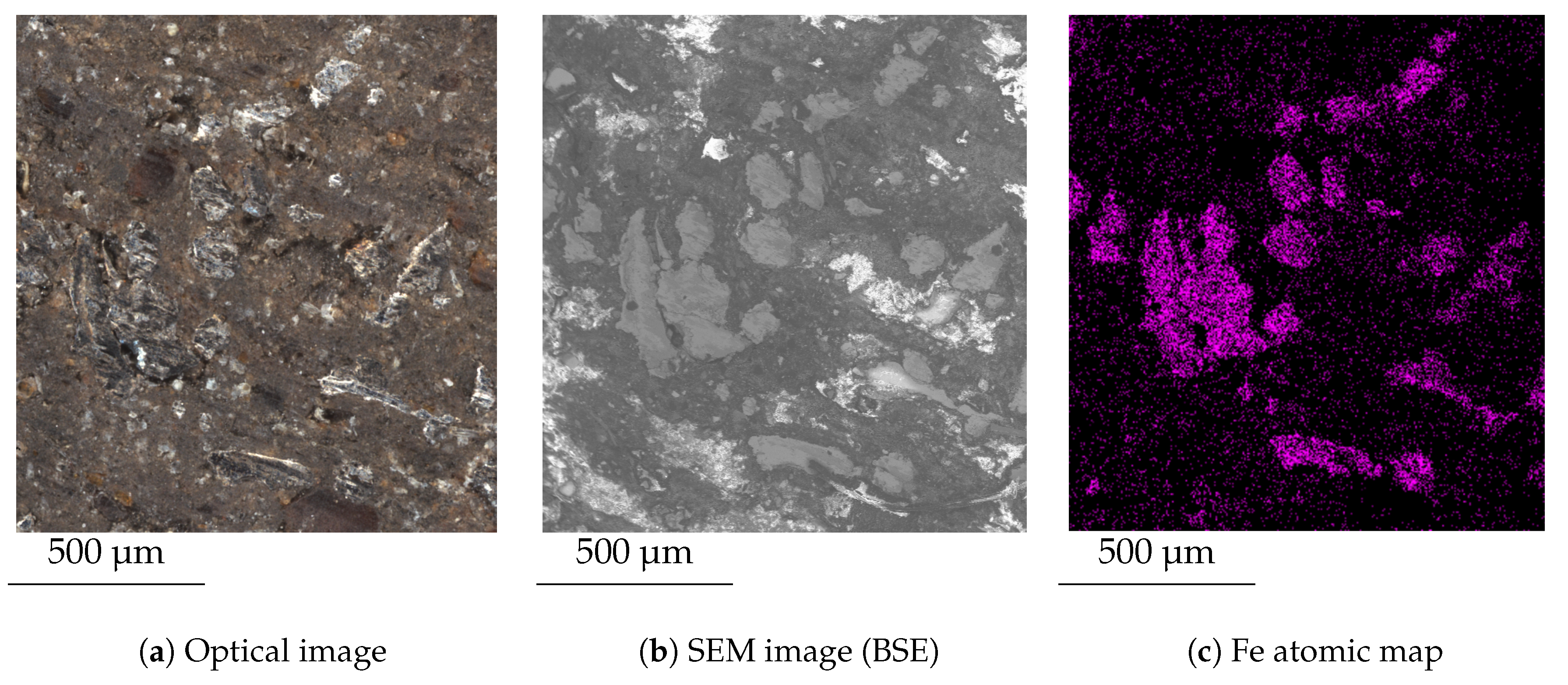
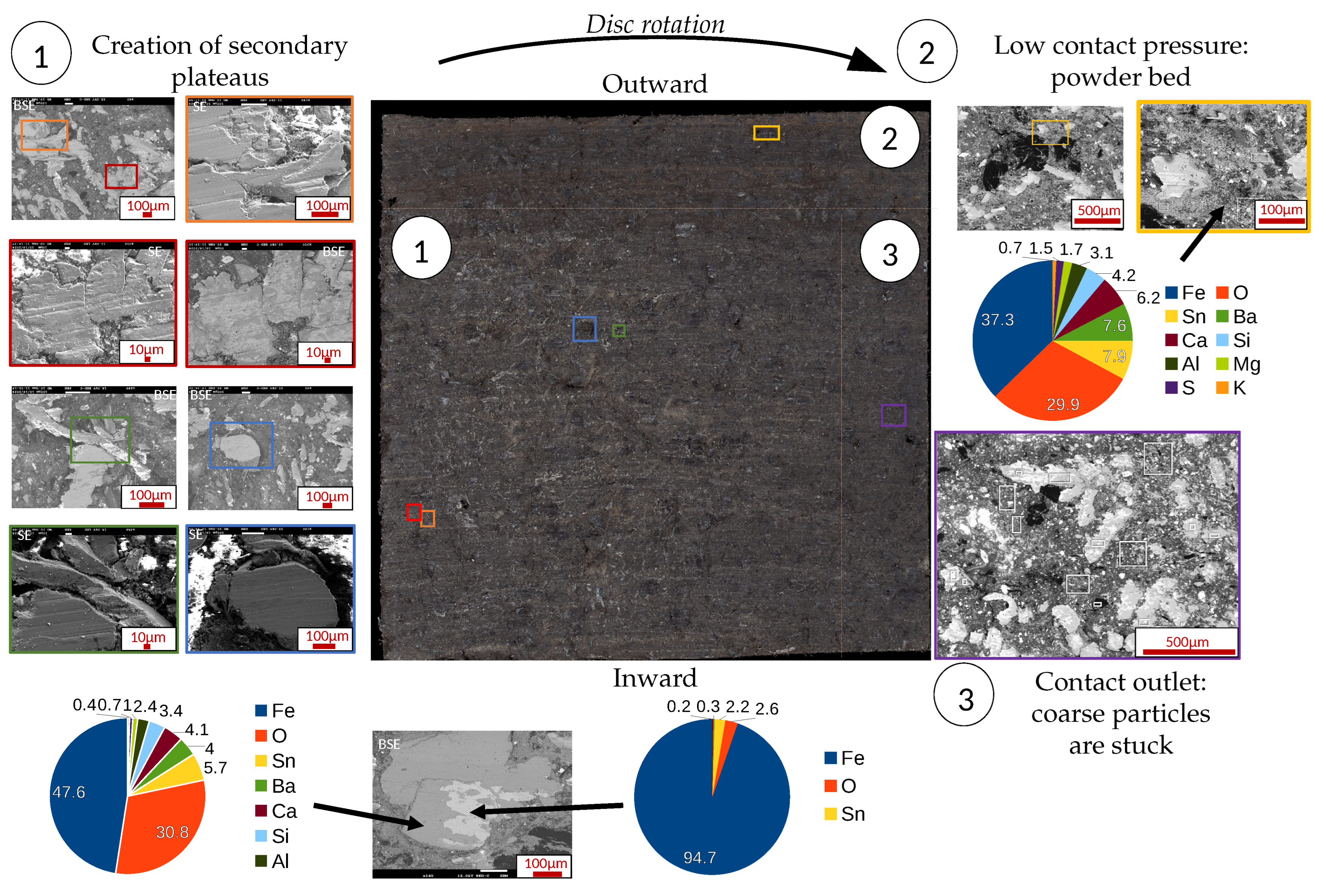
3.6. Postmortem Surface Analysis

SEM analysis of the pin surface is conducted at the end of the test campaign. The objective is to try to identify indicators of the tribological contact conditions. The aim of the SEM analysis is to help interpret the observations made on optical images of the surface taken throughout the campaign. The SEM observations are summarized in Figure 13. This analysis was carried out just after a test with a maintained contact, during which high temperature levels were reached. On this surface, three different zones are identified.

The first zone covers most of the surface and shows secondary load-bearing plateaus located on the steel fibers or nearby them. Chemical composition analyses allow for distinguishing uncovered steel fibers, which are mostly made of iron and visible in lighter gray on backscattered electron (BSE) images, from the secondary plateaus in darker gray on BSE images, made of oxidized iron and additional elements. The chemical composition of secondary plateaus is similar to the composition of loose third body particles, indicating that these plateaus are formed from compacted third body particles, coming either from the pin or from the disc. Secondary electron (SE) images allow for seeing the surface topography more clearly and show sliding tracks on the secondary plateaus. These observations led to the conclusion that this wide first zone was the location of high contact pressures, and that on a microscopic scale, the contact is localized on the steel fibers.

A second zone, located outward, is identified in which the surface is covered with a powdery material bed. In this zone, the contact pressure was lower, and third body particles had not been compacted. No load-bearing plateaus were found in this area.

The third zone is located at the rear, where coarser particles are found. These particles were stuck within the contact and were not able to be ejected due to their sizes.

The observations made based on the SEM analysis mainly allowed for concluding that on a microscopic scale, the contact occurs on the steel fibers. This observation is used in the following when analyzing the optical images of the pin surface between each sequence.

4. Focus on Squeal at Low Temperature

From the global analysis of the results, it appears that the conditions of occurrence of $2.8$ kHz squeal require further investigation in order to be elucidated, in comparison with $3.2$ kHz which always occurs as a certain temperature level is reached. Consequently, in the remainder of the paper, the focus is set on the low-temperature $2.8$ kHz squeal. The investigation on the conditions of its occurrence is based on several sequences at low rotational velocities, namely sequences 13, 17, 22, and 26. All these sequences, albeit with the same loading level and disc rotational velocity, show a very different squeal response: while $2.8$ kHz squeal occurs during sequences 13 and 22, this is not the case for sequences 17 and 26.

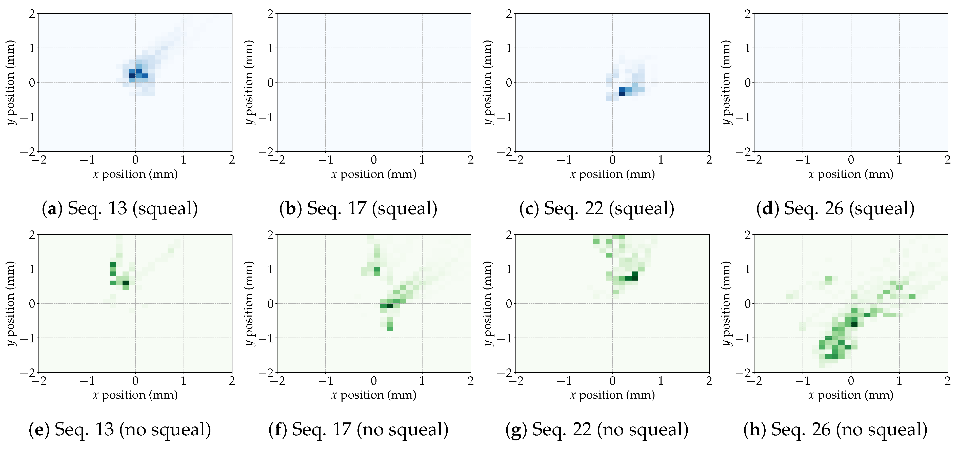
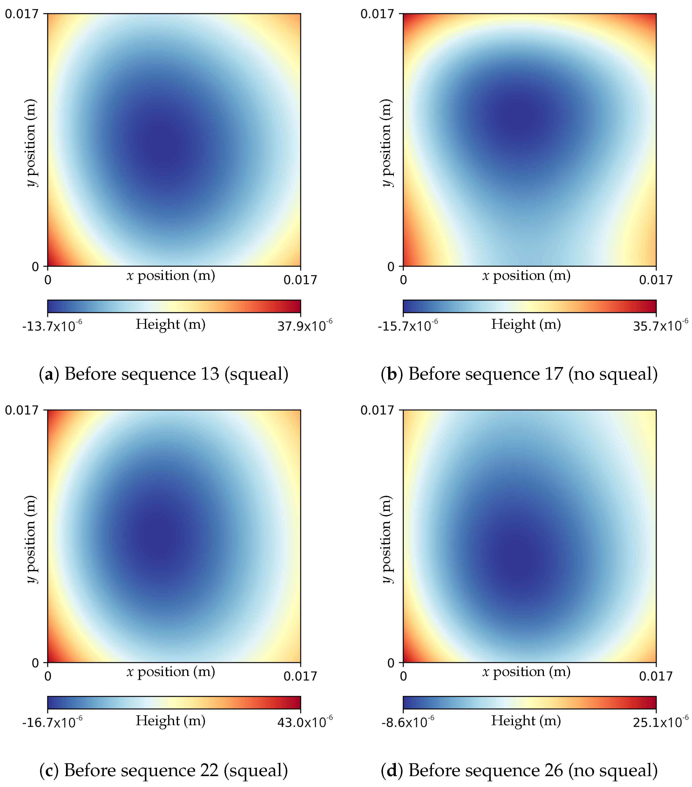
4.1. Detailed Surface Analysis

As a first step, a more detailed comparison of the pin surfaces before and after the low-velocity sequences is conducted. For instance, this comparison is presented for sequence 17, but similar conclusions are drawn for the other low-velocity sequences investigated. The optical images and profile shapes of the pin surface are shown in Figure 10 for the start and end of sequence 17.

A zoom in on the center of the surface is shown in Figure 14. It can be observed that this area is different after the sequence from before the sequence: it is covered with large, darker and more homogeneous zones, which are identified as powder beds. However, the steel fibers, located by the small lighter shapes, display a very similar layout. In order to visualize it, a detection of the fibers boundaries is performed on the surface image at the end of the sequence, and the obtained contours are reported on the initial surface image (green contours in the figure). It can be seen that the steel fibers have not been altered over the sequence in this central surface zone: all the steel fibers detected on the surface image after the sequence were already present before the sequence. On the opposite, some initially visible fibers are not retrieved at the end. They are likely covered by the large powder beds. As it is known from the SEM analysis (Section 3.6) that the contact is mainly established on the steel fibers on a microscopic scale, it can be inferred that over this test sequence, the contact has locally barely occurred in the center of the surface as the fibers seem intact.

Conversely, the observation of the external zones of the surface shows a much greater alteration of the steel fibers. For instance, Figure 15 shows a zoom in on a surface corner, located near the outward and leading edges. This time, the steel fibers detected at the end cannot be found on the initial surface and, conversely, the fibers that were initially present on the surface cannot for the most part be retrieved at the end of the sequence. A similar observation is made on all corners of the surface. This suggests that over this sequence, the sides and corners of the surface have carried contact load, contrarily to the center of the surface.

As it was observed in Section 3.5 on the pin surface profile shape evolution, the resulting surface after sequence 17 is much flatter than before the sequence, where the surface is very hollow due to the preceding severe loading. The fact that the center of the surface is covered with powdery material at the end of the sequence can partly explain why the surface at the end is flatter than before, in addition to wear on the edges and corners of the surface.

The surface observation presented here for sequence 17 was also conducted for the low-velocity sequences 13, 22, and 26, which showed very similar features: the central part of the surface contains a significant amount of third body particles, and shows no trace of contact localization; the steel fibers seem almost intact. On the opposite, the external parts show an alteration of the steel fibers over the sequence, indicating zones over which contact was established. This is consistent with the surface shapes, which are initially very hollow before these sequences, leading to a localized contact on the edges and corners. After the sequences, the surface shape is much flatter, which is likely the result of wear on the edges combined with the accumulation of trapped third body particles in the center of the surface. These observations are common for all low-velocity sequences and do not allow for differentiating sequences during which squeal occurred from sequences during which it did not.

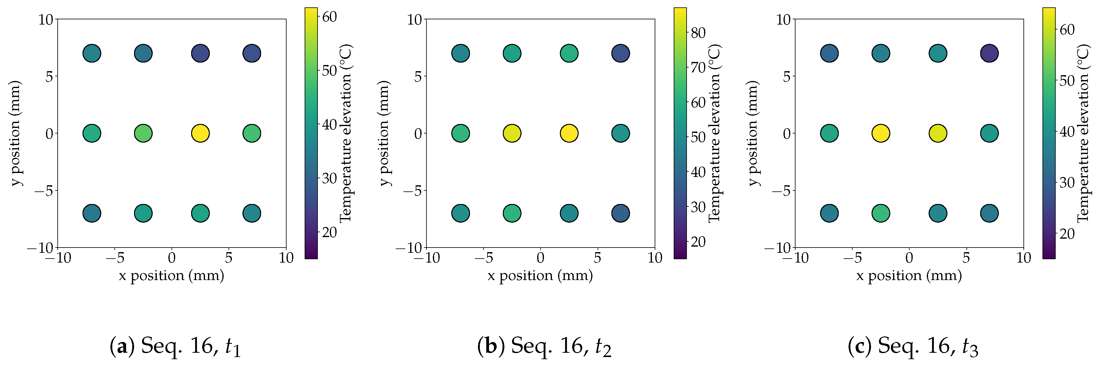
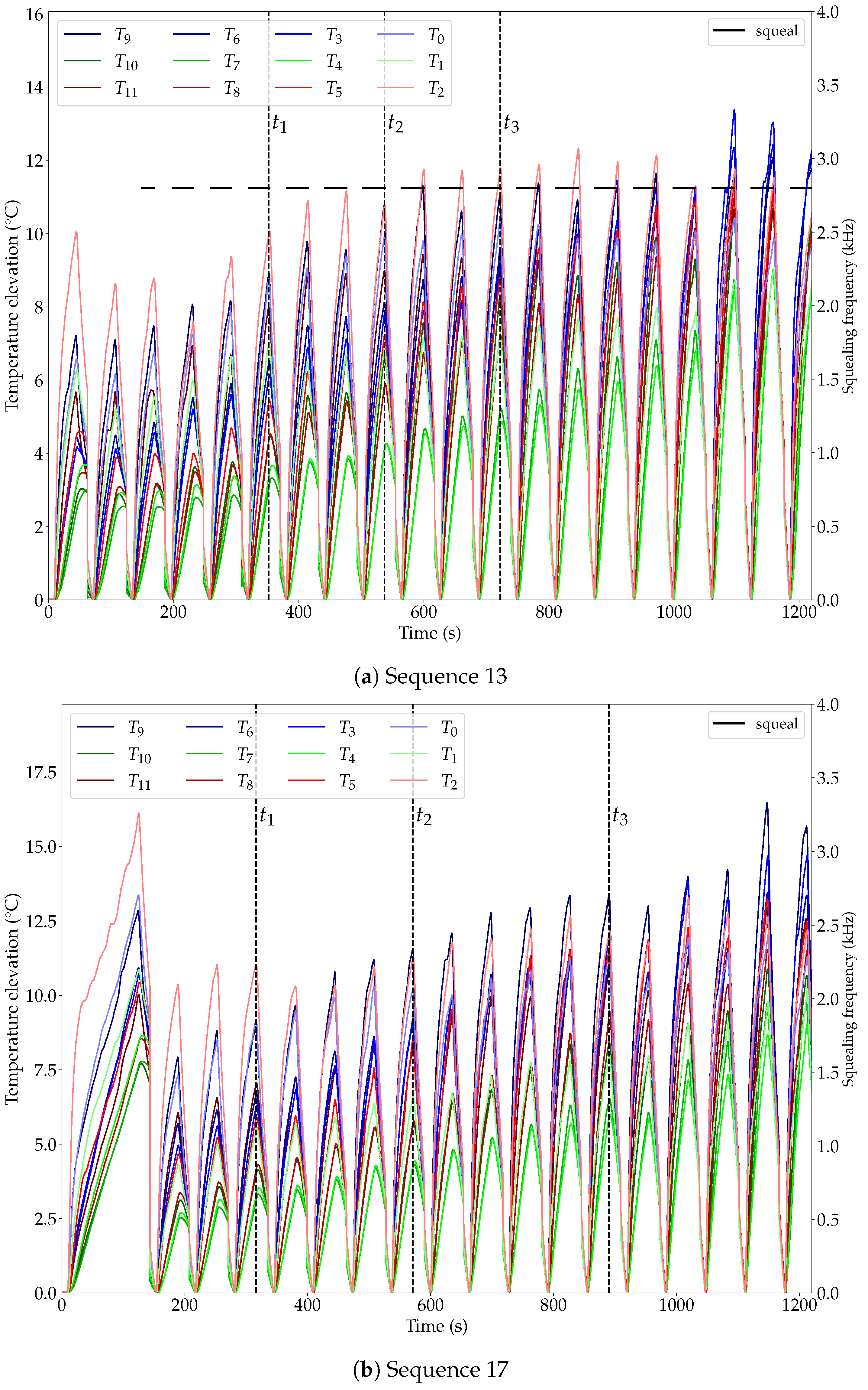
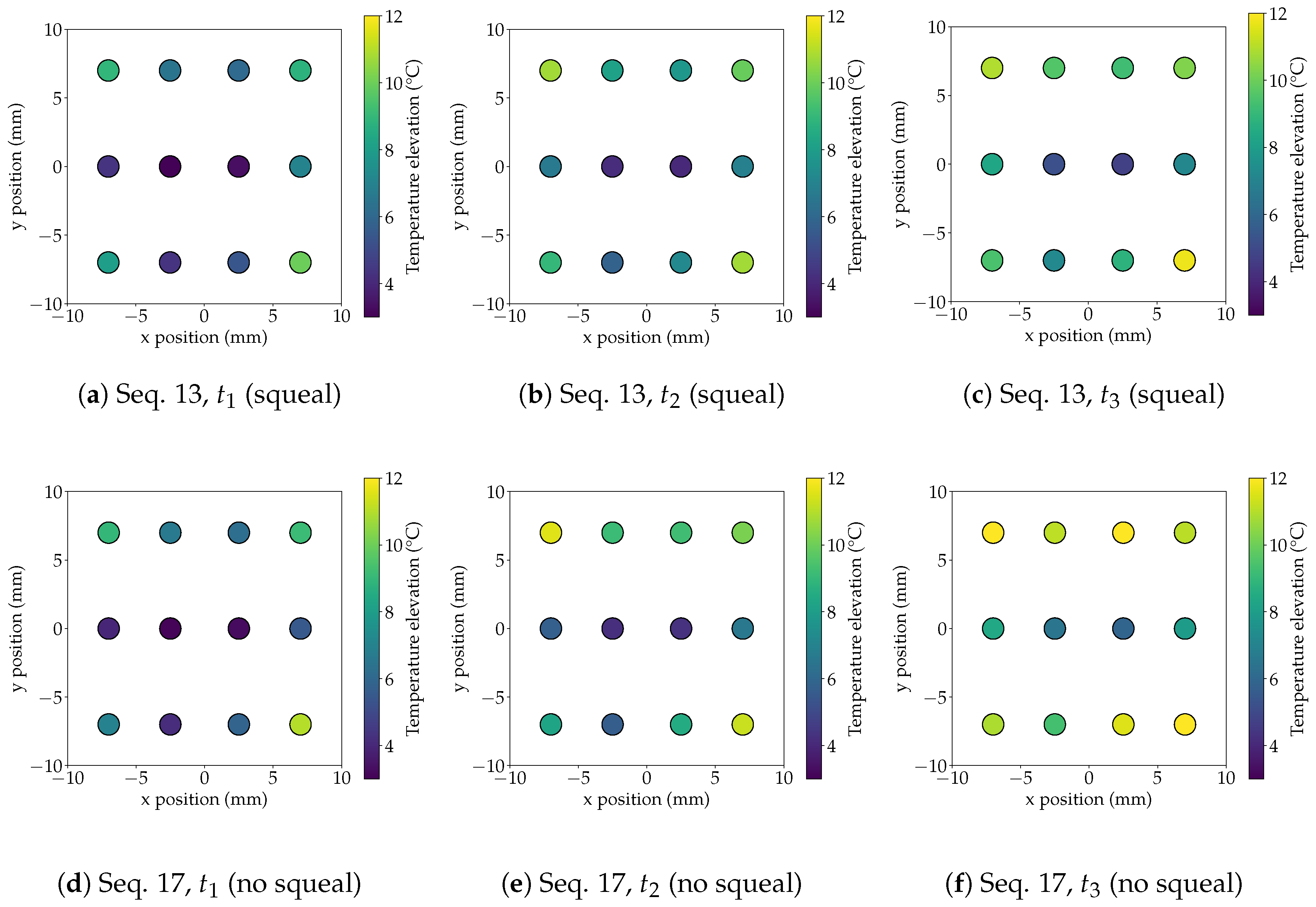
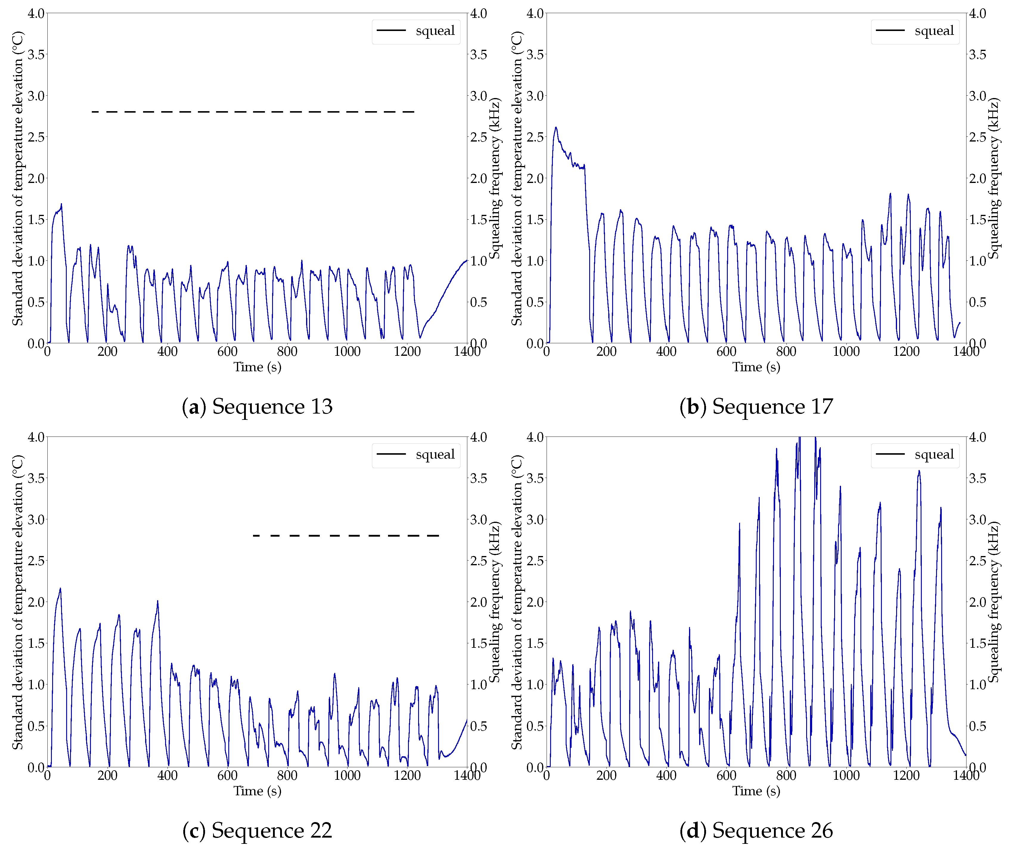
4.2. Evolution of Local Temperature Elevation

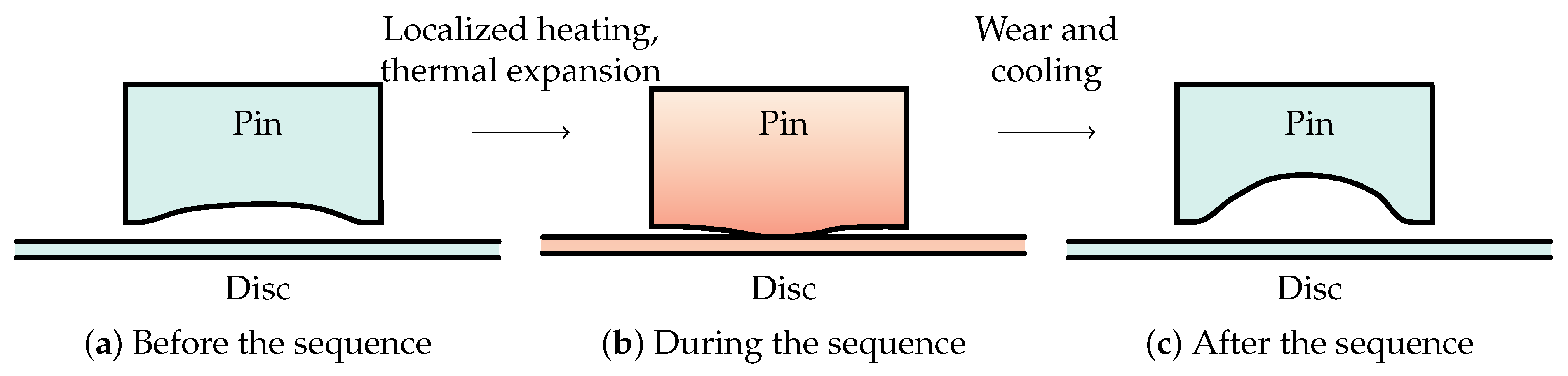
In order to support the analysis based on the surface observation, a detailed study of the temperature evolution in the pin is performed. Using the 12 thermocouples located 2 mm beneath the surface allows for obtaining a detailed mapping of the local distribution of temperature evolution, which gives information about the surface localization of energy dissipation.

In order to study the distribution of temperature increase during each contact, we consider the local temperature elevation $\Delta T_i$ over 30 s friction tests, for each thermocouple $i\in \{0,\dots ,11\}$:

$$\Delta T_i\left(t\right)=T_i\left(t\right)-T_{i,0}\mathrm{for}i\in \{0,\dots ,11\}$$

(1)

where $T_{i,0}$ is the temperature measured by the ith thermocouple at the start of the current contact. The temperature elevation is used as an indicator instead of the temperature level, as it allows for better capturing where the contact is mostly localized during each single friction test. This indicator starts from zero at the beginning of each friction test, then increases progressively during the contact and is set to zero again at the start of the next contact.

The evolution of local temperature elevations is depicted in Figure 16 for low-velocity sequences 13 (during which squeal occurs, as represented in the figure) and 17 (during which no squeal occurs). It can be seen that the highest temperature elevations are mostly localized on the thermocouples located near the four edges (thermocouples 0, 2, 9, and 11). As discussed in the previous section, the initial surface profile for these sequences is always very hollow: the center of the surface is much deeper than the edges (see Figure 10 and Figure 12). This explains why these sequences have a contact which is initially localized on the corners. On the opposite, the temperature elevation measured near the surface center (thermocouples 4 and 7) is significantly lower. This confirms the conclusions drawn from the surface analysis: during these low-velocity sequences, no contact is established in the center of the surface. This localization on the surface corners of temperature increase holds for the whole duration of the sequence. This can suggest that the loading is not severe enough to generate sufficient wear and thermal expansion for the contact to change its localization. In addition, it can also be seen in Figure 16 that the temperature elevation during each 30 s contact progressively increases from the start of the sequence to the end.

This corner contact localization can also be visualized on temperature elevation maps shown at snapshots $t_1$, $t_2$, and $t_3$ as defined in Figure 16 and shown in Figure 17. This representation makes clearly visible the high temperature increase on the edges, which contrasts with the surface center where the temperature elevation is very limited. In this figure, while the corner localization can be observed for both sequences 13 and 17, it appears that the distribution of temperature elevation over the four corners seems to be more balanced for sequence 13 (during which squeal occurs) than for sequence 17 (during which no squeal occurs).

This difference in the distribution of temperature elevation over the four corners between situations with squeal and the situations without squeal is repeated for all low-velocity sequences. In order to illustrate this, the center of gravity of temperature elevation over the four corners is considered as an indicator of the balance of temperature elevation. The x and y coordinates of this center of gravity are calculated as follows:

$$\begin{array}{cc}\hfill \overline{x_{\Delta T}}& ={\displaystyle \frac{x_0\Delta T_0+x_2\Delta T_2+x_9\Delta T_9+x_{11}\Delta T_{11}}{\Delta T_0+\Delta T_2+\Delta T_9+\Delta T_{11}}}\hfill \end{array}$$

(2)

$$\begin{array}{cc}\hfill \overline{y_{\Delta T}}& ={\displaystyle \frac{y_0\Delta T_0+y_2\Delta T_2+y_9\Delta T_9+y_{11}\Delta T_{11}}{\Delta T_0+\Delta T_2+\Delta T_9+\Delta T_{11}}}\hfill \end{array}$$

(3)

with the thermocouples on the four corners numbered 0, 2, 9, and 11. This way, values of $\overline{x_{\Delta T}}$ and $\overline{y_{\Delta T}}$ close to zero indicate that the contact is well balanced over the four corners, while higher values indicate an imbalance. This indicator is represented for different low-velocity sequences in Figure 18, which represents two-dimensional histograms (heatmaps) of $\overline{x_{\Delta T}}$ and $\overline{y_{\Delta T}}$. They are built by considering one point every 0.5 s. For sequences 13 and 22, the center of gravity values is gathered around zero when squeal occurs, indicating that the four corner thermocouples measure a very close temperature elevation value. Oppositely, for all the sequences, the histogram is more spread in both x and y directions when squeal does not occur. This indicates that the temperature elevation measured by the four corner thermocouples are quite different: a higher x value refers to a contact localization closer to the trailing edge, while a higher y value refers to a contact localization closer to the outward edge. This observation confirms that when $2.8$ kHz squeal occurs, the temperature elevation is always evenly balanced over the four corners, which is not the case in the absence of squeal.

Another illustration of this is provided by the evolution of the standard deviation of the temperature elevation, depicted in Figure 19. The standard deviation is calculated from the temperature elevation values measured on the four corner thermocouples. The times at which squeal occurs are represented as well. It can be observed that squeal occurs only when the standard deviation of the temperature elevation does not exceed 1 °C. Conversely, when standard deviation values are greater, squeal never occurs. This representation allows for seeing the time evolution: for sequence 22, squeal does not occur at the start when the temperature elevation is not well balanced over the corners. Then, from the middle of the sequence, the standard deviation decreases meaning that the four temperature elevation values are close, and squeal appears. This confirms that $2.8$ kHz squeal is correlated with a rather uniformly distributed temperature elevation over the pin surface corners.

This difference in the balance of contact localization over the corners is likely related to different surface shapes. Figure 20 shows the initial surface profile shapes before sequences 13, 17, 22, and 26, approximated as degree-three polynomials. For sequences 13 and 22, during which squeal occurs, it can be seen that the profile has a very regular and symmetric shape: it is deeper in the center and more elevated towards the edges and corners with a similar progression in all directions. On the opposite, for sequence 17 and, to a lesser extent, sequence 26, during which squeal did not occur, the initial surface shape is not symmetric. Both show indeed an opening on one of the side edges: for sequence 17, the inward edge (bottom of the image) is much deeper than the rest, while the outward edge (top of the image) is deeper for sequence 26. This observation corroborates the differences highlighted on the temperature elevations between these four sequences: squeal occurs during sequences that have a more balanced temperature elevation over the corners, related to a more evenly distributed contact, which is consistent with more symmetric initial surface profiles.

4.3. Discussion

The combined analysis of temperature elevation distribution and the evolution of surface composition and shapes provides corroborating evidences suggesting that the contact conditions on a macroscopic scale drive the occurrences of squeal. The two squeal modes identified are found to occur under specific contact localizations, and regarding the low-temperature 2.8 kHz squeal, the evolution of the macroscopic load-bearing area is found to affect the squeal propensity. Based on these observations, it is possible to infer the influence of the loading level on the macroscopic contact conditions and squeal.

It is observed that $3.2$ kHz squeal always occurs when a certain temperature level is reached and is therefore easier to predict. This can be understood considering that thermal expansion and wear are prevalent features during tests at a severe loading and govern the evolution of the load-bearing area. Thus, the system evolution during the contact is likely to prevail over the initial conditions, which have a limited influence on the occurrences of squeal as they are rapidly erased by the contact evolution. On the opposite, it is observed that during low-velocity tests, the occurrence of 2.8 kHz squeal is more unpredictable: it may or may not occur during tests with the same loading. The analysis of this squeal mode shows that its occurrence is dependent on the initial conditions, especially regarding the macroscopic pin surface profile shape. This dependency can be interpreted by the fact that thermal expansion and wear arguably have a much lower or slower impact in this case. As a consequence, the contact localization is very stable: it holds on the edges and corners for almost the whole duration of a sequence, and the initial contact state has therefore a key role.

This is furthermore consistent with the fact that 2.8 kHz squeal can more briefly occur at the beginning of high-velocity sequences and then quickly cease (see, for instance, sequence 12 at $\omega =800$ rpm, or sequence 15 at $\omega =600$ rpm, Figure 8). The initial conditions before these sequences may favor the occurrence of $2.8$ kHz squeal, which is triggered at the start of the sequence but rapidly stops due to the severe loading, which quickly affects the contact conditions.

5. Conclusions

The pin-on-disc experimental tests conducted in this study enabled a precise investigation of the conditions of brake squeal occurrence. Two different squeal modes are observed during the tests: one at a $2.8$ kHz frequency and the other at a $3.2$ kHz frequency. The thermal measurements show that the mean temperature level in the vicinity of the pin surface provides a first-order indicator of the squeal mode: whereas $2.8$ kHz squeal is solely obtained for low temperatures, $3.2$ kHz squeal occurs exclusively at high temperatures. However, regarding the low-temperature $2.8$ kHz squeal, it appears that sequences showing a similar global temperature evolution could lead to different squeal responses.

An in-depth analysis of the evolution of macroscopic contact localization provides valuable insights into the contact conditions leading to the occurrence of $2.8$ kHz squeal. The combined analysis of surfaces and temperature evolutions allows for tracking the evolution of the macroscopic contact localization, which is shown to be closely related to squeal episodes. It appears that during the low-velocity sequences, the contact is very localized on the corners, due to the initially very hollow surface. As there is limited wear and thermal expansion during these low-velocity sequences, the contact holds on the corners for the whole duration of the sequences. As a result, the occurrences of $2.8$ kHz squeal are closely related to the initial macroscopic surface conditions. The analyses also allow to relate this initial surface conditions to the history of past loading: high-velocity sequences produce very hollow surfaces, while low-velocity sequences tend to flatten the surface. The evolution of the pin surface initial shape thus appears to depend on the thermomechanical and tribological processes that took place during the previous friction tests.

In order to understand in more detail the thermomechanical effects that govern the evolution of macroscopic load-bearing area, ongoing work is devoted to the development of numerical models accounting for thermal effects and wear. This will allow for studying the evolution of contact localization based on the loading history in greater detail.

References

1. Oesterle, W.; Doerfel, I.; Prietzel, C.; Rooch, H.; Cristol-Bulthe, A.L.; Degallaix, G.; Desplanques, Y. A comprehensive microscopic study of third body formation at the interface between a brake pad and brake disc during the final stage of a pin-on-disc test. Wear 2009, 267, 781–788. [Google Scholar] [CrossRef]
2. Candeo, S.; Leonardi, M.; Gialanella, S.; Straffelini, S. Influence of contact pressure and velocity on the brake behaviour and particulate matter emissions. Wear 2023, 514, 204579. [Google Scholar] [CrossRef]
3. Kinkaid, N.; O’Reilly, O.; Papadopoulos, P. Automotive disc brake squeal. J. Sound Vib. 2003, 267, 105–166. [Google Scholar] [CrossRef]
4. Akay, A. Acoustics of friction. J. Acoust. Soc. Am. 2002, 111, 1525–1548. [Google Scholar] [CrossRef]
5. Hoffmann, N.; Fischer, M.; Allgaier, R.; Gaul, L. A minimal model for studying properties of the mode-coupling type instability in friction induced oscillations. Mech. Res. Commun. 2002, 29, 197–205. [Google Scholar] [CrossRef]
6. Sinou, J.J.; Jezequel, L. Mode coupling instability in friction-induced vibrations and its dependency on system parameters including damping. Eur. J. Mech. A-Solids 2007, 26, 106–122. [Google Scholar] [CrossRef]
7. von Wagner, U.; Hochlenert, D.; Hagedorn, P. Minimal models for disk brake squeal. J. Sound Vib. 2007, 302, 527–539. [Google Scholar] [CrossRef]
8. Stender, M.; Tiedemann, M.; Spieler, D.; Schoepflin, D.; Hoffmann, N.; Oberst, S. Deep learning for brake squeal: Brake noise detection, characterization and prediction. Mech. Syst. Signal Process. 2021, 149, 107181. [Google Scholar] [CrossRef]
9. Eriksson, M.; Jacobson, S. Friction behaviour and squeal generation of disc brakes at low speeds. Proc. Inst. Mech. Eng. Part D-J. Automob. Eng. 2001, 215, 1245–1256. [Google Scholar] [CrossRef]
10. Sinou, J.J.; Lenoir, D.; Besset, S.; GilIot, F. Squeal analysis based on the laboratory experimental bench “Friction-Induced Vibration and noisE at Ecole Centrale de Lyon” (FIVE@ECL). Mech. Syst. Signal Process. 2019, 119, 561–588. [Google Scholar] [CrossRef]
11. Bergman, F.; Eriksson, M.; Jacobson, S. The effect of reduced contact area on the occurrence of disc brake squeals for an automotive brake pad. Proc. Inst. Mech. Eng. Part D-J. Automob. Eng. 2000, 214, 561–568. [Google Scholar] [CrossRef]
12. Chen, G.; Zhou, Z.; Kapsa, P.; Vincent, L. Effect of surface topography on formation of squeal under reciprocating sliding. Wear 2002, 253, 411–423. [Google Scholar]
13. Hetzler, H.; Willner, K. On the influence of contact tribology on brake squeal. Tribol. Int. 2012, 46, 237–246. [Google Scholar] [CrossRef]
14. Kennedy, F.E.; Ling, F.F. A Thermal, Thermoelastic, and Wear Simulation of a High-Energy Sliding Contact Problem. J. Lubr. Technol. 1974, 96, 497–505. [Google Scholar] [CrossRef]
15. Eriksson, M.; Bergman, F.; Jacobson, S. On the nature of tribological contact in automotive brakes. Wear 2002, 252, 26–36. [Google Scholar] [CrossRef]
16. Massi, F.; Berthier, Y.; Baillet, L. Contact surface topography and system dynamics of brake squeal. Wear 2008, 265, 1784–1792. [Google Scholar] [CrossRef]
17. Godet, M. The third-body approach: A mechanical view of wear. Wear 1984, 100, 437–452. [Google Scholar] [CrossRef]
18. Berthier, Y. Maurice Godet’s Third Body. In The Third Body Concept Interpretation of Tribological Phenomena; Dowson, D., Taylor, C.M., Childs, T.H.C., Dalmaz, G., Berthier, Y., Flamand, L., Georges, J.M., Lubrecht, A.A., Eds.; Tribology Series; Elsevier: Amsterdam, The Netherlands, 1996; Volume 31, pp. 21–30. [Google Scholar]
19. Wu, Y.K.; Tang, B.; Xiang, Z.Y.; Qian, H.H.; Mo, J.L.; Zhou, Z.R. Brake squeal of a high-speed train for different friction block configurations. Appl. Acoust. 2021, 171, 107540. [Google Scholar] [CrossRef]
20. Ciprari, S.; Tonazzi, D.; Ripard, V.; Saulot, A.; Massi, F. Experimental investigation on brake squeal unpredictability: Role of the friction noise. Tribol. Int. 2024, 195, 109590. [Google Scholar] [CrossRef]
21. Ouyang, H.; Nack, W.; Yuan, Y.; Chen, F. Numerical analysis of automotive disc brake squeal: A review. Int. J. Veh. Noise Vib. 2005, 1, 207–231. [Google Scholar] [CrossRef]
22. Massi, F.; Baillet, L.; Giannini, O.; Sestieri, A. Brake squeal: Linear and nonlinear numerical approaches. Mech. Syst. Signal Process. 2007, 21, 2374–2393. [Google Scholar] [CrossRef]
23. Sinou, J.J. Transient non-linear dynamic analysis of automotive disc brake squeal—On the need to consider both stability and non-linear analysis. Mech. Res. Commun. 2010, 37, 96–105. [Google Scholar] [CrossRef]
24. Lai, V.V.; Paszkiewicz, I.; Brunel, J.F.; Dufrénoy, P. Multi-Scale Contact Localization and Dynamic Instability Related to Brake Squeal. Lubricants 2020, 8, 43. [Google Scholar] [CrossRef]
25. Hubert, C.; El Attaoui, Y.; Leconte, N.; Massa, F. A coupled finite element-discrete element method for the modelling of brake squeal instabilities. Eur. J. Mech. A/Solids 2024, 108, 105427. [Google Scholar] [CrossRef]
26. Lai, V.V.; Paszkiewicz, I.; Brunel, J.F.; Dufrénoy, P. Squeal occurrence related to the tracking of the bearing surfaces on a pin-on-disc system. Mech. Syst. Signal Process. 2022, 165, 108364. [Google Scholar] [CrossRef]
27. Thévenot, M.; Brunel, J.F.; Brunel, F.; Bigerelle, M.; Stender, M.; Hoffmann, N.; Dufrénoy, P. In Situ Operando Indicator of Dry Friction Squeal. Lubricants 2024, 12, 435. [Google Scholar] [CrossRef]
28. Hartigan, J.A.; Wong, M.A. Algorithm AS 136: A K-Means Clustering Algorithm. J. R. Stat. Soc. Ser. C Appl. Stat. 1979, 28, 100–108. [Google Scholar] [CrossRef]
Figure 1. (a) Optical image and (b) SEM image of the pin material before any friction test, showing the same surface zone. The atomic map of iron (c) shows that the areas in lighter gray on the BSE image are steel fibers.
Lubricants 13 00186 g001
Figure 2. Instrumentation used in the experimental tests, showing (a) a schematic representation of the pin-on-disc contact with the position of different sensors in two configurations: test configuration and surface imaging configuration; (b) a photograph of the test rig; (c) the layout of the 16 thermocouples in the pin subsurface; only those numbered from 0 to 11 are considered in the investigation because they are closer to the surface.
Lubricants 13 00186 g002
Figure 3. Evolution of the test conditions, representing the enforced disc rotational velocity and initial normal contact force for each friction test. The number of contacts within each sequence is indicated: except sequence 21 which consists of a maintained 1200 s contact, every sequence is made of 20 contacts of 30 s, with a 10 s pause between each.
Lubricants 13 00186 g003
Figure 4. Example of the acoustic pressure evolution recorded during a 4 s time interval, and the corresponding spectrogram.
Lubricants 13 00186 g004
Figure 5. Example of a spectrogram pre-processing before using a k-means clustering algorithm.
Lubricants 13 00186 g005
Figure 6. Acoustic spectrograms and associated squeal clusters obtained for test sequence 15. The vertical dashed white lines delimitate the distinct friction tests. In this figure, the 10 s resting time between each friction test is omitted. At the start of the braking sequence, 2.8 kHz squeal (cluster 2) occurs during the first four friction tests. Then squeal stops (cluster 1). During the last two friction tests, 3.2 kHz squeal occurs (cluster 3).
Lubricants 13 00186 g006
Figure 7. Time evolution over the campaign of the squeal cluster, represented by a background color, disc rotational velocity ω , and coefficient of friction μ .
Lubricants 13 00186 g007
Figure 8. Time evolution over the campaign of the squeal cluster, represented by a background color, disc rotational velocity ω , and temperature level T i measured by each thermocouple in the pin.
Lubricants 13 00186 g008
Figure 9. Histograms of (a) coefficient of friction and (b) mean temperature level in the pin, showing the three squeal clusters.
Lubricants 13 00186 g009
Figure 10. Optical images and profile shape (approximated as a degree-three polynomial) of the pin surface before and after sequences 16 and 17. Sequence 16 has a high rotational velocity ( ω = 1000 rpm), and sequence 17 has a low rotational velocity ( ω = 200 rpm). The orange dashed lines delimitate the zone over which the profile is shown.
Lubricants 13 00186 g010
Figure 11. Maps of temperature elevation on the twelve thermocouples, as positioned underneath the pin surface, for high-velocity sequence 16 at three different instants. The temperature elevation is very localized in the center.
Lubricants 13 00186 g011
Figure 12. Schematic representation of the pin-on-disc contact showing the shape of the pin surface during a high-temperature sequence, (a) before the sequence, (b) during the sequence, and (c) after the sequence. The initial pin surface shape is hollow, but due to the high temperatures and thermal deformation the contact is very localized in the center during the sequence, producing significant wear. After the sequence, when the pin has cooled down, the surface shape is even more hollow.
Lubricants 13 00186 g012
Figure 13. SEM analysis of the pin surface at the end of the campaign. Three zones are identified on the surface: a central zone (1) where secondary load-bearing plateaus have been created on and near the steel fibers, an outward zone (2) with powder beds resulting from a low contact pressure, and a trailing zone (3) where coarse particles are found. Chemical composition analyses are shown on different locations: steel fibers, in lighter gray, show pure iron whereas secondary plateaus, in darker gray, are made of oxidized material.
Lubricants 13 00186 g013
Figure 14. Optical images of the pin surface before and after sequence 17, zoomed in on the center. The green contours identify the steel fibers on the final surface (right) and are reported on the initial surface (left). The resulting surface contains a large amount of third body particles and displays a similar steel fiber layout with the initial surface.
Lubricants 13 00186 g014
Figure 15. Optical images of the pin surface before and after sequence 17, zoomed in on the inward-trailing edge. The green contours identify the steel fibers on the final surface (right) and are reported on the initial surface (left). The resulting surface contains some third body particles and displays a dissimilar steel fiber layout with the initial surface.
Lubricants 13 00186 g015
Figure 16. The evolution of temperature elevation (temperature increase from each start of contact) on the twelve thermocouples, for sequences 13 and 17. For each sequence, three different snapshots are taken at times t 1 , t 2 , and t 3 . The squeal events are represented as well.
Lubricants 13 00186 g016
Figure 17. Maps of temperature elevation on the twelve thermocouples, as positioned underneath the pin surface, for low-velocity sequences 13 and 17 at snapshots t 1 , t 2 , and t 3 . In both cases, the temperature elevation is localized on the corners. During sequence 13, the temperature elevation on the four edges seems to be more balanced than during sequence 17.
Lubricants 13 00186 g017
Figure 18. Histograms of the x and y coordinates of the center of gravity of temperature elevation, calculated with the four values from the corner thermocouples. For sequences 13 and 22, only the moments when squeal occurs are considered in the histograms.
Lubricants 13 00186 g018
Figure 19. The evolution of the standard deviation of temperature elevation over the four corners for sequences 13, 17, 22, and 26.
Lubricants 13 00186 g019
Figure 20. Initial pin surface shapes (fitted polynomial of degree three) before sequences 13, 17, 22 and 26.
Lubricants 13 00186 g020