Abstract
A single effect LiBr–H2O absorption refrigeration system coupled with a solar collector and a storage tank was studied to develop an assessment tool using the built-in App Designer in MATLAB®. The model is developed using balances of mass, energy, and species conservation in the components of the absorption cooling system, taking into account the effect of external streams through temperature and pressure drop. The whole system, coupled with the solar energy harvesting arrangement, is modeled for 24 h of operation with changes on an hourly basis based on ambient temperature, cooling system load demand, and hourly solar irradiation, which is measured and recorded by national weather institutes sources. Test through simulations and validation procedures are carried out with acknowledged scientific articles. These show 2.65% of maximum relative error on the energy analysis with respect to cited authors. The environmental conditions used in the study were evaluated in Barranquilla, Colombia, with datasets of the Institute of Hydrology, Meteorology and Environmental Studies (IDEAM), considering multiannual average hourly basis solar irradiation. This allowed the authors to obtain the behavior of the surface temperature of the water in the tank, COP, and exergy efficiency of the system. The simulations also stated the generator as the biggest source of irreversibility with around 45.53% of total exergy destruction in the inner cycle without considering the solar array, in which case the solar array would present the most exergy destruction.
1. Introduction
Most of the air conditioning systems used globally are based on vapor compression refrigeration systems (VCRs), a thermal cycle that is also widely used in the refrigeration field. Nevertheless, despite its global dominance and extension, new concerns regarding the rising cost of primary energy, the increase in demand for space conditioning due to the increase in temperature from global warming, the limit on the installed capacity of the electricity networks, and a progressive awareness towards the decrease of environmental impact have brought new alternatives into consideration [1,2].
There are thermally driven air conditioning systems that can be powered by heat from industrial exhaust gases, energy from waste heat from processes, among others, which replace the compressor and electrical energy that drives it from the power grid. These systems are known as vapor absorption refrigeration systems (VARs), being the most common temperature operated system, and typically use water–ammonium or lithium bromide–water as the refrigerant pairs.
An emerging technology for VARs is solar cooling, which promotes an economically attractive energy source with zero or very low emissions and can help mitigate peak energy loads associated with refrigeration and space conditioning. Solar cooling can include the direct use of solar energy through the photovoltaic effect, as well as solar thermal collectors that use a thermally driven cooling device, such as an absorption chiller, or even a combination of both systems [3]. Both types can be adapted for space conditioning and can also be combined with waste heat, geothermal, cogeneration plants, among others [4,5].
Absorption solar thermal cooling technologies use the heat obtained from the sun (using different types of collectors) in a thermally driven cooling process. Solar thermal cooling systems using absorption cooling are so far relatively small technologies, but the market is growing as costs come down. By the end of 2015, an estimated 1350 solar thermal cooling systems had been installed worldwide, of which about 80% were in Europe, mainly in Spain, Germany, and Italy [1,6,7,8]. Costs for air conditioning by absorption with solar collectors have been reduced by more than half since 2007, largely due to the standardization of equipment, although they have not decreased as rapidly as solar photovoltaics [9,10].
In addition to the above, the authors of this paper recognize the hard times all of us are living due to the COVID-19 pandemic [11]. In educational settings, face-to-face classes have been avoided in order to break the chain of contagion. Many researchers from around the globe have focused their efforts on developing content, creating strategies, and finding resources to continue the learning process and guarantee the minimum impact on the quality of education [12,13]. This strategy should be accompanied by students taking responsibility for their own learning. For this reason, the product of this article could be used as a learning environment for the assessment of first and second laws on a LiBr–H2O cooling absorption system.
Research and development in the field of renewable energy, together with energy efficiency, makes it possible to mitigate the damage generated by the emission of greenhouse gases. The main difference between the two branches is that energy efficiency devotes a large part of its research to the improvement of approaches that generate long-term energy savings with little or no investment. Conversely, renewable energy requires investment, which is usually not economical. Therefore, thermodynamic simulation for such systems is widely used to determine whether or not physical implementation is feasible [14,15]. Such research can be aimed at full use of renewable energy (which is somewhat similar to the aim of the solar VAR), partial use between renewable and non-renewable energy [16,17,18], or purely non-renewable use where a reduction in use is pursued [19,20].
The aim of this work was to present an efficient and easy to use computer tool that allows the simulation of a basic and advanced cooling system, by means of energy, exergy, and disaggregated energy parameters. The advanced model has a variation where it is coupled with a solar collection system, which allows evaluation of the performance of the absorption cooling system under climatic conditions reported by meteorological databases. The software proposed in this article was performed in the MATLAB App Designer application as a standalone application and was simulated with the input conditions established in other articles on the topic in order to measure the performance of the software by obtaining correspondence with those articles.
2. Methodology
2.1. Description of the System
A vapor absorption refrigeration (VAR) system is a thermodynamic cycle similar to the popular vapor compression refrigeration (VCR) system that consists of four main components: evaporator, condenser, valve, and compressor. The main difference between both systems is that VAR replaces the compressor by a pseudo inner cycle where the absorption process takes place and a similar effect of the compressor is achieved, taking the refrigerant pressure from a low value from the evaporator to a high value for the condenser.
The (VAR) cycle, shown in Figure 1 coupled with the solar assembly, uses water and aqueous lithium bromide as refrigerants, which is also an important difference from the VCR, which uses hydrochlorofluorocarbons (HCFCs) as refrigerants [21]; water in the VAR cycle performs the entire system cycle, while LiBr only performs the inner cycle. The inner cycle includes five components, denoted as absorber (A1), where the water and LiBr are combined as an aqueous LiBr solution; a solution pump (P1); a solution heat exchanger (ITC1); a generator (G1), where most of the water is separate from LiBr; and a solution valve (V2), where a strong solution of aqueous LiBr is taken back to the absorber.
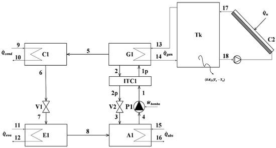
Figure 1.
Schematic diagram of the vapor absorption refrigeration cycle integrated with thermal storage tank and solar collector.
The solar collector, coupled with a thermal storage tank, is used as an energy source for the VAR cycle, as shown in Figure 1. The fluid considered for the solar assembly is water; properties such as the collector area and type of collector can be modified within the simulation, as well as the thermal tank losses and volume. The desired hour of operation of the VAR, hourly irradiation at the solar collector, and hourly variation of the room temperature can be specified as an array or vector.
The main objective of the simulation of the refrigeration cycle coupled to the solar system is to evaluate how the system will perform under user-specified conditions, so a MATLAB© App Designer application was developed in order to provide an intuitive but completed software to do so. However, the functionality of the software can be informative in educational courses such as thermodynamics or even in courses about how to develop software for engineering. A longer-term objective with software is to provide awareness. According to the International Agency of Energy (IAE), traditional refrigeration with VCR is a blind-spot in global energy politics due to the fact that as the economy grows, more VCR will be needed for better human comfort, but traditional refrigeration with VCR is slowly taking a more and more energy from the grid, causing a need for more energy, which leads to the construction of additional power plants and ultimately more greenhouse effect [22,23], which in turns increases the need of refrigeration in warm regions. This effect can be confronted by renewable technologies [24,25] and energy-saving techniques [26,27].
The software is subdivided into three phases, the first one provides a simple cycle of VAR, where no external flow is considered. This model allows a quick calculation, whose output is the power per component, the properties per state, and a TS diagram. This model is called model 1 and its validation is presented in the results section. The second model (model 2) allows a more detailed study, where there are more inputs, such as pressure drops, temperature differences, flow and temperature of external streams, cooling loads, etc., with outputs such as energy, exergy, and exergy disaggregation. Its validation is also presented in the results section. In the last stage, the coupling of model 2 with the solar array is carried out. In this stage, a case study of the irradiation and ambient temperature of the city of Barranquilla is analyzed.
2.2. Thermodynamics Analysis: Vapor Absorption Refrigeration System
Considering the mass conservation law and the steady-state consideration assumed to all components of the VAR, the mass (Equation (1)), species (Equation (2)), and energy (Equation (3)) conservation laws were applied.
Enthalpy and entropy in the states of pure water in the cycle are functions of two independent intensive properties, usually temperature and pressure, while for the states where LiBr and water are involved, the properties also depend on the water concentration in LiBr:
It is widely accepted in the analysis of this cycle that, at the output of the generator to the condenser, the refrigerant does not contain lithium bromide [6], meaning that the refrigerant is found as a stream of pure water, so:
which means that for a concentration X = 1, there is pure water, while a concentration X below 1 means that there is an amount 1 − X of LiBr in the state.
The generator, absorber, condenser, and evaporator stream outputs are considered to be in saturated condition:
Stream 2: Saturated liquid solution with a higher concentration of LiBr in water.
Stream 4: Saturated liquid solution with a lower concentration of LiBr in water.
Stream 6: Water in saturated liquid state.
Stream 8: Water in saturated vapor state.
Temperature, pressure, composition, and mass flow of the external cooling water streams supplied to the absorber and condenser, the hot fluid used as a heat source for the generator, the fluid to be cooled in the evaporator, and the cooling load are input values to the model:
Due to the extensive design possibilities, there are many considerations regarding the steam state in which the refrigerant exits the generator. For this model, we adopt the consideration presented by Wonchala et al. [28], where the generator refrigerant outlet temperature is considered to be equal to the equilibrium temperature of the weak solution:
The minimum temperature difference in the absorber, generator, condenser, and evaporator and the efficiency of the solution heat exchanger are input values:
Pressure drops by length and those due to the individual components of the absorption cooling system, with the exception of the pump and expansion valves, which are usually negligible. For the present modeling, following the recommendations presented by Morosuk and Tsatsaronis 2008 [29], the pressure drops in the generator and the absorber will be taken into account; this supports the determination of ideal, real, and inevitable operations that are useful for the disaggregation of exergy destruction:
Solution pump efficiency is defined as:
where is the outlet enthalpy of the weak solution if the pump will operate isentropically.
From the properties calculated at each point in the absorption cooling system, the system performance (COP) is defined as:
The maximum possible efficiency for an absorption cooling system (reversible COP) operating between the temperature of the heat source, the cooling fluid, and the cooled environment is defined as:
To determine the thermodynamic properties of water, it was implemented in the library of properties of CoolProp. Coolprop is a software that has an extensive database of correlations and equations needed to determine the properties of various pure and pseudo pure substances, and it is completely free-to-use [30]. CoolProp contained the properties of the LiBr–H2O solution. However, these properties did not correspond satisfactorily with the validation of different works carried out during the development of the simulation software, so it was decided to use the properties of the LiBr–H2O solution programmed manually according to the tables and correlations presented in the scientific literature.
The enthalpy h and entropy s of the LiBr–H2O solution are described by the parameters and constants resulting from the implementation of the Gibbs free energy equation on electrolyte substances by Kim and Infante for a concentration range between 0 and 70 wt% of lithium bromide in water and a temperature range between 0 and 210 °C [31].
Viscosity, concentration, density, specific heat, and conductivity were taken from the technical report of the thermophysical properties for the LiBr–H2O solution of the American Society of Heating, Refrigerating, and Air-Conditioning Engineers, ASHRAE [32].
Table 1 presents the properties of the LiBr–H2O solution, commented on before, which is attached to the admissible range of the independent input variables and literary sources where they are used:

Table 1.
Description of the properties of LiBr–H2O used.
The total flow exergy of a state, considering that potential and kinetic components are negligible, is calculated as the sum of the physical and chemical exergy:
The physical exergy of a flow is the maximum work available when the system is taken from an initial state with conditions () to a reference state () by a reversible process, exchanging energy in the form of heat and working only with the reference environment; physical exergy can be calculated using the following equation:
where h. is the enthalpy, s. is the entropy, and the sub-index zero indicates the property is in a dead state at reference temperature (T0). For water, the above equation depends on the temperature and pressure conditions, while for the LiBr–H2O solution, it also depends on the specific concentration.
The chemical exergy of a flow is the maximum work that can be achieved when the substance is brought from its equilibrium state at ambient pressure and temperature (restricted dead state) to the equilibrium state of equal chemical potential (unrestricted dead state) by a process involving heat, work, and mass transfer with the environment.
For those states where only water is present, the chemical exergy of flow is taken with a fixed value of 49.96 kJ/kg, according to [34,35]. Since the LiBr–H2O solution is not ideal, the exergy of the chemical flow for the solution is a function of the standard activities and exergies of the pure species, as represented below:
As mentioned above, Equation (23) consists of two parts, the standard chemical exergy of pure species (Equation (24)) and chemical exergy destroyed due to the dissolution process (Equation (25)):
where and represent the standard chemical exergies of water and lithium bromide, whose values are 0.9 kJ/mol and 101.6 kJ/mol, respectively.
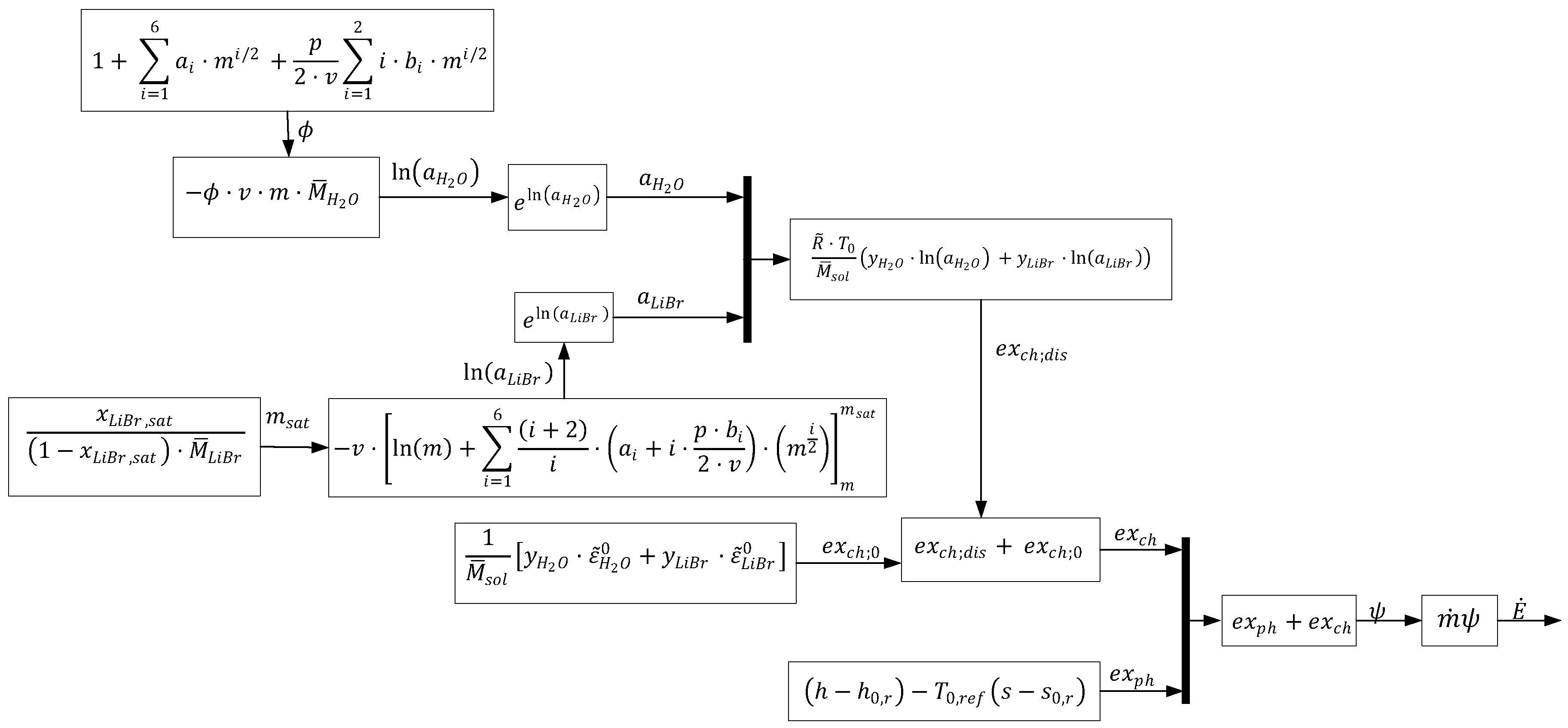
where and represent water and lithium bromide activity, respectively. A flowchart of the process to calculate the total exergy for LiBr–Water is presented in Figure 2; for a detailed explanation of each term, check [35]. After the determination and addition of both components of exergy, the total exergy expressed in terms of rate is obtained by multiplying the total flow exergy with the flow rate of that state:
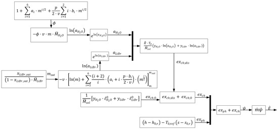
Figure 2.
Outline of exergy analysis.
The definition of fuel-product-destroyed is applied to traditional exergy analysis, where the fuel is the amount of exergy that enters a component to produce an amount of product. Similarly, the product is defined as the amount of exergy left by a component converted by the fuel that previously entered the same component. For the specific case of the component under study k, the exergy of fuel, product, and destruction is given by Equation (27).
Table 2 shows in detail the structure of fuel-product-destroyed exergy balance in each component of the absorption refrigeration system:
Table 2.
Fuel-product-destroyed structure for each component in the refrigeration cycle.
The ratio between the definitions of COPs set out by Equations (19) and (20) allows the total exergetic efficiency of the system to be defined, which represents a measure of the thermodynamic irreversibilities associated with the absorption refrigeration cycle:
Exergetic efficiency for the k component, in particular, is defined as the relationship between the produced exergy over the required exergy :
The ratio of irreversibility (IR) of each component of the absorption refrigeration cycle is defined as the ratio of exergy destroyed in the particular component and the total exergy destroyed in the system:
The exergy depletion ratio (FDR) is defined as the ratio of exergy destroyed in the particular component and the total exergy supplied to the system, in this case the exergy supplied to the generator:
2.3. Exergy Disaggregation
An exergy disaggregation allows a more detailed investigation of the cause of the exergy destruction, with the aim of identifying opportunities for improvement in each component of the system [36,37]. In order to disaggregate the irreversibilities in the absorption cooling system, the theory of advanced exergy analysis proposed by [38] is implemented, which is based on two postulates. The first proposes that the exergy destroyed can be divided into two categories according to the relevance of the component in the exergy destruction in the said component. In the first category, the exergy destruction is due to the operation of the component under consideration, which is called endogenous exergy destruction, while in the second category, there is a destruction of exergy of the component under consideration but due to the operation of the other components, which is known as exogenous exergy destruction:
Equation (32) determines whether efforts to make system improvements should focus on the component with the greatest exergy destruction, or whether the irreversibilities associated with the component with the greatest exergy destruction can be reduced more efficiently by improving operation in the other components of the cycle.
The second postulate disaggregates or categorizes the irreversibilities of the components of the cycle as avoidable and unavoidable:
Equation (33) indicates that efforts to make improvements to the system should be focused on components with appreciable avoidable irreversibilities and should not be focused on those components or processes where inevitable irreversibilities predominate.
The combined implementation of the two postulates of Equations (32) and (33) allows the destruction of exergy of the k-component to be described as:
Equation (34) highlights the fact that disaggregation into a category can be further disaggregated, resulting in four terms: is the destroyed exergy, which is due to the k-component and can be avoidable (endogenous avoidable), quantifies the destroyed exergy due to the k-component but cannot be avoidable (endogenous unavoidable), while and respectively stand for the avoidable and unavoidable destroyed exergy of the analyzed component—not due to itself but because of the interactions of other components of the cycle over this one.
The thermodynamics analysis development in the previous section features temperature differences in the condenser, evaporator, absorber, and generator as well as pressure drops in the absorber and generator (Equations (9)–(12) and Equations (14)–(17)). These configurations allow the definition of real, unavoidable, and ideal cycle conditions that allow executing the cycle with theoretical values to measure the real performance against a theoretical one. Thus, by defining real temperature differences and pressure drops, a reference model is obtained. In contrast, it is possible to define a theoretical cycle with the same characteristics as the real cycle but with no temperature difference and no pressure drop in the components, in addition to operating with isentropic turbines instead of the valves, such as the Carnot refrigeration cycle. These configurations allow the definition of ideal cycle conditions. Finally, an intermediate configuration is defined with very small temperature differences and pressure drops in the components. This configuration allows the definition of a cycle condition with unavoidable irreversibilities or the unavoidable cycle.
Following this idea, by setting real conditions and executing the vapor absorption system, exergy destroyed in each component is found. By setting unavoidable conditions and executing the cycle, the unavoidable exergy destroyed is found in each component. Establishing ideal conditions in all components while the component under analysis is established in real conditions and running the model of the refrigeration system allows finding the endogenous destroyed exergy in that component, a procedure that must be repeated in each component in order to find each endogenous destroyed exergy. In a similar way, by establishing ideal conditions in all components while the component under analysis is established in unavoidable conditions and running the model, the endogenous unavoidable destroyed exergy is found for the k-component. Again, this procedure must be repeated, setting each component to the unavoidable conditions while all others operate ideally.
Knowing , , and is enough in order to get the missing terms shown through Equations (32)–(34). By subtracting from , is found; from gives; from gives , and from gives . With these data, it is possible to make further improvement by focusing on the component of the system that has the most potentially avoidable exergy destroyed and to check whether the improvement could be achieved by focusing only on that component or on the whole cycle. This is an advantage over conventional exergy analysis, which can create motivation to improve a component that has the total exergy destroyed; however, maybe all that exergy is of an inevitable nature and, together with concepts such as thermoeconomic analysis, where each exergy destroyed is computed against a calculated cost, it can become a powerful tool for determining energy and economic improvements [39,40].
2.4. Solar Collector and Storage Tank
The model of the flat-plate solar collector is based on the equations presented by [41]. The rate of useful energy transported by the collector is defined as:
where is the useful energy collected by the solar system, is the area of the collector, is the total radiation incident on the collector, and is the instantaneous efficiency of the collector, which is defined as the ratio of useful heat over a specified period of time to the energy of the incident solar irradiation over the same period of time. Instantaneous collector efficiency is defined as:
where is the collector heat removal factor, which is calculated as the ratio of the actual rate of heat transfer to the working fluid to the actual rate of heat transfer at the minimum temperature difference between the collector absorber element and the environment; while τα is the product of transmittance−absorbance, or optical efficiency, where the transmittance is the fraction of solar incidence radiation transmitted through the collector cover, and the absorbance α is the fraction of solar incidence radiation absorbed by the collector material.
In addition, in Equation (39), is the overall transfer coefficient, is the temperature of the fluid at the collector inlet, and is the ambient temperature. Usually, the products and are characterized by a particular solar collector and dictate the performance of the collector. Their values are tabulated and obtained from experimental information in graphic form of the collector’s performance against , where is the intercept, and is the slope [41].
Data for total hourly solar irradiation is taken from metrological sources, such as the Institute of Hydrology, Meteorology and Environmental Studies (IDEAM), which have the hourly irradiation per month for different locations in Colombia for different years [42]; but, as can be seen later in the software section, the irradiation and the room temperature can be manually modified to assess the solar collector gain and therefore to assess the solar absorption system performance anywhere.
A thermal storage tank is integrated with the collection system in order to collect solar energy and provide a continuous supply of heat when solar radiation is no longer sufficient. To simplify the model, it is assumed that the water in the insulated tank is completely mixed with the water returning to the tank from the collector and generator. By performing an energy balance in the tank without stratification (i.e., completely mixed and without temperature variations lengthwise), the following equation is obtained:
where is the mass of water in the storage tank, is the calorific capacity of water, and is the ambient temperature around the tank; whereas, and represent the useful thermal energy obtained from the solar collector and the thermal energy required by the absorption cooling system (thermal load required by the generator), respectively. Additionally, represents the product coefficient that quantifies the losses per storage tank area. Its value is taken as [43]. However, it is not fixed and can be editable in the software. If , and the tank losses over a period of time ∆t are assumed to be constant, Equation (37) can be rewritten for each interval as:
where is the temperature of the storage tank at the end of that time interval , and is the temperature of the storage tank during the . At the end of each time interval , the value of obtained will be assigned as the for the next interval, and so on for the time extension of interest.
The rate of exergy absorbed from solar radiation is expressed, according to [44], as:
where represents the optical efficiency, which is equal to the transmittance–absorbance product , is the apparent temperature of the sun, which is equal to 75% of the black body temperature of the sun [45].
The definition of FDR from Equation (31) is modified to take into account the total exergy entering the system from the solar source, in the form:
2.5. LCA Solar Absorption Refrigeration System
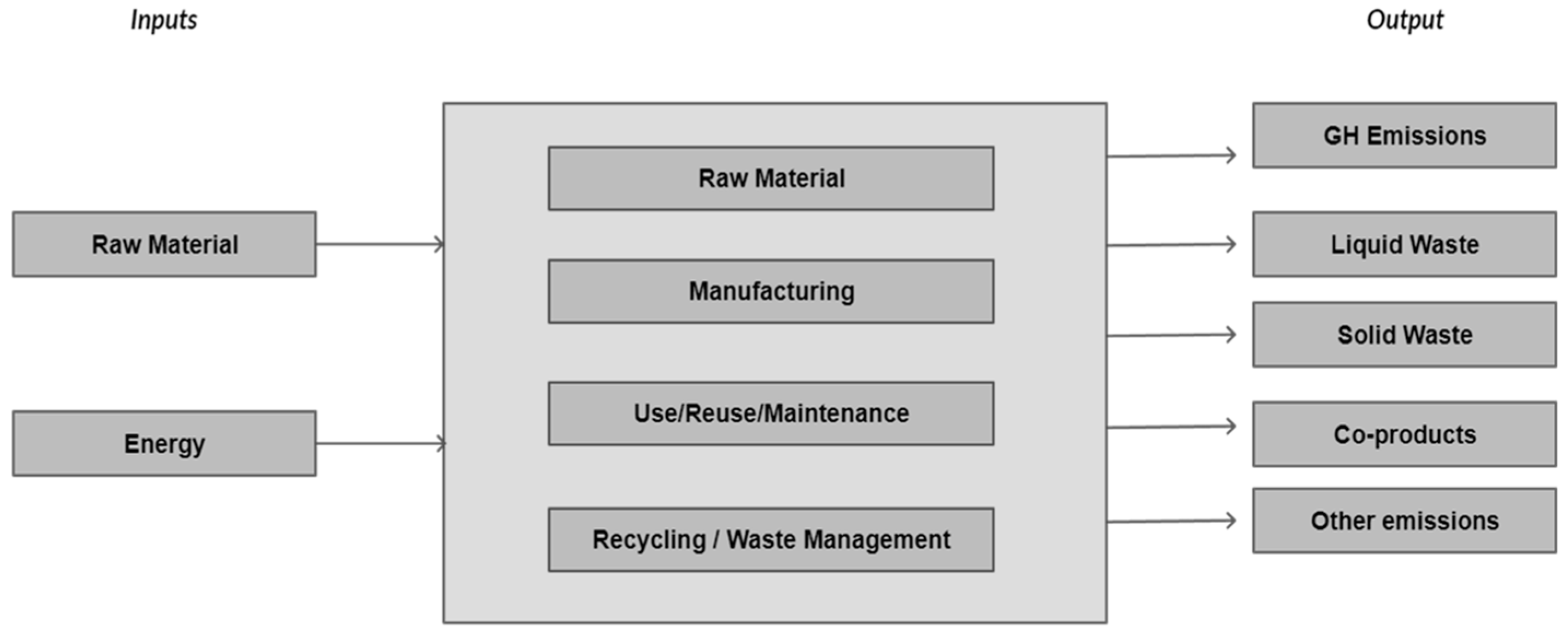
The life cycle analysis developed is a tool used for the systematic assessment of the likely environmental impacts of products, services, and technologies. This is done by examining inputs and desired emissions, wastes, and/or outputs throughout the entire product life cycle (Figure 3 and Figure 4). Through this analysis, environmental burdens are identified, and their propagation from one stage of the life cycle to another or from one environmental threat to another is prevented. The implemented LCA is a standardized method that provides an analytical basis for the evaluation and comparison of products, processes, materials, and service systems.

Figure 3.
Product Life Cycle.
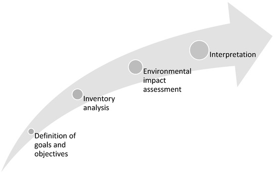
Figure 4.
Stages of an LCA.
The LCA involved the specifications of the absorption refrigeration system and compiled all relevant energy inputs, materials, and environmental releases in a quantitative inventory. The inputs and outputs of the system were evaluated taking into account the environmental impact they may have on human health, ecosystems, and resource depletion. The interpretation of these results provides further information for decision making regarding the industrial application of this equipment.
ISO 14040: 2006 [46] is used to elaborate the LCA of the solar absorption refrigeration system in four phases: definition of objective and scope, where the system boundaries and functional unit are established; inventory analysis, in which the input and output data pertaining to the product life cycle are quantified; impact assessment, which associates the inventory data with environmental impact categories; and interpretation, where the results are summarized and conclusions are drawn.
3. Results and Discussions
3.1. MATLAB App Designer Application
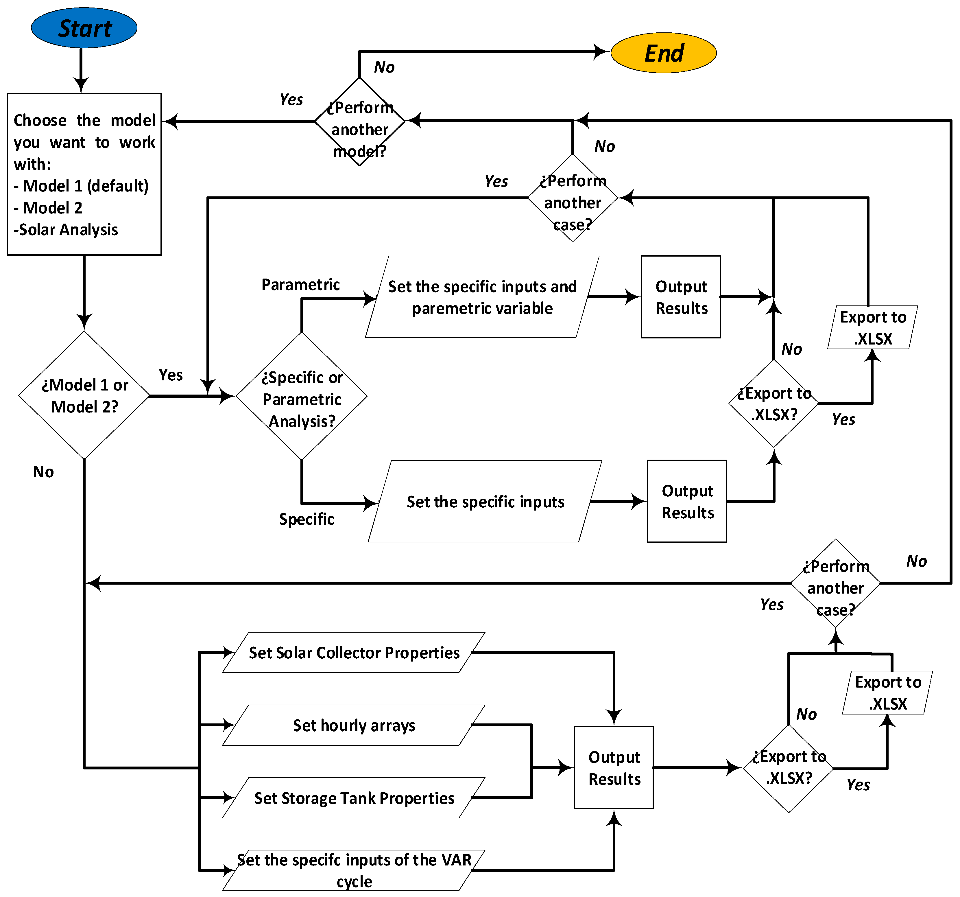
A graphical user interface was developed in MATLAB using the App Designer application for the energy, exergy, and disaggregation stages of the VAR cycle of LiBr–H2O, which consists of three tools that perform the analyses presented in the previous section. A flow chart schematic of the software is presented in Figure 5. Figure 6 shows a preview of some of the graphical user interfaces of the software packages.

Figure 5.
Software flow-chart.
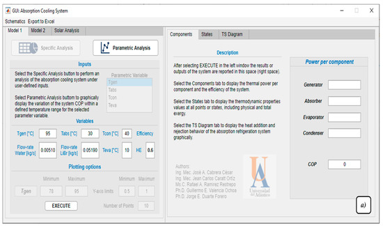
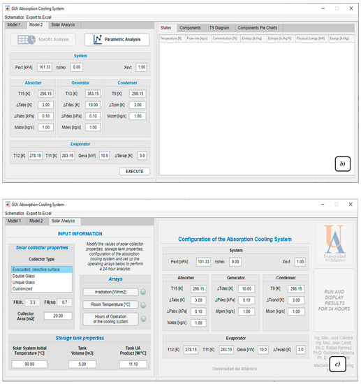
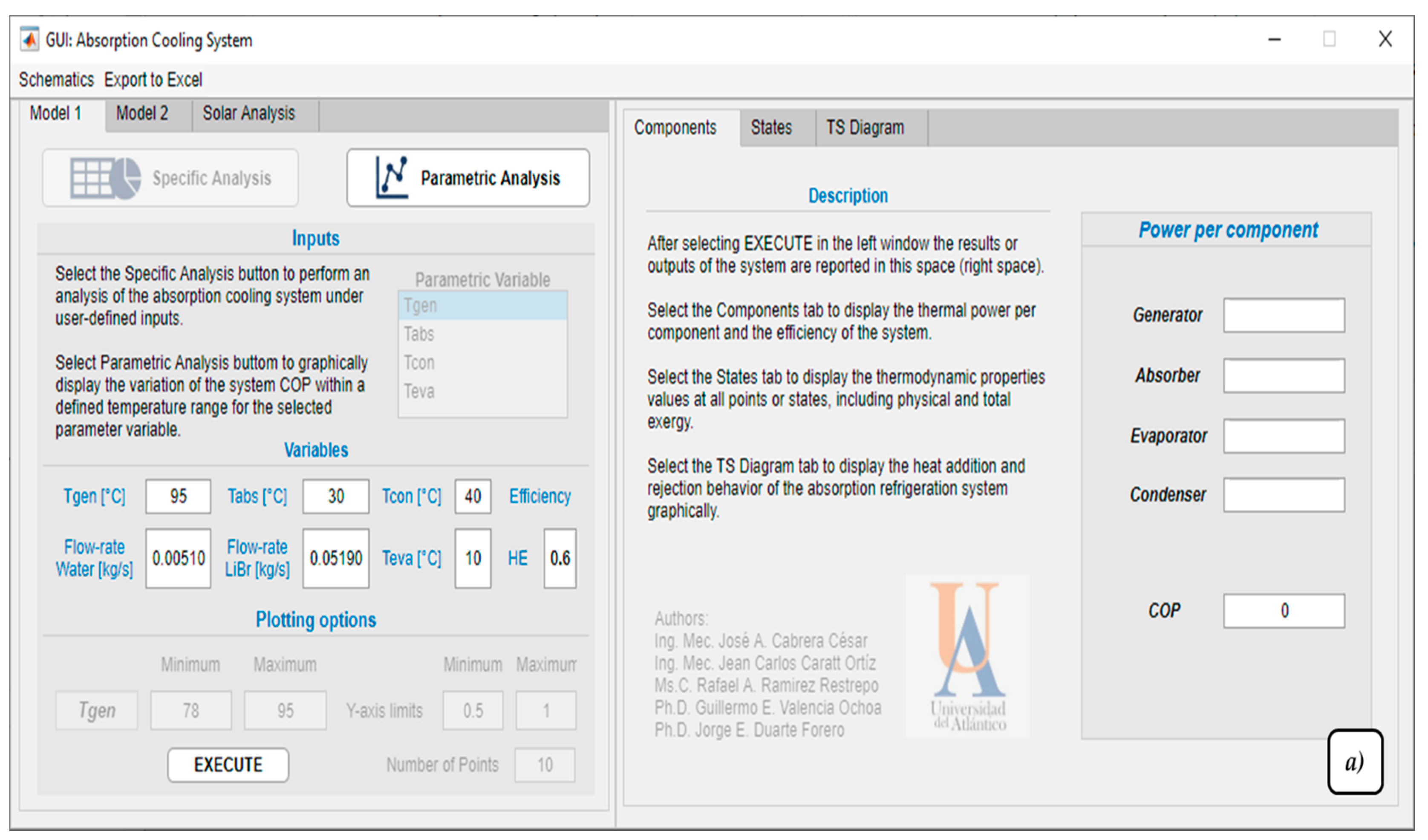
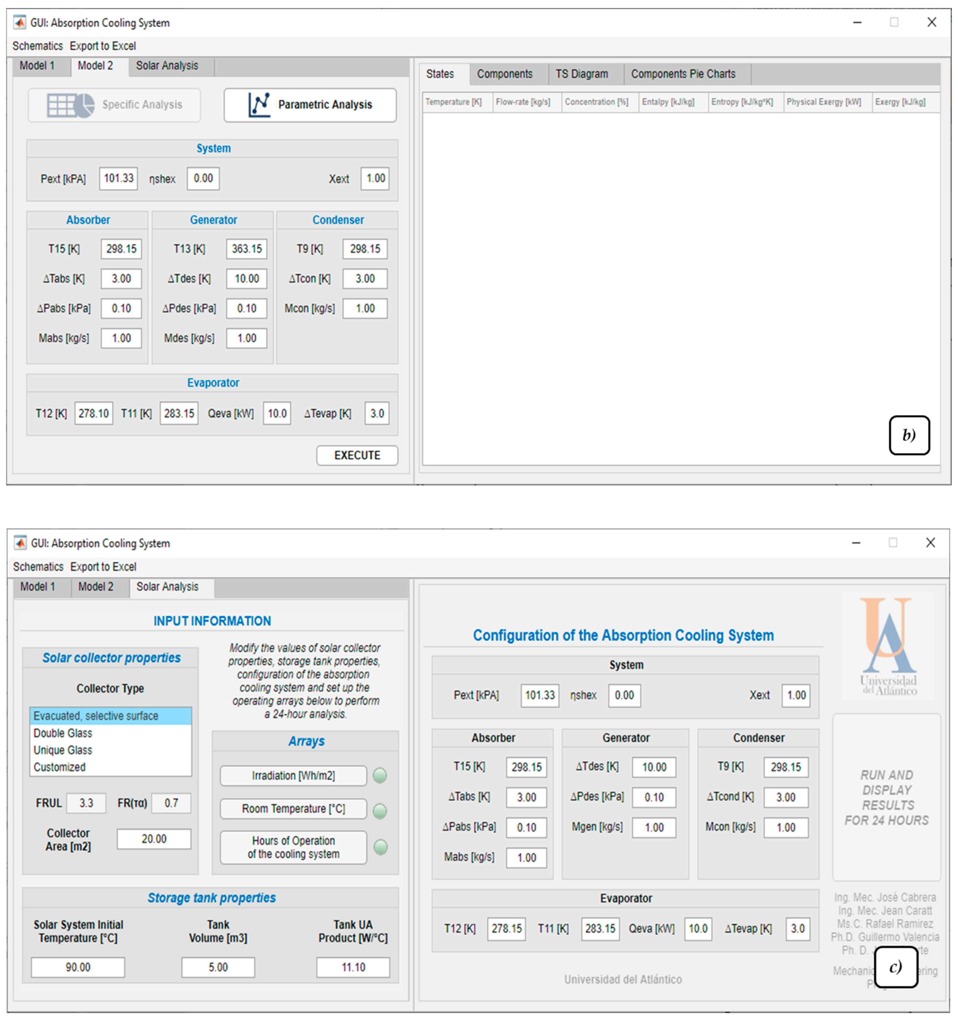
Figure 6.
Software Graphical user interface, (a) model 1 proposed, (b) model 2 proposed, and (c) solar analysis.
This software was registered with the number 13-79-348 in the DNDA. In order to execute the program, it is necessary to have already installed MATLAB Runtime and Coolprop in the default folder and Windows operating system with a least 100 Mb of free space on the local disk.
Model 1 (Figure 6a) allows validation of the LiBr–H2O single-effect absorption refrigeration system for basic conditions, i.e., when only information about the temperature of the four internal components, mass flows, and heat exchanger efficiency is presented. It is important to note that the number of models and considerations presented in the literature for this system is vast, so the results may differ from one particular study to another. Since the model does not include external streams, the energy and exergy capacity of the calculation is limited to providing the values of the thermal power used by the components, the properties by states of the system, and a temperature-entropy diagram of the system. The development of this model is based on the study presented by [47]. This model has a Specific Analysis mode, where detailed results are presented, and a Parametric Analysis mode, where it is possible to vary the temperature of a particular component and see its impact on the performance variable for this particular model, COP.
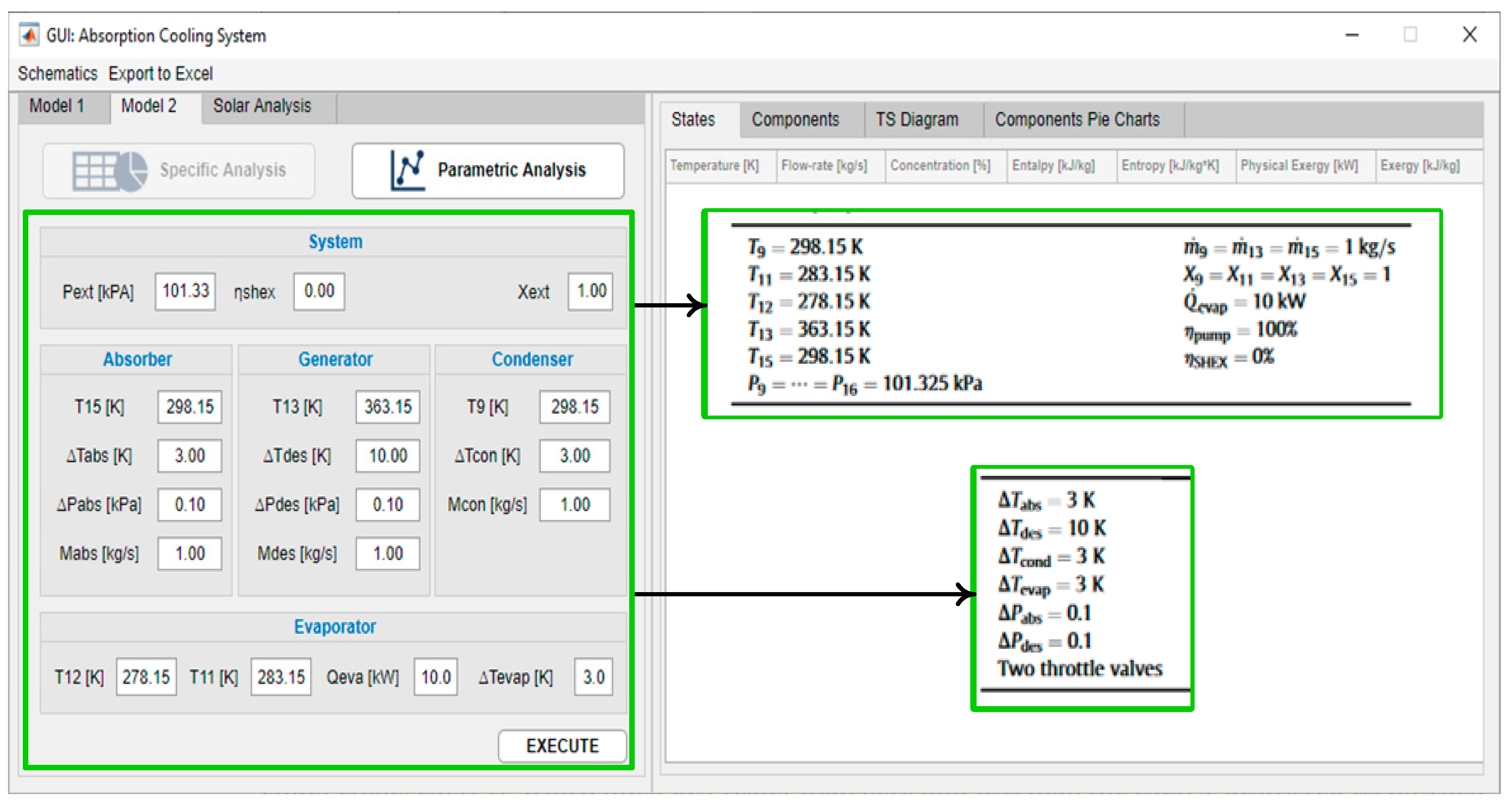
The second tool or model 2 (Figure 6b) allows a complete energy and exergy analysis of the absorption cooling system to be performed, to the point of being able to break down the destroyed exergy of the components into four types (endogenous, exogenous, avoidable, and unavoidable) by implementing the real, ideal, and unavoidable conditions due to pressure drops and temperature differences in the same components, as well as taking into account the effect of external streams over the characteristic components of the LiBr–H2O single-effect absorption cooling system. This tool also features specific analysis for detailed performance information for fixed conditions and parametric analysis for conditions where external streams temperatures vary. The modeling of this tool is based on the model presented [33,34].
The third tool or solar analysis (Figure 6c) allows a dimensioning of a solar collection system composed of a thermal storage tank and a solar collector coupled with a LiBr–H2O absorption cooling system similar to the one presented in model 2. The tool simulates operation over a 24 h period, where the storage tank will supply temperature to the cooling system as if it were a thermal battery. The tool allows indication of whether the cooling system operates continuously or is turned on for a particular period of time, simulating a more appropriate and conscious use of the system. It is important to note that, due to the nature of change, the utility of the tool can be interpreted as a model in a transient state. However, the model actually applies a stationary operation at each hourly interval, so the properties during one hour of execution will not change until the next hour begins.
3.2. Properties Validation
For the development of the software, correlations from different sources were used, as shown in Table 1, referring to the LiBr–H2O. It is of interest to validate the accuracy of these properties since the thermal properties are a function of the type of model used by each author and since different thermodynamic modeling approaches have been found for absorption cooling systems [6,48].
Due the clear explanation of thermodynamical modelling of Gong and Boulama [49] and Wonchola [28], their model was adopted; however, as mentioned, the thermal properties are taken from different sources, so the aim of this section is to validate such properties in the particular case presented in [49,50]. Table 3 presents a comparison regarding the flow-rate, concentration of LiBr, and temperature, while Table 4 presents pressure, enthalpy, and entropy; the maximum relative error found was of 2.65% for two states referring to enthalpy, followed by 1.61% for two states of entropy and 1.45% for two states of flow-rate.
Table 3.
Fuel-product-destroyed structure for each component in the refrigeration cycle.
Table 4.
Fuel-product-destroyed structure for each component in the refrigeration cycle.
3.3. Software Validation
The tab of tool number 1 was validated with the article by [47]; in Figure 7, it can be seen how the performance of a system with two temperature conditions for the absorber can be replicated while varying the temperature of the generator.
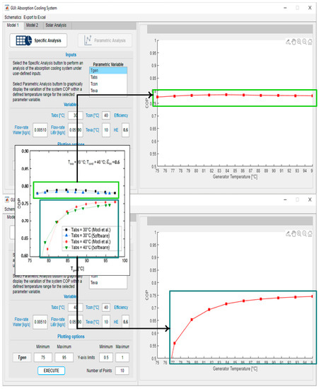
Figure 7.
Software user interface, model 1.
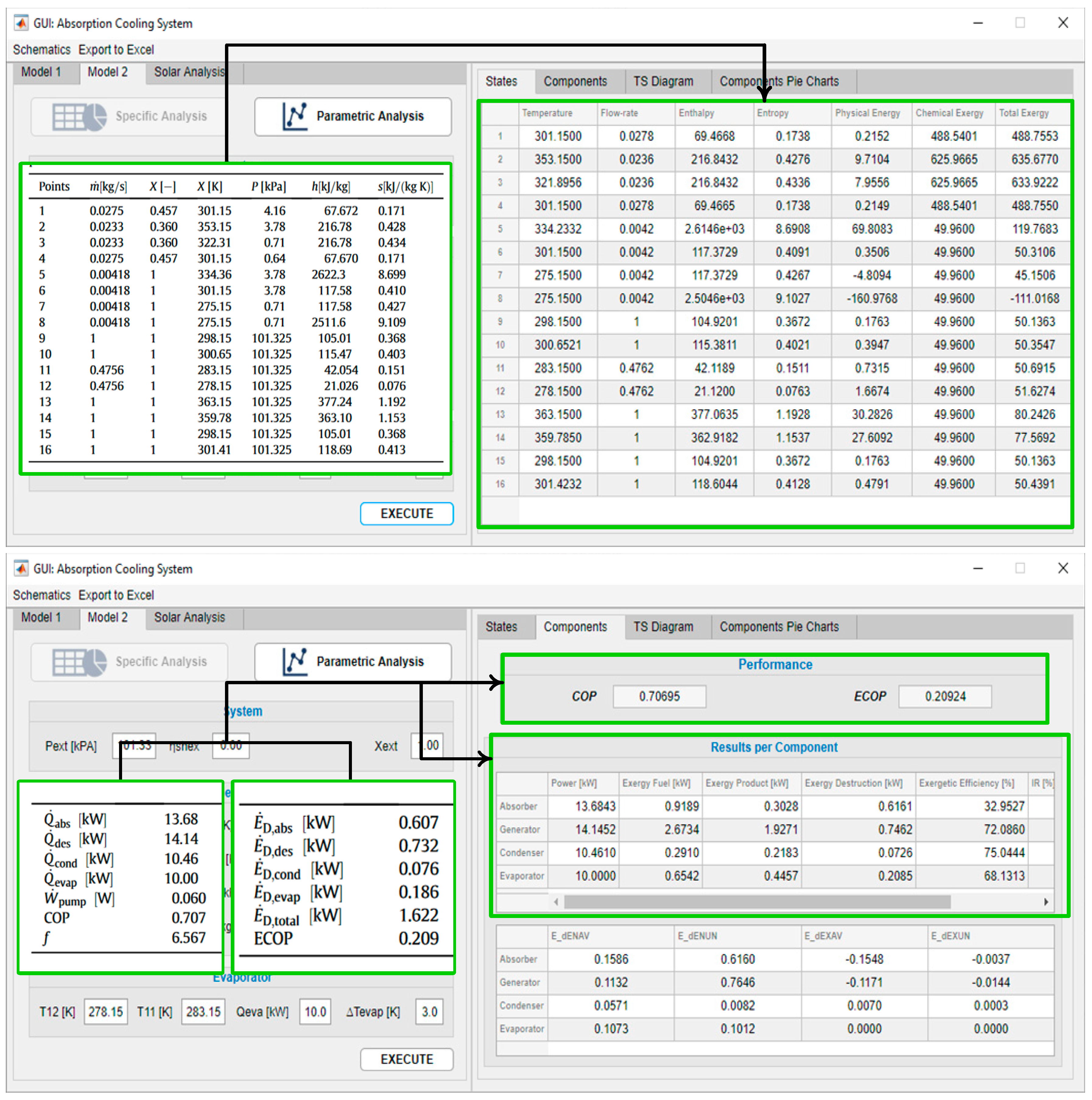
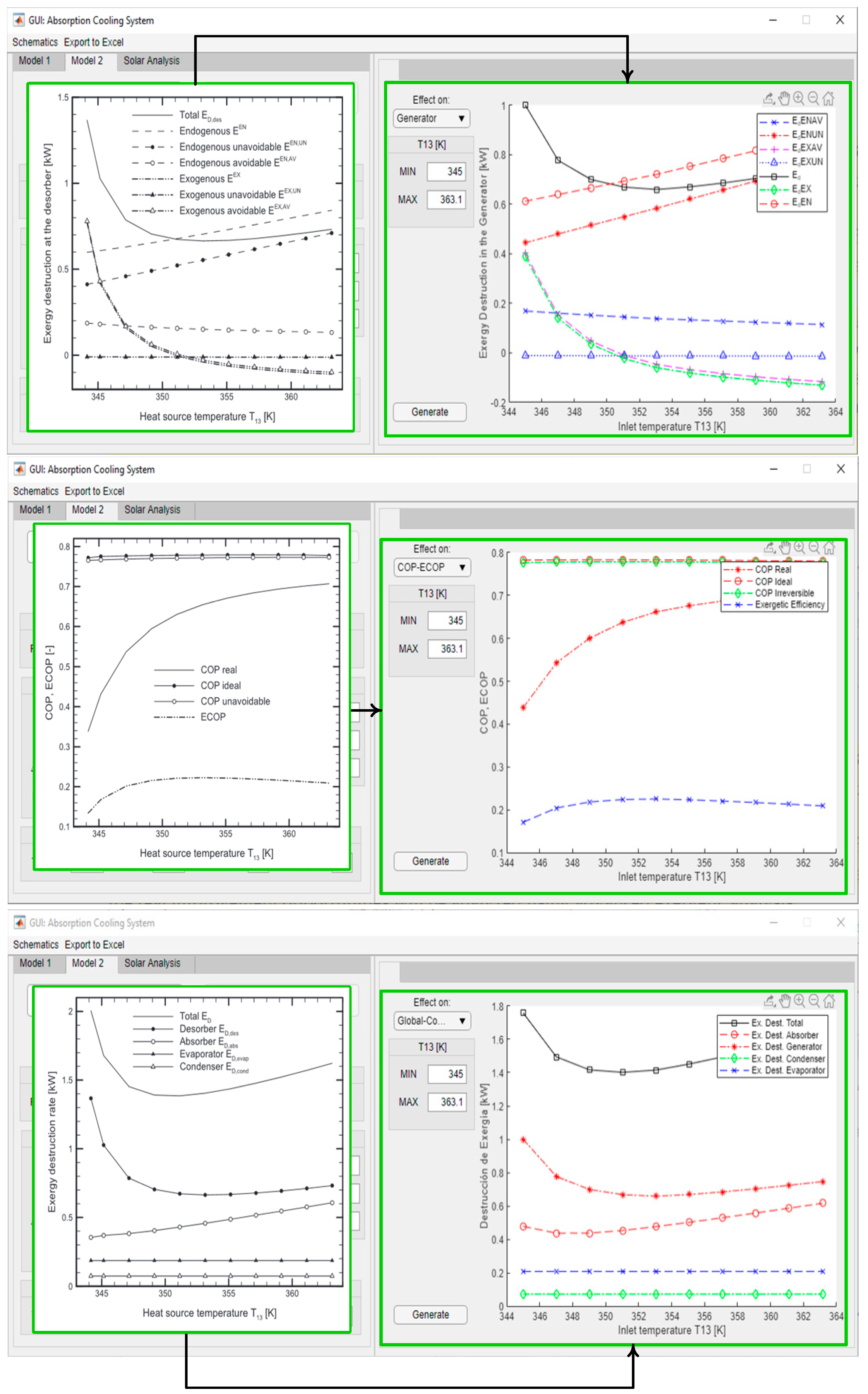
The second tool of the program was validated with [49]. Figure 8 shows how the same input conditions, reported in Gong’s system, are established in the software. Figure 9 shows the properties’ outputs per state and the energy and exergy per component of the tool against the results reported by Gong. Figure 10 corresponds to the output of the parametric analysis option, where one can see the effect of the temperature variation of one component on another or on the global system, taking as a reference the performance, exergy efficiency, total exergy destroyed, or its disaggregation by component.
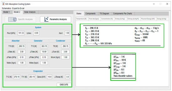
Figure 8.
Software user interface, model 2.
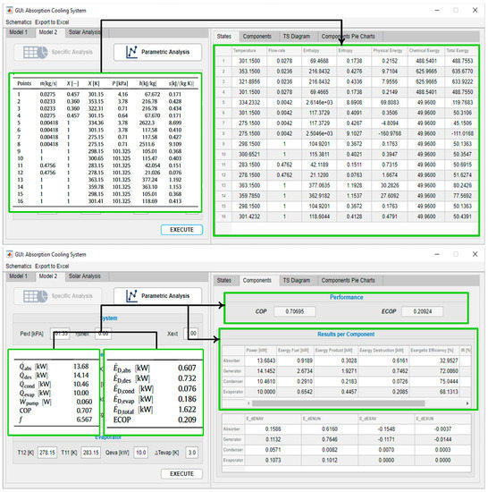
Figure 9.
Results, model 2.
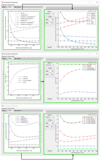
Figure 10.
Results, model 2.
3.4. Solar Analysis
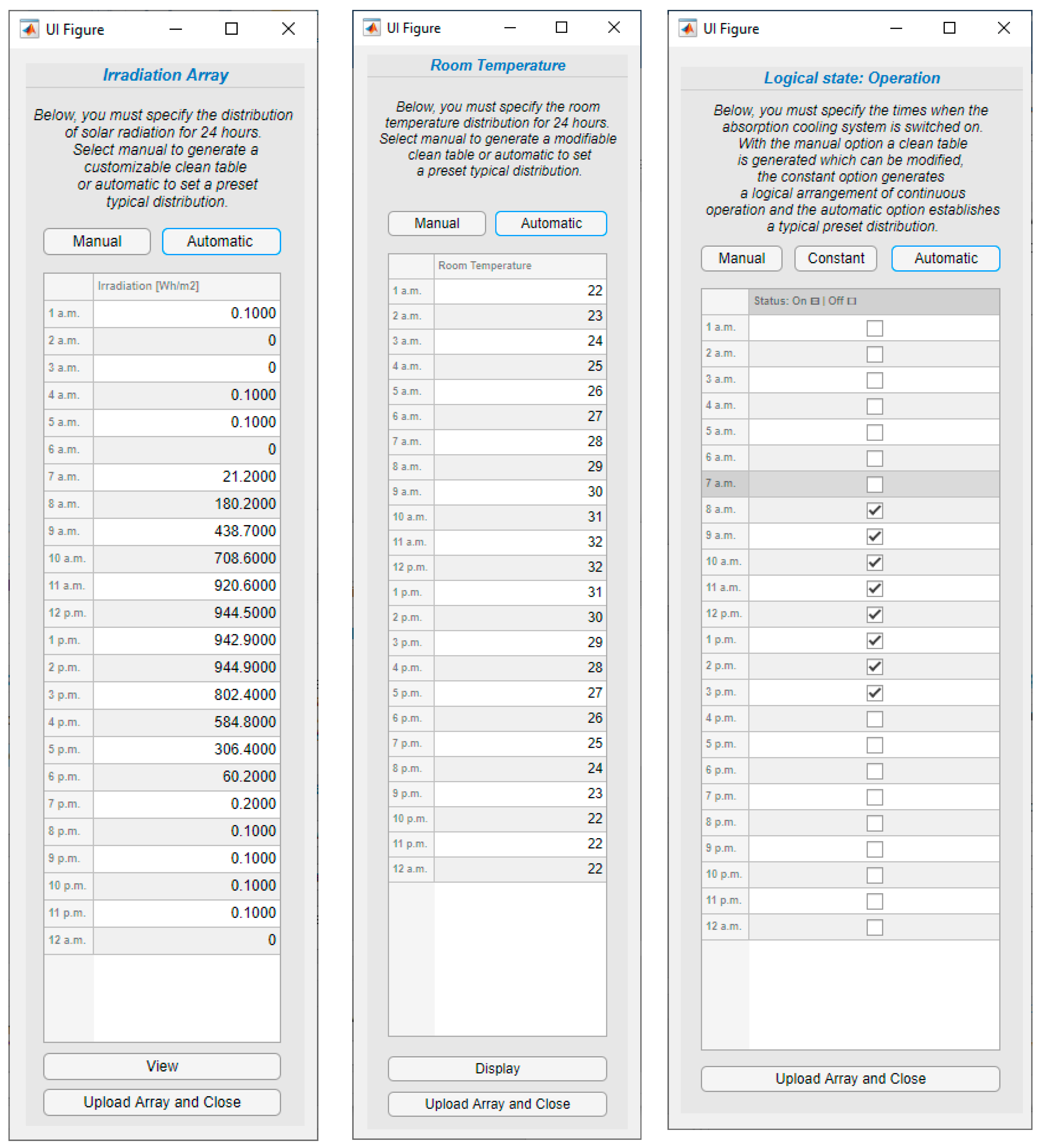
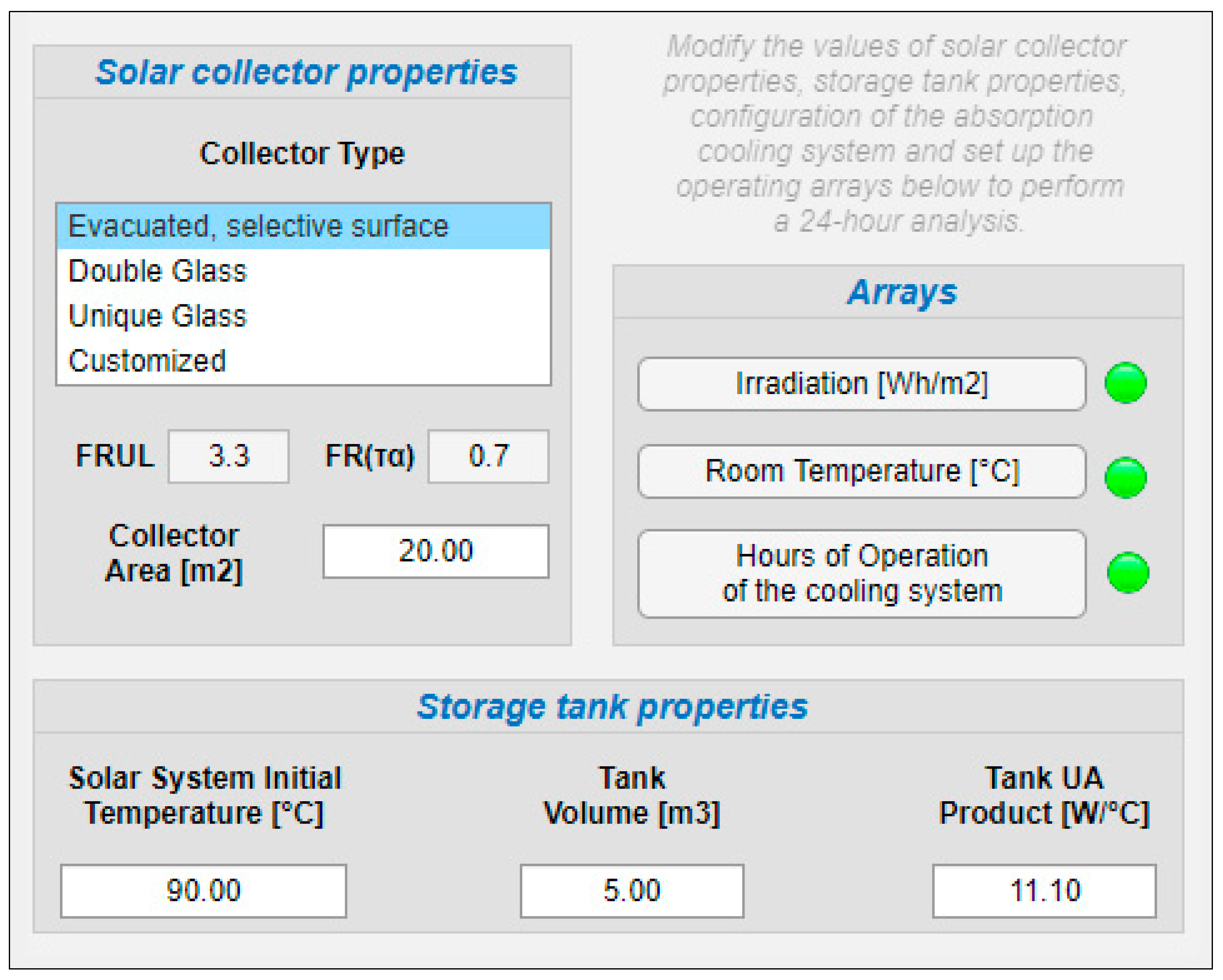
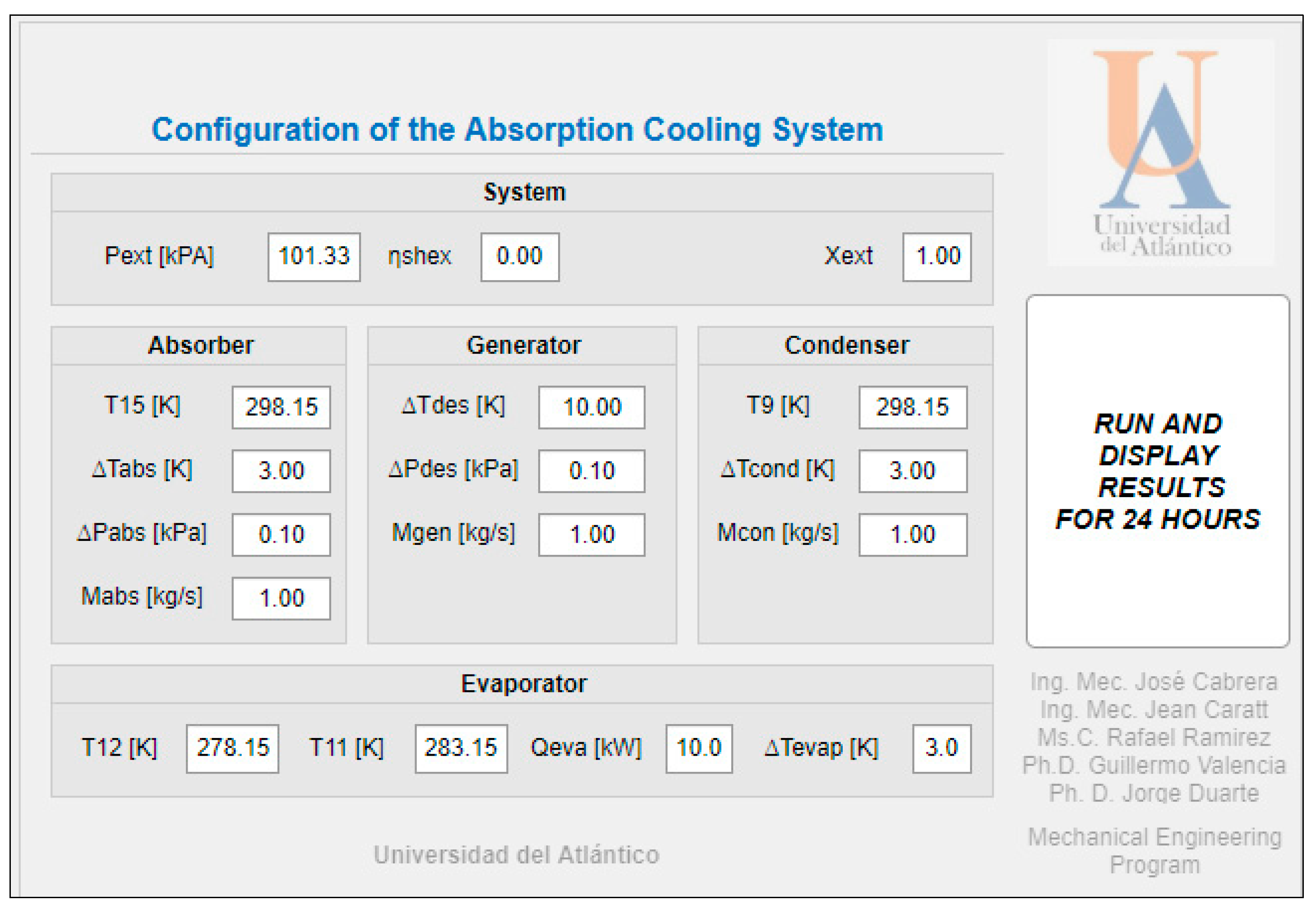
The last software tool allows making a solar analysis of the absorption cooling system for a period of 24 h of operation by entering information similar to model 2. For this purpose, the hourly array configuration is presented in Figure 11, the solar collector and storage tank configuration are presented in Figure 12, and the VAR configuration in Figure 13.
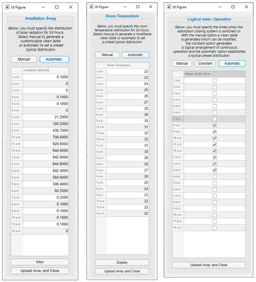
Figure 11.
Operation array values.
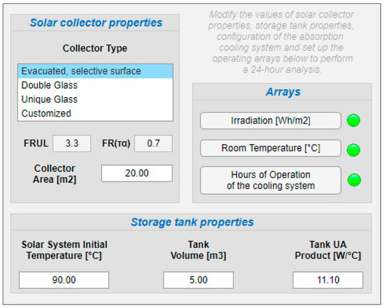
Figure 12.
Solar collector and storage tank properties.
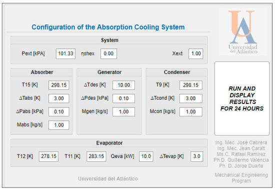
Figure 13.
VAR cycle configuration for the solar assembly.
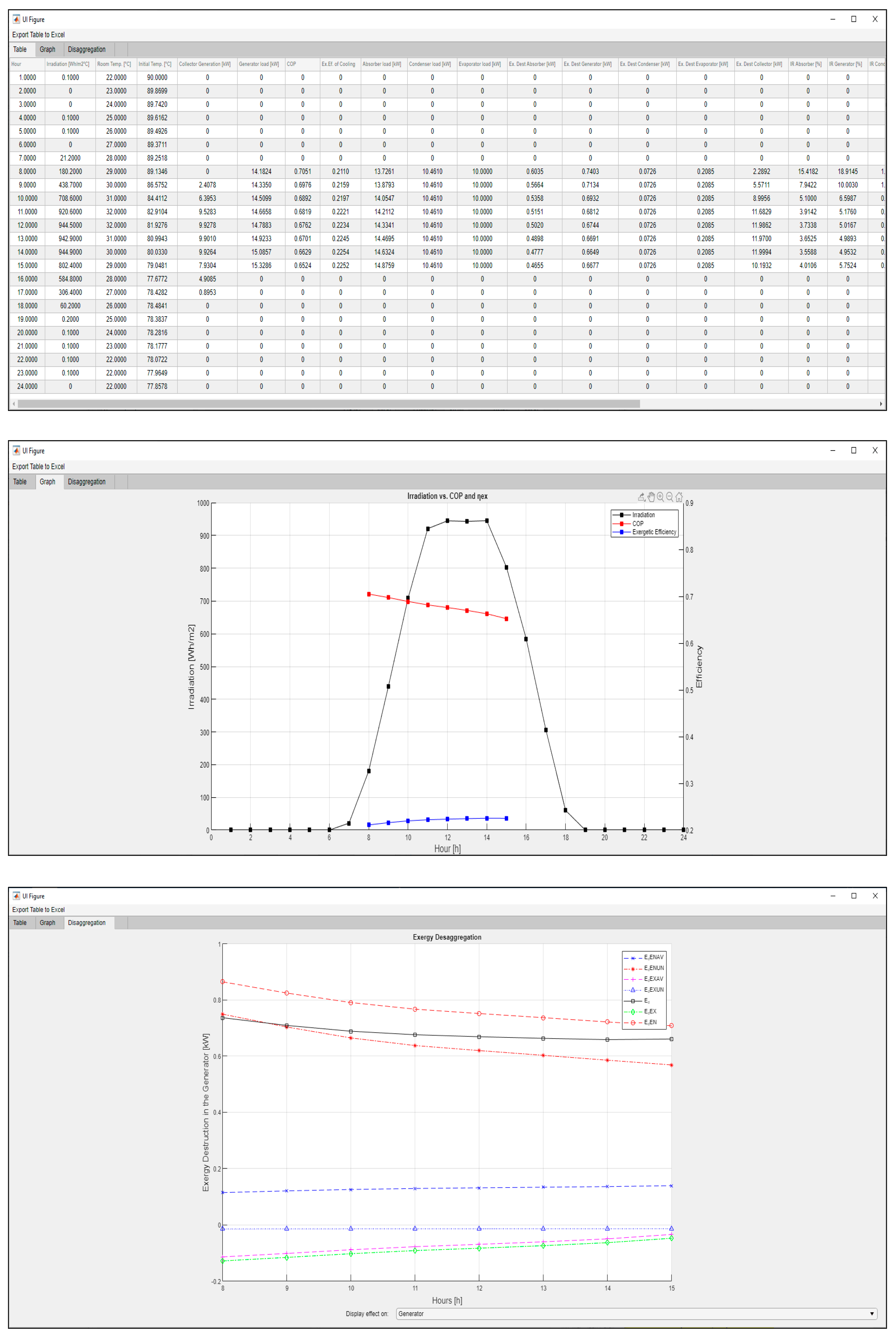
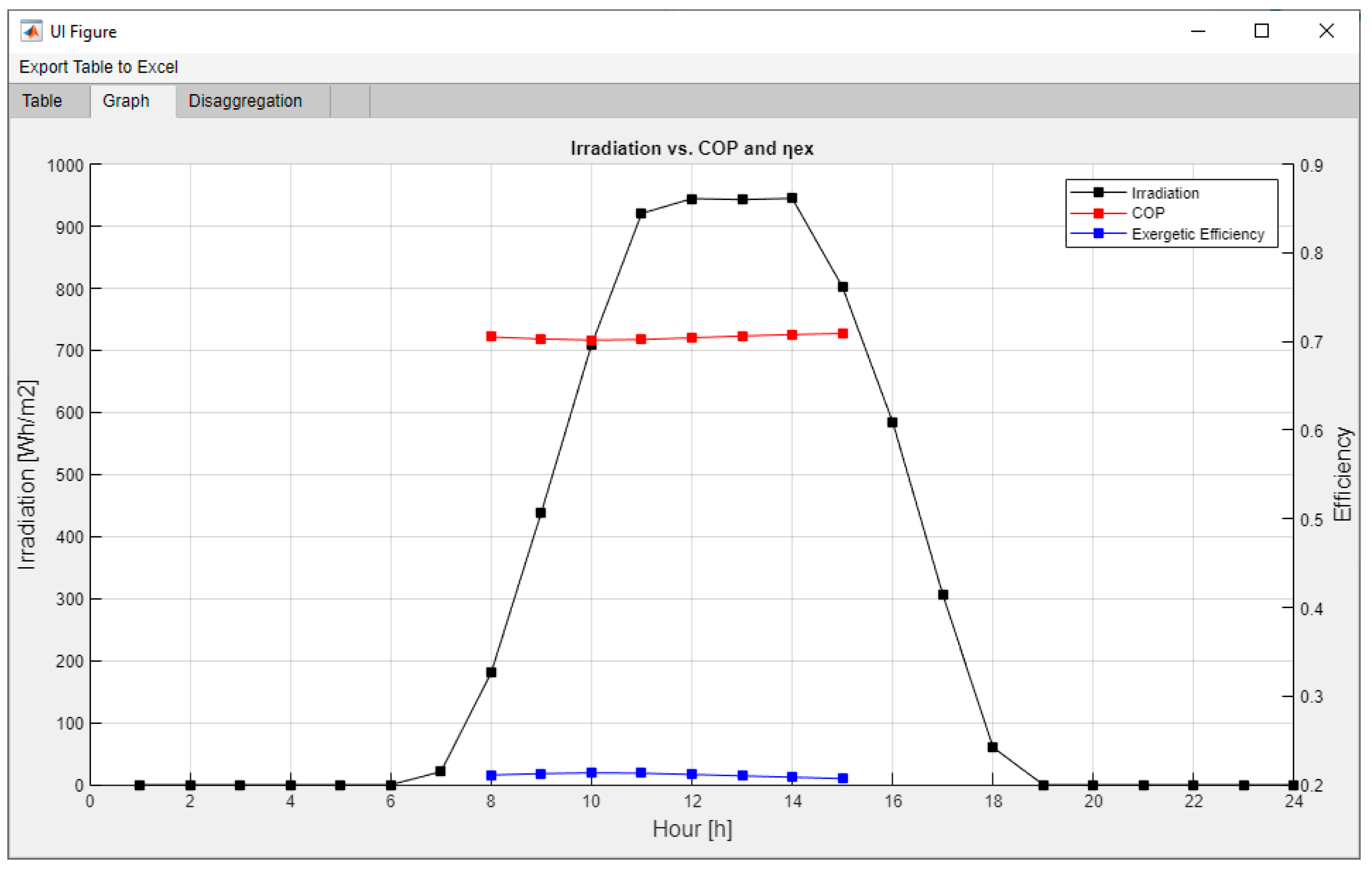
As can be seen in Figure 14, a large dataset is generated for each hour of operation for the coupled system, including the collector generation, each component’s power, exergy destroyed, irreversibility ratio (IR), and exergy depletion ratio (FDR), along with a plot solar irradiance per hour against COP and exergy efficiency, and finally, parametrical plots of the exergy disaggregation in the selected component for each hour of operation previously defined in the logical state of operation.
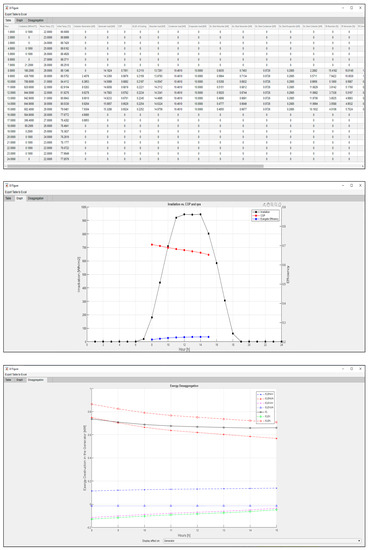
Figure 14.
VAR cycle coupled with the solar assembly outputs.
This particular case indicates that when the VAR system is turned up for high-temperature hours, the solar irradiance will not be enough to keep a stable temperature in the storage tank water, and therefore the thermal quality of water exchanging heat with the generator will drop slowly, causing the need of more thermal power for the fixed cooling load required of 10 kW. This case can be easily resolved by implementing an electrical resistance as a way to supply the temperature difference to guarantee a stable cooling supply without variation of thermal power in the generator. However, this would make outdated the energy and exergy output of the model since it would always be the same and could just be modeled by model 1 or model 2, while the only new unknown to solve would be the power needed to supply in each case due to the electrical resistance. Executing a different scenario, shown in Figure 15, the same model but with a 3.33 kW of required cooling load, gives a more stable performance in the VAR.
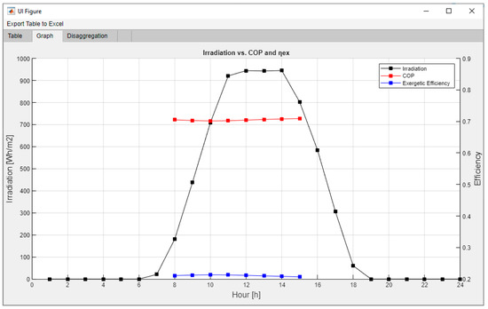
Figure 15.
VAR cycle coupled with the solar assembly outputs.
3.5. LCA Solar Absorption Refrigeration System Results
The contribution to the climate change impact category is mainly due to the CO2 emissions generated in the construction process of the refrigeration system equipment, more specifically in the steel used. The results of the life cycle analysis in the evaluated case of the solar absorption refrigeration system show that the largest generator of potential emissions that impact climate change is the energy used in the equipment where unit operations occur, such as heat exchangers, contributing 48.1% of total emissions by the energy line used.
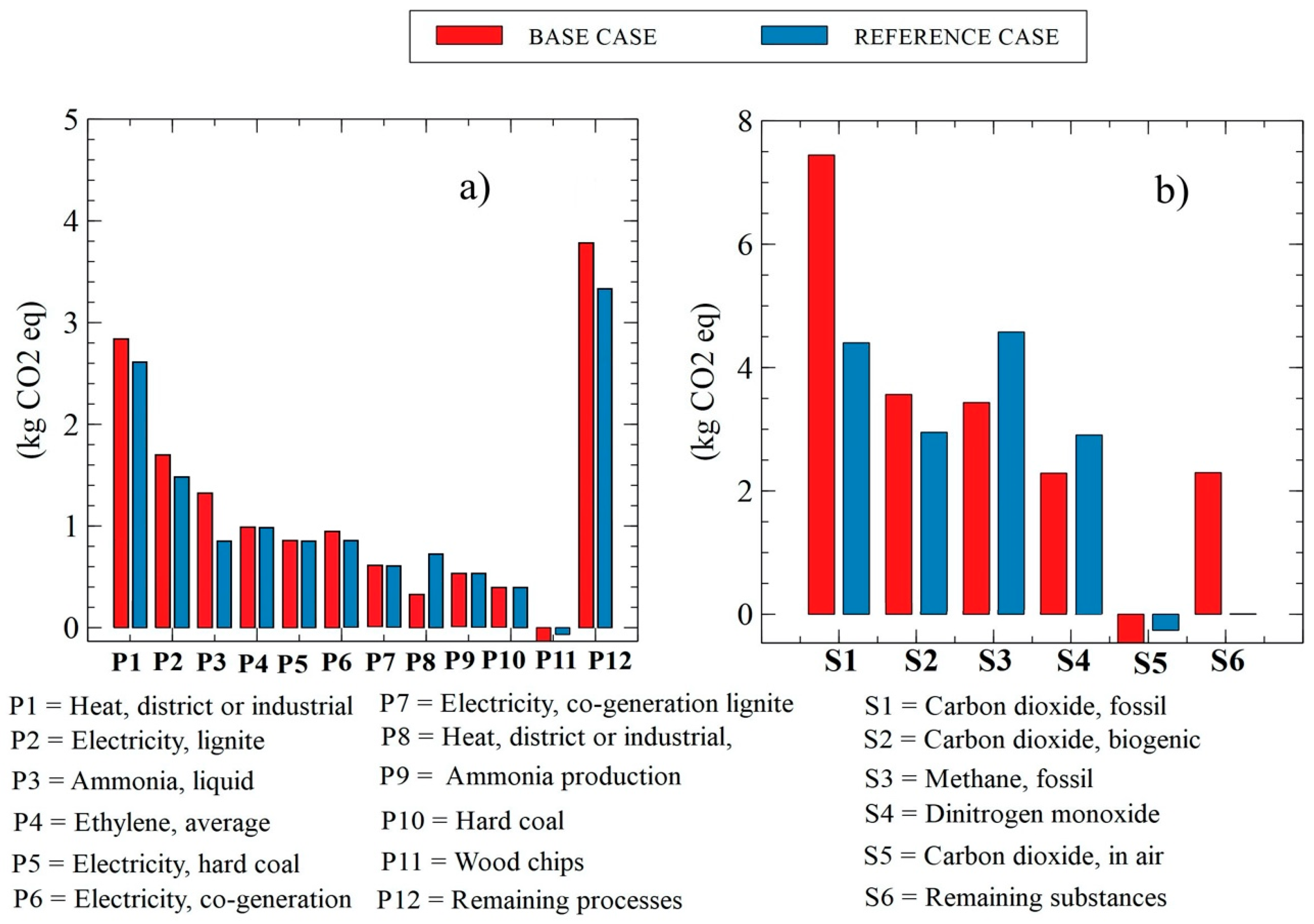
Figure 16 shows the results of the evaluated inventory, thus allowing us to observe the potential kg of CO2 equivalents that are sent to the environment throughout the entire life cycle. These results are established by processes (Figure 16a) and substances (Figure 16b) that are involved in this category.

Figure 16.
Environmental impact in kg of potential CO2 equivalents emitted by (a) processes and (b) substances.
Figure 16a shows the kg of CO2 equivalent potential emitted by the processes, showing that the base case of the plant evaluated in this study emits 1 kg of CO2 more per kg processed than the reference plant for this study due to the processes that are cogenerated with the production of thermal energy through solar energy, which shows the characteristics of the resources used in this type of refrigeration equipment. In the analysis of the impacts generated by the substances as shown in Figure 16b, it can be observed that the carbon dioxide emitted into the atmosphere by the use of fossil fuels emits approximately 4.4 kg of CO2 equivalent more than the reference plant used by the SimaPro® database, showing the inefficiencies of the processes that are generated by the equipment used in the process. In addition, we can observe that there are fields such as P11 and S5 where negative values in emissions are generated, which is due to the fact that in the process of converting solar energy to thermal energy through these systems, these processes and substances have no impact on the category of climate change because no emissions are generated.
4. Conclusions
A computational tool that allows simulating a vapor absorption refrigeration system was created through the use of a new MATLAB GUI application, App Designer. A reliable accuracy was obtained in the context of previously published research, although using different properties for the lithium bromide–water solution. This software can be executed as a standalone application. Its developed aims are to help the implementation of a new renewable system in the Caribbean Colombian zone, especially a renewable system that is fueled by solar energy because the Caribbean region benefits from high solar irradiance.
The software shows a good correspondence when calculating the energy, exergy, and advanced exergy components for the particular set of inputs proposed by Gong and Boulama [49] and Wonchala [28]. A solar harvesting system model was coupled to the vapor absorption refrigeration system, and under the user-defined ambient temperature, irradiance, and hours of working vectors, it is possible to visualize how such a system would work under 24 h of operation.
Due to the lack technical and theoretical knowledge, vapor absorption refrigeration (VARs) systems coupled with solar assembly have not been widely taken into account as a possible air conditioning solution in those regions where there is a good solar irradiance. In addition, due to the same reasons, there are not many manufactures and local industries; however, it seems that this situation will only last for a few more years because countries from Europe and Asia have been promoting such technologies, achieving a good impact in national industry and among domestic customers. It is the right time for this technology to be adopted in the Americas and specifically in the Caribbean area, where there is high solar irradiation that can be usefully employed in this system and where clean energy production can ultimately benefit human comfort.
Author Contributions
Conceptualization: G.V.O., J.R.N.A. and R.R.R.; methodology: J.C.C. and J.C.O.; software: J.C.C. and J.C.O.; validation: J.C.C. and J.C.O.; formal analysis: J.C.C. and J.C.O.; investigation: G.V.O., J.R.N.A. and R.R.R.; resources: G.V.O., J.R.N.A. and R.R.R.; writing—original draft preparation: J.C.C. and J.C.O.; writing—review and editing: G.V.O., J.R.N.A. and R.R.R.; funding acquisition: G.V.O., J.R.N.A. and R.R.R. All authors have read and agreed to the published version of the manuscript.
Funding
This work was supported by Vicerrectoría de Investigaciones, Extensión y Proyección Social from the Universidad del Atlántico, with the grand 002849 of 7 October 2020.
Institutional Review Board Statement
Not applicable.
Informed Consent Statement
Not applicable.
Acknowledgments
The authors are very thankful to the Universidad del Atlántico through the Program for Strengthening the Quality of Scientific Publications and the Visibility of Research organized by Vicerrectoría de Investigaciones, Extensión y Proyección Social. This research was supported by the Mechanical Engineering Program of Universidad del Atlántico. The Kai Research Group supports G. Valencia and J. Cabrera, and the Dimer Research Group supports R. Ramirez and J. Caratt.
Conflicts of Interest
The authors declare no conflict of interest.
Abbreviations
The following abbreviations are used in this manuscript:
| IDEAM | Institute of Hydrology, Meteorology and Environmental Studies (in Spanish: Instituto de Hidrología, Meteorología y Estudios Ambientales) |
| VCR | Vapor compression refrigeration |
| VAR | Vapor absorption refrigeration |
| COP | Coefficient of performance |
| ECOP | Exergy efficiency |
| IR | Ratio of irreversibility |
| FDR | Exergy depletion ratio |
| HCFC | hydrochlorofluorocarbons |
| IAE | International Agency of Energy |
| ASHRAE | American Society of Heating, Refrigerating, and Air-Conditioning Engineers |
| LCA | Life cycle analysis |
| GUI | Graphical user interface |
| Nomenclature | |
| Exergy flow (kJ/kg) | |
| Total exergy (kW) | |
| Exergy efficiency (%) | |
| Mass flow rate (kg/s) | |
| Mass (kg) | |
| Heat transfer (kW) | |
| Temperature (K) | |
| Pressure (kPa) | |
| Pressure drop (kPa) | |
| LiBr–water concentration (%) | |
| Useful power produced by solar collector (kW) | |
| Solar collector area (m2) | |
| Total solar irradiance incident on the solar collector (Wh/m2) | |
| Instantaneous efficiency of the solar collector (%) | |
| Solar collector heat removal factor (dimensionless) | |
| Transmittance–absorbance product or optical efficiency (%) | |
| Thermal power required by VAR (kW) | |
| Product coefficient of losses per storage tank area (W/°C) | |
| interval (°C) | |
| Temperature of the storage tank during the next interval (°C) | |
| Room temperature (°C) | |
| Apparent temperature of the Sun (°C) | |
| Calorific capacity (J/K) | |
| in | Input |
| out | Output |
| Superscripts | |
| AV | Avoidable |
| UN | Unavoidable |
| EN | Endogenous |
| EX | Exogenous |
| EN, AV | Endogenous avoidable |
| EN, UN | Endogenous unavoidable |
| EX, AV | Exogenous avoidable |
| EX, UN | Exogenous unavoidable |
| Subscripts | |
| s | Systems/plural |
| rev | Reversible cycle |
| Physical | |
| Chemical | |
| Saturated | |
| Absorber | |
| Generator | |
| Condenser | |
| Evaporator | |
| Solution heat exchanger | |
| Solution | |
| Indicates the property is in reference conditions. | |
| K-th component | |
| Fuel of K-th component | |
| Product of K-th component | |
| Destruction of K-th component | |
| Standard chemical property of pure species | |
| Chemical property destroyed due to the dissolution process | |
References
- Solano–Olivares, K.; Romero, R.J.; Santoyo, E.; Herrera, I.; Galindo–Luna, Y.R.; Rodríguez–Martínez, A.; Santoyo-Castelazo, E.; Cerezo, J. Life cycle assessment of a solar absorption air-conditioning system. J. Clean. Prod. 2019, 240, 118206. [Google Scholar] [CrossRef]
- Khan, J.; Arsalan, M.H. Solar power technologies for sustainable electricity generation—A review. Renew. Sustain. Energy Rev. 2016, 55, 414–425. [Google Scholar] [CrossRef]
- Alobaid, M.; Hughes, B.; Calautit, J.K.; O’Connor, D.; Heyes, A. A review of solar driven absorption cooling with photovoltaic thermal systems. Renew. Sustain. Energy Rev. 2017, 76, 728–742. [Google Scholar] [CrossRef] [Green Version]
- Shirmohammadi, R.; Soltanieh, M.; Romeo, L.M. Thermoeconomic analysis and optimization of post-combustion CO2 recovery unit utilizing absorption refrigeration system for a natural-gas-fired power plant. Environ. Prog. Sustain. Energy 2018, 37, 1075–1084. [Google Scholar] [CrossRef]
- Salmi, W.; Vanttola, J.; Elg, M.; Kuosa, M.; Lahdelma, R. Using waste heat of ship as energy source for an absorption refrigeration system. Appl. Therm. Eng. 2017, 115, 501–516. [Google Scholar] [CrossRef]
- Herold, K.E.; Radermacher, R.; Klein, S.A. Absorption Chillers and Heat Pumps; CRC Press: Boca Raton, FL, USA, 2016; ISBN 9781498714358. [Google Scholar]
- Mendoza, E.; Velásquez, M.; Medina, D.; Nuñez, J.R.; Grimaldo, J.W. An analysis of electricity generation with renewable resources in Germany. Int. J. Energy Econ. Policy 2020, 10, 361–367. [Google Scholar] [CrossRef]
- Nuñez, J.R.; Benitez, I.; Llosas, Y. Communications in Flexible Supervisor for Laboratory Research in Renewable Energy. IOP Conf. Ser. Mater. Sci. Eng. 2020, 844, 012016. [Google Scholar] [CrossRef]
- Gao, J.T.; Xu, Z.Y.; Chiu, J.N.W.; Su, C.; Wang, R.Z. Feasibility and economic analysis of solution transportation absorption system for long-distance thermal transportation under low ambient temperature. Energy Convers. Manag. 2019, 196, 793–806. [Google Scholar] [CrossRef]
- Núñez Alvarez, J.R.; Benítez, I.F.; Proenza, R.; Luis, V.S.; David, D.M. Metodología de diagnóstico de fallos para sistemas fotovoltaicos de conexión a red. Rev. Iberoam. Autom. Inf. Ind. 2020, 17, 94–105. [Google Scholar] [CrossRef]
- Ansarinasab, H.; Hajabdollahi, H.; Fatimah, M. Life cycle assessment (LCA) of a novel geothermal-based multigeneration system using LNG cold energy- integration of Kalina cycle, stirling engine, desalination unit and magnetic refrigeration system. Energy 2021, 231, 120888. [Google Scholar] [CrossRef]
- Murphy, M.P.A. COVID-19 and emergency eLearning: Consequences of the securitization of higher education for post-pandemic pedagogy. Contemp. Secur. Policy 2020, 41, 492–505. [Google Scholar] [CrossRef]
- Baran, E.; Baran, E.; AlZoubi, D. Human-Centered Design as a Frame for Transition to Remote Teaching during the COVID-19 Pandemic. J. Technol. Teach. Educ. 2020, 28, 365–372. [Google Scholar]
- Piero Rojas, J.; Valencia Ochoa, G.; Duarte Forero, J. Comparative Performance of a Hybrid Renewable Energy Generation System with Dynamic Load Demand. Appl. Sci. 2020, 10, 3093. [Google Scholar] [CrossRef]
- Brunet, R.; Cortés, D.; Guillén-Gosálbez, G.; Jiménez, L.; Boer, D. Minimization of the LCA impact of thermodynamic cycles using a combined simulation-optimization approach. Appl. Therm. Eng. 2012, 48, 367–377. [Google Scholar] [CrossRef]
- Valencia Ochoa, G.; Duarte Forero, J.; Rojas, J.P. A comparative energy and exergy optimization of a supercritical-CO2 Brayton cycle and Organic Rankine Cycle combined system using swarm intelligence algorithms. Heliyon 2020, 6, e04136. [Google Scholar] [CrossRef]
- Denzinger, C.; Berkemeier, G.; Winter, O.; Worsham, M.; Labrador, C.; Willard, K.; Altaher, A.; Schuleter, J.; Ciric, A.; Choi, J.K. Toward sustainable refrigeration systems: Life cycle assessment of a bench-scale solar-thermal adsorption refrigerator. Int. J. Refrig. 2021, 121, 105–113. [Google Scholar] [CrossRef]
- Barrozo, F.; Valencia, G.; Obregón, L.; Arango, A.; Nuñez, J.R. Energy, Economic and Environmental Evaluation of a Solar-Wind Power on-grid System: Case study in Colombia. Energies 2020, 13, 1662. [Google Scholar] [CrossRef]
- Diaz, G.A.; Duarte, J.O.; Garcia, J.; Rincon, A.; Fontalvo, A.; Bula, A.; Padilla, R.V. Maximum power from fluid flow by applying the first and second laws of thermodynamics. J. Energy Resour. Technol. Trans. ASME 2017, 139, 035021. [Google Scholar] [CrossRef]
- Liu, X.; Yang, X.; Yu, M.; Zhang, W.; Wang, Y.; Cui, P.; Zhu, Z.; Ma, Y.; Gao, J. Energy, exergy, economic and environmental (4E) analysis of an integrated process combining CO2 capture and storage, an organic Rankine cycle and an absorption refrigeration cycle. Energy Convers. Manag. 2020, 210, 112738. [Google Scholar] [CrossRef]
- Abas, N.; Kalair, A.R.; Khan, N.; Haider, A.; Saleem, Z.; Saleem, M.S. Natural and synthetic refrigerants, global warming: A review. Renew. Sustain. Energy Rev. 2018, 90, 557–569. [Google Scholar] [CrossRef]
- Valencia Ochoa, G.; Cárdenas Gutierrez, J.; Duarte Forero, J. Exergy, Economic, and Life-Cycle Assessment of ORC System for Waste Heat Recovery in a Natural Gas Internal Combustion Engine. Resources 2020, 9, 2. [Google Scholar] [CrossRef] [Green Version]
- Nuñez, J.R.; Benitez, I.; Martínez, A.; Díaz, S.; de Oliveira, J. Tools for the Implementation of a SCADA System in a Desalination Process. IEEE Lat. Am. Trans. 2019, 17, 11, 1858–1864. [Google Scholar]
- OECD/IEA. The Future of Cooling Opportunities for Energy-Efficient Air Conditioning; IEA: Paris, France, 2018. [Google Scholar]
- Ramírez, R.; Gutiérrez, A.S.; Cabello Eras, J.J.; Valencia, K.; Hernández, B.; Duarte Forero, J. Evaluation of the energy recovery potential of thermoelectric generators in diesel engines. J. Clean. Prod. 2019, 241, 118412. [Google Scholar] [CrossRef]
- Ochoa, G.V.; Isaza-Roldan, C.; Forero, J.D. A phenomenological base semi-physical thermodynamic model for the cylinder and exhaust manifold of a natural gas 2-megawatt four-stroke internal combustion engine. Heliyon 2019, 5, e02700. [Google Scholar] [CrossRef] [Green Version]
- Palomino, K.; Reyes, F.; Nuñez, J.; Valencia, G.; Herrera, R. Wind Speed Prediction Based on Univariate ARIMA and MCO on the Colombian Caribbean Coast. J. Eng. Sci. Technol. Rev. 2020, 13, 200–205. [Google Scholar] [CrossRef]
- Wonchala, J.; Hazledine, M.; Goni Boulama, K. Solution procedure and performance evaluation for a water-LiBr absorption refrigeration machine. Energy 2014, 65, 272–284. [Google Scholar] [CrossRef]
- Morosuk, T.; Tsatsaronis, G. A new approach to the exergy analysis of absorption refrigeration machines. Energy 2008, 33, 890–907. [Google Scholar] [CrossRef]
- Bell, I.H.; Wronski, J.; Quoilin, S.; Lemort, V. Pure and Pseudo-pure Fluid Thermophysical Property Evaluation and the Open-Source Thermophysical Property Library CoolProp. Ind. Eng. Chem. Res. 2014, 53, 2498–2508. [Google Scholar] [CrossRef] [PubMed] [Green Version]
- Kim, D.S.; Ferreira, C.A.I. A Gibbs energy equation for LiBr aqueous solutions. Int. J. Refrig. 2006, 29, 36–46. [Google Scholar] [CrossRef]
- Kaita, Y. Thermophysical property data for lithium bromide/water solutions at elevated temperatures. Int. J. Refrig. 2001, 24, 374–390. [Google Scholar] [CrossRef]
- Yuan, Z.; Herold, K.E. Thermodynamic properties of aqueous lithium bromide using a multiproperty free energy correlation. HVAC R Res. 2005, 11, 377–393. [Google Scholar] [CrossRef]
- Qin, S.; Chang, S.; Yao, Q. Modeling, thermodynamic and techno-economic analysis of coal-to-liquids process with different entrained flow coal gasifiers. Appl. Energy 2018, 229, 413–432. [Google Scholar] [CrossRef]
- Palacios-Bereche, R.; Gonzales, R.; Nebra, S.A. Exergy calculation of lithium bromide-water solution and its application in the exergetic evaluation of absorption refrigeration systems LiBr-H2O. Int. J. Energy Res. 2012, 36, 166–181. [Google Scholar] [CrossRef]
- Valencia Ochoa, G.; Piero Rojas, J.; Duarte Forero, J. Advance Exergo-Economic Analysis of a Waste Heat Recovery System Using ORC for a Bottoming Natural Gas Engine. Energies 2020, 13, 267. [Google Scholar] [CrossRef] [Green Version]
- Valencia, G.; Fontalvo, A.; Cárdenas, Y.; Duarte, J.; Isaza, C. Energy and Exergy Analysis of Different Exhaust Waste Heat Recovery Systems for Natural Gas Engine Based on ORC. Energies 2019, 12, 2378. [Google Scholar] [CrossRef] [Green Version]
- Morosuk, T.; Tsatsaronis, G. Advanced exergetic evaluation of refrigeration machines using different working fluids. Energy 2009, 34, 2248–2258. [Google Scholar] [CrossRef]
- Valencia Ochoa, G.; Acevedo Peñaloza, C.; Duarte Forero, J. Thermoeconomic Optimization with PSO Algorithm of Waste Heat Recovery Systems Based on Organic Rankine Cycle System for a Natural Gas Engine. Energies 2019, 12, 4165. [Google Scholar] [CrossRef] [Green Version]
- Valencia Ochoa, G.; Acevedo Peñaloza, C.; Duarte Forero, J. Thermo-Economic Assessment of a Gas Microturbine-Absorption Chiller Trigeneration System under Different Compressor Inlet Air Temperatures. Energies 2019, 12, 4643. [Google Scholar] [CrossRef] [Green Version]
- Duffie, J.; Beckman, W. Solar Engineering of thermal Processes; Wiley: New York, NY, USA, 2013; ISBN 9780123972705. [Google Scholar]
- IDEAM. Promedio Horario de la Radiación; las Flores Barranquilla: Estac, France, 2015; p. 1.
- Kerme, E.D.; Chafidz, A.; Agboola, O.P.; Orfi, J.; Fakeeha, A.H.; Al-Fatesh, A.S. Energetic and exergetic analysis of solar-powered lithium bromide-water absorption cooling system. J. Clean. Prod. 2017, 151, 60–73. [Google Scholar] [CrossRef]
- Farahat, S.; Sarhaddi, F.; Ajam, H. Exergetic optimization of flat plate solar collectors. Renew. Energy 2009, 34, 1169–1174. [Google Scholar] [CrossRef]
- Sadaghiyani, O.K.; Boubakran, M.S.; Hassanzadeh, A. Energy and exergy analysis of parabolic trough collectors. Int. J. Heat Technol. 2018, 36, 1, 147–158. [Google Scholar] [CrossRef]
- ISO 14040:2006(en), Environmental Management—Life Cycle Assessment—Principles and Framework. Available online: https://www.iso.org/obp/ui#iso:std:iso:14040:ed-2:v1:en (accessed on 25 May 2021).
- Modi, B.; Mudgal, A.; Patel, B. Energy and Exergy Investigation of Small Capacity Single Effect Lithium Bromide Absorption Refrigeration System. Energy Procedia 2017, 109, 203–210. [Google Scholar] [CrossRef]
- Misra, R.D.; Sahoo, P.K.; Gupta, A. Thermoeconomic optimization of a LiBr/H 2O absorption chiller using structural method. J. Energy Resour. Technol. Trans. ASME 2005, 127, 119–124. [Google Scholar] [CrossRef]
- Gong, S.; Goni Boulama, K. Parametric study of an absorption refrigeration machine using advanced exergy analysis. Energy 2014, 76, 453–467. [Google Scholar] [CrossRef]
- Gong, S.; Goni Boulama, K. Advanced exergy analysis of an absorption cooling machine: Effects of the difference between the condensation and absorption temperatures. Int. J. Refrig. 2015, 59, 224–234. [Google Scholar] [CrossRef]


Publisher’s Note: MDPI stays neutral with regard to jurisdictional claims in published maps and institutional affiliations. |
© 2021 by the authors. Licensee MDPI, Basel, Switzerland. This article is an open access article distributed under the terms and conditions of the Creative Commons Attribution (CC BY) license (https://creativecommons.org/licenses/by/4.0/).