Abstract
Virtual simulations are a relevant element in product engineering processes and facilitate engineers to test different concepts during early phases of the development. However, in tribological product engineering, simulations are hardly used because input data such as material behavior are often missing. Besides the material behavior, the surface roughness of the contacting elements is relevant for tribological systems. To expand the capabilities of the virtual engineering of tribological components such as bearings or brakes, the hereby presented approach allows for the depiction of real rough surfaces in finite element simulations. Rough surfaces are scanned by a white-light interferometer (WLI) and further processed by removing the outliers and replacing non-measured samples. Next, a spline generation creates a solid body, which is imported to CAD software and afterwards meshed with triangle and quadrilateral elements in different sizes. The results comprise the evaluation of six differently manufactured (turned, coated, and pressed) real surfaces. The surfaces are compared by the deviations of the roughness values after measuring with the WLI and after meshing them. Furthermore, the elements’ aspect ratios and skewness describe the mesh quality. The results show that the transfer is dependent upon deep cliffs and large Sz values in comparison to the lateral expansion.
1. Introduction
In terms of saving energy, reducing maintenance costs, or improving performance, the investigation of tribological systems is of great importance for the engineering of new product generations. Typical tribological products, such as bearings or brake systems, are used across different applications in technical engineering. Therefore, even small partial savings cumulate up to a large amount of saved energy. According to Holmberg and Erdemir [], who analyzed four main energy-consuming sectors (transportation, manufacturing, power generation and residential), 23% of the world’s total energy is needed to overcome friction (20%) and to remanufacture worn parts and spare equipment (3%). Further, the same authors estimate that due to new technologies such as new surface, new material or lubrication technologies, frictional energy losses can be reduced by 40% in 15 years and 18% in 8 years. This means an energy saving of 1.4% of the global gross domestic product annually and 8.7% of the total energy consumption in the long term.
The engineering of tribological mechanical elements such as bearings or brake system often relies on physical experiments on test benches. Besides physical tests, virtual simulations can extend the capabilities of investigations because scale-specific influences can be analyzed. A macro-scale simulation model (e.g., multi-body simulation) uses forces and moments to compute system behavior. On the micro scale, influences such as the surface roughness define the frictional behavior of a tribological system. In contrast to physical experiments, virtual simulations allow one to separately investigate the scales and transfer results in between. This work presents a method for transferring real surfaces for the depiction of rough surfaces in finite element simulations.
As previously mentioned, the surface topography of a tribological system influences its friction and wear behavior. Therefore, the surface roughness must be considered as relevant input data for simulations. Rough surfaces are commonly characterized by 2D roughness parameters such as Ra or Rz. These values are computed from one-dimensional roughness profiles according to known standards (cf. [,,,]). Predominantly, the profiles are measured by tactile interaction with the real surface. A stylus tip interacts with the real surface and measures the surface height. Because this measuring method has been used for decades, it is the best-understood method and therefore is often used for the development of standards [].
However, since there is a paradigm shift observed by Jiang et al. [] from profile to areal measurement, there the analogical 3D parameters (Sa, Sz, …) to the aforementioned ones (cf. Ra, Rz, …) are commonly used (cf. [,]). For this case, the stylus profilometer is only suitable to a limited extent. Thus, there is also a change to optical metrology methods which has the advantage of being fast while having appropriate vertical and lateral resolution. Another advantage is that optical methods do not deform the real surface by mechanical contact. Commonly used optical measuring devices are the confocal microscope or a white-light interferometer (WLI) [] (pp. 95–198).
However, the limitations of these methods must be taken into consideration. Gao et al. [] report step artefacts and bat-wing errors for large surface gradients within one resolution cell of the WLI scan. Moreover, discrepancies between roughness profiles of optical and stylus measurements can occur. Spencer et al. [] reported a high influence of the optical artefacts from WLI-scanning on all the roughness parameters calculated on calibration grids. For real engineering surfaces, the influence is reported to be smaller.
Besides the scanning of real surfaces, algorithms are used to randomly generate surfaces based on given parameters such as the Sz value. This generation allows one to create many surfaces at once for, e.g., the statistical evaluation of a computational model without having the effort of measuring surfaces. Persson [] shows on polished and sand-blasted surfaces that real technical surfaces are a self-affine fractal with dimension . He justifies this thesis on the mechanical contact during the manufacturing of the surface. This probability distribution is the base for the generation of rough surfaces with algorithms. Approaches for the generation of rough surface are presented by Hu and Tonder [], Putignano et al. [] and Pérez-Ràfols and Almqvist []. The latter generate rough surfaces based on a given height probability distribution and a power spectrum. The generation of rough surfaces is almost certainly of great importance, but due to the vast number of factors which influence the forming, the algorithms must be individually adapted to application cases. In particular, manufacturing factors such as tool type, tool speeds or tool wear hereby influence the manifestation of the real surface and shall be considered in algorithms.
After measuring or generating real rough surfaces, simulations require the transfer of these data points to continuous and discrete models. Continuous models are, for example, used in brake squeal investigations. This widely researched topic is still a common issue, because its importance is increasing again due to more disc brakes on bikes or higher standards on electric driven cars. Graf and Ostermeyer [] model brake squeal with a continuous model. Additional masses are put on the surface on the basis of the average mass distribution. A possible extension of this investigation would be to distribute real masses by real surface distribution. Hetzler and Willner [] use a real measured surface for the assessment of the stability of a disc brake system. A discrete model for the investigation of brake squealing is presented by Abu Bakar et al. []. The researchers use a finite element model to perform a modal analysis of a disc brake system. They compare the simulation results with physical experiments and show the real contact pressure distribution. However, the FE model comprises regular meshed parts without any rough surfaces. The roughness of the pad is considered in the physical model, but not explicitly modelled in the simulation.
Besides brake systems, bearing or sealing systems are influenced by the surface roughness, too. Wenk et al. [] model a three-dimensional sealing with consideration of the surface roughness. The surface is measured with a 3D interferometer and directly imported in the mesh software. Fischer et al. [] show the influence of the real contact area to the sealing performance of a metallic sealing and how an FE analysis can be used to determine the real contact area. Zhang et al. [] compare physical pin-on-disc experiments with FE simulations. A representative section of the pin surface is transferred to the FE model. The results show good agreement between simulation and experiment. Nevertheless, a comparison between the real and the meshed surface is missing.
Rough surfaces are already modelled as CAD parts and used in FE simulations. A simulation model, which comprises the friction and wear analysis of a surface pairing with considering real rough surfaces, is presented by Albers et al. []. However, the process of transferring them into virtual parts contains error-prone steps, which must be considered to get reliable results. For this reason, this article presents a method to scan real surfaces, process the scanned data, model the surface in virtual parts and validate the resulting rough surfaces. The method firstly addresses product engineers in generating and comparing different concepts for the development of tribological mechanical elements such as bearings, brakes, or clutches. Therefore, as far as possible, commercially available software is preferred over self-written code.
2. Materials and Method
The engineering process of a tribological product usually starts with the analysis of the previous systems []. Thus, it is necessary to depict and analyze these system properties to engineer an improved next product generation. One the one hand, this depiction comprises physical experiments on test benches. On the other hand, the virtual engineering requires to transfer these properties to virtual simulations. Such properties are, for example, the loads, the material behavior data, or the surface roughness of the contacting bodies. Because the surface roughness is relevant to the system behavior, this work focuses on the depiction of real surfaces in virtual simulations.
Simulations allow one, in early engineering phases, to test different input data, such as different material behavior or surfaces with different levels of roughness. Furthermore, precise contact models enable product engineers to increase the use of simulations in engineering processes. As shown in the state of the art, the surface roughness is an important property, which is necessary to depict the tribological system behavior in virtual simulations. The presented method (Figure 1) allows one to measure and to transfer rough surface data into virtual parts and meshed FE models. The method further allows one to assess the transfer and the mesh quality of the resulting FE mesh. The focus of the evaluation of the transfer of real surfaces to virtual environments lies in the comparison of the real and the meshed surfaces (cf. red box in Figure 1).
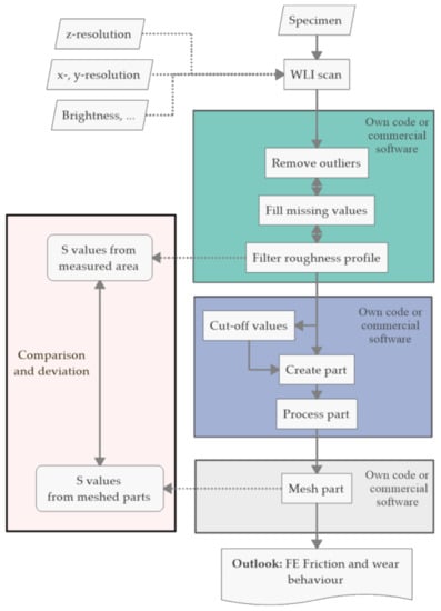
Figure 1.
The method for transferring rough surfaces to FE meshed parts. The validation step of the process comprises the comparison between the surface roughness values (S values) from the measured surface and the S values computed from the meshed part’s surface.
The method started with the scan of a real surface of a physical specimen. A white-light-interferometer-type FRT CWL from FRT GmbH was used for the investigation but could be replaced by other instruments for surface scanning, such as confocal or atomic force microscopes. The result was a neutral text file which contained the surface coordinates for each scanned point. The data set contained non-measured values and outliers, which were removed before filtering the profiles according to DIN ISO 16610 []. The filtered surface was the base for the S value computation according to DIN EN ISO 25178 []. The resulting S values have been later used for the comparison with the S values, which were computed based on the surface mesh nodes. The S values, more precisely the arithmetical mean height (Sa), the maximum height (Sz), the maximum peak height (Sp), and the core height (Sk), were selected for the comparison because they are used in many technical processes (e.g., quality assurance). Similar S values (Spk, Spd, …) are applicable if a considered technical application relies on them. Further descriptions of the surfaces with, e.g., power spectrums are possible, but require a more advanced comparison methods. For this reason, this investigation focuses on the broadly used S values.
The filtered surface data was still available as a neutral text file. The next step was the generation of an iges CAD part. To do so, a MATLAB (The Mathworks, Inc., Portola Valley, CA, USA) routine was used to create a 3D cuboid solid body with length and width according to the real surface data. The routine then generated splines for each vertical and horizontal line of data points and combined them to an analytical surface. This analytical surface (its height data) is mapped by the routine to one side of the cuboid. The result is an iges part, which was imported to CAD software Creo Parametric 5 (PTC). The use of CAD software allows one to easily process the part. Processing steps in the CAD software were, e.g., cutting out specific areas of the surface or removing faces. Since the spline generation creates a 3D part, the removing of faces was done to create 2D surfaces for this investigation.
The 2D iges file, which resulted from the process step, was imported into HyperMesh 2020 (Altair HyperWorks™, Troy, MI, USA). All surfaces were meshed by the auto mesh functionality in the three categories coarse (10 µm), medium (7.5 µm), and fine (5 µm) and by triangle and quadrilateral first-order elements. No other settings (e.g., biasing, node shifting, or further adjustments) were made.
Since the mesh is a key part in every FE simulation, engineers carefully create and analyze it before the computation of a simulation. Most engineers use triangle (resp. tetrahedral) and quadrilateral (resp. hexahedral) elements and therefore these two types were chosen for the investigation of their influence on the depiction of the real surface roughness. Furthermore, the element size is another key factor for the mesh, which engineers often take for a parameter study and to analyze its influence on the results.
Engineers prefer quadrilateral (resp. hexahedral) elements because they have lower computational costs compared to triangular (resp. tetrahedral) elements. However, triangular elements are necessary to model complex geometries. For contact modelling, the influence of the mesh to the simulation results must be considered. Triangle elements or small mesh sizes can enlarge contact stresses due to increased stiffnesses or decreased local contact area sizes. The regular implemented auto mesh function was used for the mesh creation, since manual mesh creation is too time consuming in product engineering processes. The nodes of the mesh were used for the computation of the S values. The deviations between the S values resulting from the filtered profile and the S values from the meshed surface have been the quality criterions for the method.
Besides the conformity of the mesh, another criterion was the mesh quality. To evaluate the mesh quality, each mesh was assessed by its aspect ratio, and skewness. The aspect ratio describes the relation between the minimum and maximum edge length in an element. If the aspect ratio is 1, all edges have the same length. However, the aspect ratio alone is insufficient to describe the form of an element. Thus, the skewness is necessary. It relates the minimum and maximum angle in an element to the optimal angle for the given form. The quality measures are graphically displayed in Figure 2.
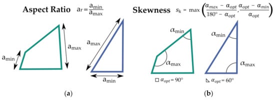
Figure 2.
(a) The computation of the aspect ratio for 2D elements. (b) The computation and determination of the skewness.
2.1. Probes
2.1.1. Probe Preparation
The method is presented by using six specimens with different technical rough surfaces, which were manufactured by different processes and from different materials. The first three surfaces were three sections of one shaft. The sections were turned with different feed rates to get different S values. These specimens are examples for turned surfaces which are commonly used in journal or ball bearings. The shaft’s material was SJ235 steel. Surface four from a graphite-coated plate was used for micro tribological sliding tests (Figure 3). This specimen origins from an investigation of the graphite friction behavior [] and shows the structure of a coated surface. The brake disc was made from cast iron. The final manufacturing step was a surface turning. The brake pad was made of an unknow material composition and bonded to a metal back plate. Both parts were from an SUV brake system (Figure 4). In this investigation, these two parts represent surfaces of a real technical system.
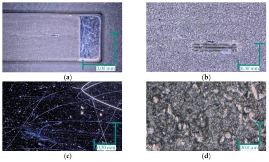
Figure 3.
(a) Iron plate with a microtribometer path. (b) Detailled view of the microtribometer path. (c) Polished iron surface. (d) Graphite surface. (See [] for the results of the investigation of the friction behavior).
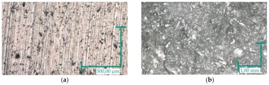
Figure 4.
(a) Turned surface of the brake disc. (b) Surface of the brake pad.
2.1.2. Surface Scanning
All six surfaces were scanned by a commercial white-light interferometer. Three sensor heads were available with a vertical range of 300, 600 and 3000 µm. The three surfaces of the shaft were scanned with the 300 µm sensor head of the white-light interferometer and with a lateral resolution of 2.5 µm. The scanning results are depicted in Figure 5a–c. The surfaces show directional manufacturing marks. The three different Sz values (5.85, 8.99 and 12.15 µm) resulted from different feed rates of turning.
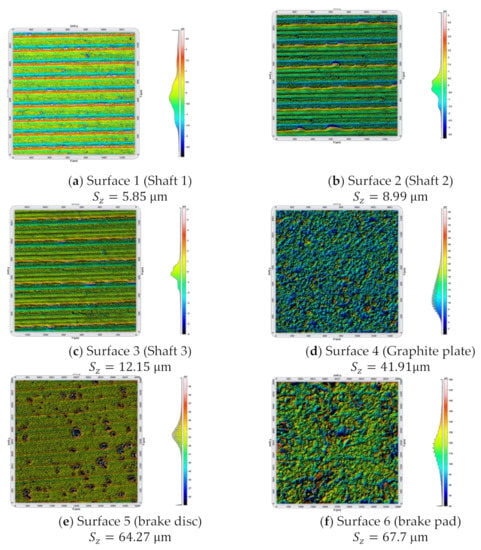
Figure 5.
Surfaces of the six specimens with the height distribution.
The graphite surface was scanned with the 300 µm sensor head and the same settings as the shaft surfaces. The z-range increased to about 40 µm. The multiple hills on the surface originated from the airbrush coating. The substrate plate was made of iron (99.5%) and polished before the coating. The graphite dispersion (L-GP 386 ACHESOR, Henkel) was applied by airbrush in 30 consecutive swipes. The surface showed some hills (referred to as rounded asperities), but most of the coating lied low since the Sa value was 4.06 µm.
A new and unused brake disc was scanned with a lateral resolution of 5 µm. The entire scan area was quadratic with an edge length of 5 mm. The initial surface showed horizontal manufacturing tracks. Because the initial surface is hardly relevant for the function of a brake, the manufacturing was carried out in a time-efficient manner. This means that the turning was performed with a high feed rate, which resulted in breakouts from the surface. These craters were visible in the surface. The brake pad was made of an indefinite mixture of materials. Each material had different transmission, absorption, and reflection attitudes. These materials made the measuring with white-light difficult because the reflection properties differed within one measuring point, whereas all previous specimens had—throughout a scan—a homogenous surface. A successful measuring was possible if the multi-scan option was set. By this option, multiple surface scans were conducted, and the resulting surface was the average value. Figure 5f shows the mountainous surface with some plateaus and deep valleys. The various structures with high plateaus, hills, peaks, and valleys resulted from the mixture of the materials. All surface roughness values are presented in Table 1.

Table 1.
S values computed on base of the measured surface data.
2.1.3. CAD Part Creation
The surfaces, available as digital point clouds, were the base for the creation of the CAD parts. Surfaces 1 to 4 were transferred without modifications by a 2D spline computation to CAD parts with iges file format. This allows one to easily cut the CAD parts into the desired sizes, which was a quadratic area of 1000 µm × 1000 µm. Secondly, the export to the desired geometry file format was easily possible by CAD software.
The first attempts to mesh the unchanged surface of the brake disc showed that the mesh algorithms did not cope with large height differences (cf. Sz values). Therefore, it was advantageous to cut off deep valleys before the spline generation. Figure 6e,f, show the CAD surface after deep valleys were cut off. With Surface 6, a peak cut-off value was set, also before the spline generation. This cut off is feasible, since the computation of the functional R values according to [] includes the same step. This is due to the immediate removal of the highest peaks if contact arises.
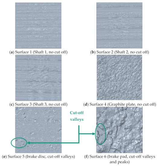
Figure 6.
The real rough surfaces were transferred to CAD parts. The last two surfaces required cutting off some valleys and some peaks before creating the CAD parts.
All resulting CAD parts are displayed in Figure 6. The vertical and horizontal lines rose from the spline generation and served as support lines for the following mesh generation.
2.1.4. Meshing
The meshing was conducted with HyperMesh 2020. Each surface was meshed with three global seed lengths of 10 µm (coarse), 7.5 µm (medium) and 5 µm (fine) with triangle (tri) and quadrilateral (quad) elements. This resulted in six meshes per surface and in total 36 meshes. The auto mesh function was used and no other settings (e.g., biasing, node shifting, or further adjustments) were made.
3. Results
3.1. Graphical Evaluation of Meshes
The meshes of Surface 1 are displayed in Figure 7. The depiction of the manufacturing marks in the mesh increased with a decrease in the element sizes. In the quadrilateral meshes (Figure 7a–c), support lines are visible. These lines were created by the spline generation. The mesh algorithm took the lines as support values for the node and element creation. Since the lines follow the surface topography, these lines did not interfere with the height coordinates itself and therefore did not influence the results. The element orientations at the support lines hamper a clear visibility of the rough surface. However as expected, with decreasing element size the ability to depict the real surface increases, as can be seen in the columns in Figure 7. This means that the finer mesh created a better representation of the real surface. Surface 2 and Surface 3 were similar to the one shown in Figure 7. The elements clearly depict the surface topography which had been exported from CAD software. With triangle meshes, the spline support lines were used for node creation by the mesh algorithm. For this reason, they are clearly visible in the triangle meshes.
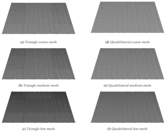
Figure 7.
Triangle and quadrilateral meshs of Specimen 1. In all subfigures, the turning marks are visible as vertical lines. With decreasing seed size, the marks get more clearly visible. (a–c) show a pattern, which results from the mesh algorithm, which takes the edges as support lines.
Figure 8 displays the meshed surface 4 (graphite plate). The mesh algorithm finely coped with the asperities and valleys in both mesh types. A zoom-in in Figure 8d showed that the quadrilateral mesh consists of circular structures. These circular structures consist of a few triangle elements, which increase the depiction precision of the mesh. The quadrilateral mesh coped fine with the asperities and valleys, although the real surface contained medium-high surface gradients. Noticeably, much more elements were required for the triangle fine mesh. The quadrilateral mesh requires about 40,000 elements and the triangle mesh about 80,000 elements.
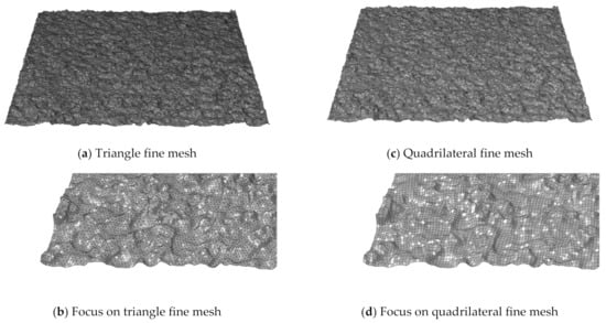
Figure 8.
Triangle and quadrilateral mesh of Surface 4 (graphite plate). The graphite asperities and valleys show, in case of a quadrilateral mesh, a partial circular element layout. The triangle mesh copes fine with the higher gradients.
The meshed surfaces have a good graphical (qualitative) agreement with their real surfaces, since the hills and valleys are clearly depicted by the elements. The graphical differences between the triangle and quadrilateral meshes occur due to the different form of the elements. The quantitative comparison follows in Section 3.2. In contrast to Surfaces 1–5, Surface 6 contained high gradients even with a valley cut-off value. Figure 9 displays the triangle and quadrilateral fine meshes of the brake pad surface. Both meshes contained strongly distorted elements in the top left area of the surface. The zoom-in view in Figure 9b,d reveals many badly shaped elements, which were clearly not suitable for any FE simulations. Further attempts with different mesh algorithms in different software failed too. At steep slopes, the algorithms created nodes at the bottom, on the steep slopes themselves, and on the top. This resulted on the one side in highly deformed elements. On the other side, these elements had acute angles to neighboring elements. Attempts to mesh the surfaces in three dimensions resulted in areas with elements of negative volume.
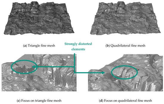
Figure 9.
Surface 6 (brake pad) triangle and quadrilateral fine meshes. Both meshes show in the top left corner many deformed elements. In the zoom-in pictures in (b,d), the mesh has strong distortions in both mesh types, which would not allow a proper FE simulation.
3.2. Comparison of the S Values
For the comparison, the S values were computed based on the filtered surfaces and based on each meshed surface. The deviation describes the percentage difference of a corresponding value between the real and a meshed surface. A negative value means that the value from the mesh is lower than the corresponding measured value. Table 2 gives the values for the minimum and maximum deviation for each surface over all meshes. The results for each mesh are given in Section 3.2.1, Section 3.2.2 and Section 3.2.3.
Table 2.
Minimum and maximum deviation over all six meshes of each surface in comparison to the originally measured values.
3.2.1. Surfaces 1–3 (Turned Shaft)
The deviations of the Sa values of Surfaces 1–3 was continuously increasing from the maximum value −3.5% to a minimum value of −13.6%. So, the meshed surface 3 coped worse with its real surface than Surface 1 with its corresponding real surface. If the focus lies on the individual mesh, all meshed surfaces of Surface 1 coped fine with the real surface according to the Sa value, since the difference of minimum and maximum is just 1.1%. The Sz and Sp values have larger deviations, but the coarse triangle and quadrilateral meshes were positive outliers, as Figure 10a displays. The Sk values followed the negative tendency of the Sa values. The Sp deviation increased with finer meshes. No relation between the mesh type or the mesh size with the deviation was found in the results of Surface 1. Although, the Sa and Sk results of Surface 2 show (cf. Figure 10b) that with decreasing mesh size the deviation decreased, too. By contrast, the Sz and Sp values strongly differed, even with increasing the mesh size. The last surface of the set showed the largest deviations in terms of Sa and Sk values. Most of the Sz and Sp deviations were below 10%. All turned surfaces had in common that the Sa and Sk values decreased, whereas the Sz and Sp values increased, with a finer mesh size. No clear relation between the mesh type or size was noticeable.
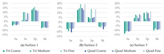
Figure 10.
S value deviations of Surfaces 1–3 (Shaft 1–3).
3.2.2. Surface 4 (Graphite-Coated Plate)
Figure 11 depicts the results for the graphite-coated plate. The Sa deviations are in a similar range as the values for the shafts’ surfaces. The Sa and Sk values are between −4% and −12%. However, the deviations for Sz and Sp are negative, too. The Sp values show that with decreasing the mesh size a better representation of the real surface can be achieved. So, an effect of the mesh size is visible since the deviations reduce with decreasing mesh size for each S value.
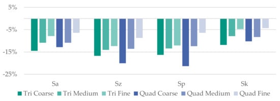
Figure 11.
S value deviation of Surface 4 (graphite-coated plate).
3.2.3. Surfaces 5 (Brake Disc) and 6 (Brake Pad)
The first attempts to mesh Surface 5 failed because the topography gradients hampered a mesh generation. The problems were deep valleys of the outbreaks and steep slopes. Consequently, the valleys were cut off and by these steep slopes slightly reduced. For the use of the surfaces in tribological simulations, the valleys were assumed not to be as tribologically active as asperities because the asperities touch first. In case of particle or fluid simulations, this assumption has to be carefully revised.
The coincidence of the Sa values for the meshed surfaces of the brake disc lied beneath −20%. In contrast, the functional Sk values deviate less than 5%. The Sz and Sp values describe large deviations of about −80%. These result from the cut off before the mesh generation. However, the differences between the deviations are small (cf. Table 2). This means that the surface itself was finely meshed, but its original geometry was changed in comparison to the real surface.
The cut off with Surface 6 (the brake pad) is even clearly visible in Figure 6f. The surface had a graphically bad mesh, which obviously cannot be used for FE simulations. As a result of the adaptions, the deviations themselves lie between −23% and +14% (cf. Figure 12b). Some meshes were able to depict the S values of the real surface, but as the graphical evaluation showed earlier, the graphical quality was in general bad. So, the variation between the meshes is large and the values do not follow any pattern (cf. Figure 12a). The bad graphical mesh and the inconsistency of the S values show that this surface has been difficult to mesh and the present surface cannot be used for an FE simulation.
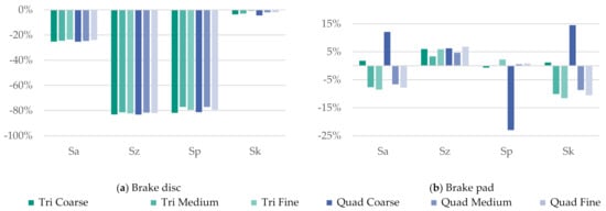
Figure 12.
S value deviation of Surface 5 (brake disc) and Surface 6 (brake pad).
3.3. Mesh Quality
Besides the conformity of the S values, the mesh quality is focused on in this work. The mesh quality has a large impact on the computation time and the precision of the results. Figure 13 plots the aspect ratios of 500 randomly chosen elements from each mesh of the meshed surface 1 and surface 6 over the element skewness. An aspect ratio of 1 and a skewness of 0 describe a perfect element. So, the more points that are in the lower left corner, the better the mesh.
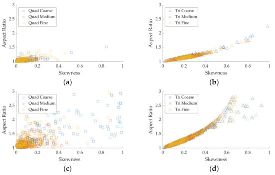
Figure 13.
The vertical axis shows the aspect ratio of 500 randomly chosen elements. The reduction was done because displaying all elements hampered a visibility of the graph. The horizontal axis shows the skewness of the corresponding element. (a,b): Element quality measures for Surface 1 (Shaft 1). (c,d): Element quality measures for Surface 6 (brake pad).
The two top views in Figure 13 show the results for Surface 1. Most of the quadrilateral mesh elements were placed in the lower left corner. This confirmed that the mesh had a good quality in terms of aspect ratio and skewness. Further, with triangle elements (Figure 13b) a dependence of the aspect ratio, the skewness, and the mesh size is visible. The line-shaped distribution illustrated that the aspect ratio and the skewness corresponded for triangle elements. However, all points in both diagrams were below an aspect ratio of 3 and below a skewness of 0.5. Therefore, the graphs verified a good mesh quality to all meshes of Surface 1.
In contrast to the mesh quality of Surface 1, the mesh of Surface 6 shows bad measures in Figure 13. Many elements lie scattered in the entire range of both plots. This phenomenon shows that the mesh quality of Specimen 6 was bad. High aspect ratios and high levels of skewness depict the strongly deformed elements, which were observed in Figure 9. During a simulation, these elements might probably strongly deform, and the computation will abort at early stages.
Table 3 lists in the first column the average aspect ratio () for the six meshes of each surface. The second column comprises the standard deviation of the aspect ratio () distribution. Hereby, low values indicated a low spreading of the aspect ratios for all elements. In case of a high standard deviation, the element aspect ratios revealed larger differences. The next two columns unveil the percentage of elements with aspect ratios larger than 3 and 10. Often, regular FE software uses these two values as limits. The average skewness () and the skewness standard deviation () have a similar meaning to the values in the first two columns.
Table 3.
Mean aspect ratio, standard deviation of aspect ratio, percentage of elements with aspect ratio larger 3, percentage of elements with aspect ratio larger 10, mean skewness and standard deviation of skewness.
Surface 1 and surface 2 had similar results for aspect ratio and skewness distribution. Low deviations and no elements with aspect ratios above 3% revealed a good mesh. Surface 3 meshes had a larger deviation and even 0.02% strongly distorted elements. However, the S value deviation indicated the best coincidence in comparison between Surfaces 1–3 (cf. Table 2).
Surface 6 (brake pad) had large deviations and bad mesh quality measures. Moreover, in each column of Table 2, it had the worst values and even 0.2% strongly deformed elements. This mesh would be not suitable for FE simulations.
4. Discussion and Conclusions
The digitalization of Surfaces 1–3 causes an increase in the Sz values. This shows that the minimum and maximum surface values move apart during spline generation and meshing. However, this shrinkage has not affected the Sa values in the same direction, which indicates that the average profile height has slightly reduced during the spline and mesh generation. The directional manufacturing marks, which are visible in Figure 5 and Figure 6, have the highest surface coordinates and therefore determine the Sz and Sp values. The remaining area between the marks determine the Sa and Sk value. So, for pointy topography (with steep peaks and valleys), the digitalization tends to increase the Sz and Sp values. The average points are moved together since the Sa and Sk value are reduced.
Furthermore, a dependence between the Sa and Sk values ca be observed, because in Surfaces 1–3 the corresponding deviations are negative. This behavior is the consequence of the computation of both values being the average surface height values used. The Sa values are computed by the average mean height and the Sk value also focuses on the mean profile area as it is described in []. Thus, a shift or slight change of the mean profile moves both values in the same direction. The same principle is valid for the Sz and Sp values, which correspond to the extreme values of surface. The growth in the Sp values accompanies in all three surfaces a growth in the Sz value.
A close look to the first three rows in Table 2 reveals that most of the deviations are below 10%. However, a clear dependence of the deviation upon a roughness value has not been visible. Neither the Sa nor the Sz value deviation illustrates a tendency in the absolute S values (see Table 1). Even the high Sz value of Specimen 3 has not resulted in a high deviation since the average deviation of all mesh models is just 5.9%.
Surface 4, the graphite-coated plate, has the same decreasing behavior for the Sa and Sk values. In each mesh, the Sa and Sk values underestimate the measured value. The conclusion is that the wavy topography (cf. pointy topography of Surface 1–3 in this section) of the graphite coating is flattened by the spline and mesh generation. In contrast to Surfaces 1–3, the peaks of Surface 4 are flat, which results in reduced Sz and Sp values. The two hypotheses that the Sa values coped with the Sk and the Sp with the Sz value has been confirmed by this specimen’s surface. In the deviations of the graphite-coated plate, a dependence between the mesh size and deviations is observed. With both mesh types, the deviation shrinks with decreasing mesh sizes. Surface 4 is the only surface showing this behavior.
Surface 5, the brake disc, had drops in the Sp and Sz values in comparison to the other surfaces. These drops resulted from the cut off. The drop of the Sz and Sp values affected the Sa values, too. The Sk values followed the Sa values again. However, the surface was flattened by the cut-off values, but the low variations in the mesh deviations and the mesh quality confirm the usability of the meshes for FE simulations.
The last surface, the brake pad, shows for isolated meshes low deviations. However, the comparison of the meshes reveals large fluctuations, which would give a good measure if only one mesh is considered. Furthermore, the graphical check of the mesh and the mesh quality measured illustrate largely deformed elements, which are not suitable for an FE simulation.
In FE simulations, small mesh sizes allow for a more precise depiction of local stress states. Thus, engineers use small mesh sizes for relevant areas. Relevant areas are not modelled with larger mesh sizes to reduce the number of elements and by this the necessary computation time. Surfaces, which are meshed with linear triangle (or tetrahedral) elements, usually result in higher contact pressures because the linear ansatz functions tend to increase the stiffness. Similar behavior can be observed with the mesh size. Smaller mesh sizes generally result in a more precise contact depiction but increase the maximum contact pressures due to smaller local contact areas. However, the results for the deviations show that decreasing the mesh size does not generally correlate with a more precise depiction of the surface. Moreover, the use of triangle or quadrilateral elements does not influence the depiction ability of the entire mesh. So, finer meshes do not result in a better coincidence of the S values. However, a firm agreement of the mesh and the real surface shall be worked towards.
The last evaluation, the mesh quality measures, illustrates that those regular commercial algorithms do not cope well with real surfaces with high surface gradients, which the brake pad comprises. In contrast, Surfaces 1–3 are finely meshed in all six mesh cases. The small outlier values of Surface 3 do not represent a common case for this element size, as shown by the remaining meshes. Surface 4 is finely meshed with either triangle or quadrilateral elements. Surface 5 is finely meshed too and can be used for further simulations. Only the last surface shows strong mesh outliers, which cannot be easily solved. The spikes and deep cliffs show that strong surface gradients cannot be well meshed. The regular commercial algorithms do not cope with the steep cliffs.
5. Conclusions
This investigation presents a method for the transfer of real rough surfaces to FE simulations. Furthermore, the degree of agreement between the measured surface and meshed surface is assessed by the deviation of the S values. At last, mesh quality measures are used to evaluate the meshes. The degree of agreement is hereby presented for regular roughness values according to DIN EN ISO 25178 []. Similar values such as Spk or Spd are analogously usable for the assessment of surfaces.
In case of transferring real into virtual surfaces, the surfaces should be examined graphically to identify steep slopes or valleys that result in difficulties during meshing. Furthermore, the simulation method must be considered at the beginning. If it is, for example, a computational fluid dynamic (CFD) or an FE analysis, this can already be considered during processing. CFD simulations can require valleys for analyzing contact flows, whereas the valleys can be some FE simulations ca. Considering different mesh sizes, the comparison of the S values shows the ability of the meshing algorithm to be able to mesh the surface. Thus, the comparison of the real measured surfaces with the meshed surfaces is an important step for the evaluation of the transfer. The choice of the S values is dependent on the target application. A difference in meshing with triangular and quadrilateral elements was not found. Possible recommendations of an FE solver can be considered here.
The mesh quality (aspect ratio and skewness) is computed and turned out to be a valuable measurand for an FE mesh. The aspect ratio and skewness are scores for the depiction of the mesh quality. Large values of the aspect ratio show a distorted mesh. For the comparison of similar meshes, the measure is an indispensable score in FE computations. The scatter plot (see Figure 13) graphically compares different meshes using the aspect ratio and the skewness. Strongly distorted elements are easily noticeable by outliers in the graph.
This method enables researchers and engineers to transfer rough surfaces to CAD parts and mesh geometries. The individual steps of the procedure are designed to be replaced by any desired method. For example, the hereby used white-light interferometer can be easily replaced by a confocal microscope or atomic force microscope. The use of regular CAD software allows one to use the surface as 3D parts for any other relevant application, e.g., rendering.
The mesh is conducted by commercial algorithms for 2D on the base of a spline-generated surface. A direct mesh generation on the base of the surface point data is possible, but this requires time-consuming self-written code. Because the concentration lies on engineering processes, the focus was put on regular commercially available solutions. Furthermore, a 3D mesh can be achieved with the created CAD solid bodies.
Tribological simulations are conducted with a vast variety of surfaces, e.g., casted, transformed, turned, milled, coated, oxidized, or varnished. Further research could compare different surfaces which result from different production technologies. In particular, additive manufactured parts are as rare as tribological active surfaces but will gain importance. Therefore, the next step could be the analysis of additive manufactured parts with FE simulations or the use of different comparison methods, such as power spectrums.
Further topics about this investigation will concern the computation of meshes by directly using the surface point data. This requires the development of new mesh algorithms, which can be used for multiple input formats. Extensions for already available commercial algorithms can improve their ability to generate fine meshes of real unstructured surfaces.
Author Contributions
Conceptualization, A.J. and S.R.; methodology, A.J., S.R. and A.A.; software, C.W.; validation, N.S.A.; writing—original draft preparation, A.J.; writing—review and editing, A.J., S.R., N.S.A., C.W. and A.A.; funding acquisition, A.A. All authors have read and agreed to the published version of the manuscript.
Funding
The authors thank the Deutsche Forschungsgemeinschaft (DFG) for the funding of the project “Mechanism of Graphite Lubrication in Rolling Contact” (“Mechanismen der Graphitschmierung in Wälzkontakten”), grant numbers AL533/37-1. The project is part of the priority program “SPP 2074: Fluidless Lubricationsystems with high mechanical Load” (“SPP 2074: Fluidfreie Schmiersysteme mit hoher mechanischer Belastung”).
Acknowledgments
The authors thank Martin Dienwiebel (Karlsruhe Institute of Technology (KIT), IAM–CMS Institute for Applied Materials–Computational Materials Science, MicroTribology Center µTC) for supplying the graphite plate as specimen for this investigation.
Conflicts of Interest
The authors declare no conflict of interest.
References
- Holmberg, K.; Erdemir, A. Influence of tribology on global energy consumption, costs and emissions. Friction 2017, 5, 263–284. [Google Scholar] [CrossRef]
- German Institute for Standardization. DIN EN ISO 4287 Geometrische Produktspezifikationen (GPS)—Oberflächenbeschaffenheit: Tastschnittverfahren—Benennung, Definitionen und Kenngrößen der Oberflächenbeschaffenheit (ISO 4287:1997 + Cor 1:1998 + Cor 2:2005 + Amd 1.2009); Deutsch Fassung EN ISO 4287:1998 + AC:2008 + A1:2009; Beuth Verlag GmbH: Berlin, Germany, 2010. [Google Scholar]
- German Institute for Standardization. DIN EN ISO 4288 Oberflächenbeschaffenheit: Regeln und Verfahren für die Beurteilung der Oberflächenbeschaffenheit; Beuth Verlag GmbH: Berlin, Germany, 1998. [Google Scholar]
- German Institute for Standardization. DIN EN ISO 13565-1 Oberflächenbeschaffenheit: Tastschnittverfahren: Oberflächen mit Plateauartigen Funktionsrelevanten Eigenschaften Teil 1: Filterung und Allgemeine Meßbedingungen (ISO 13565-1:1996) Deutsche Fassung EN ISO 13565-1:1997; Beuth Verlag GmbH: Berlin, Germany, 1998. [Google Scholar]
- German Institute for Standardization. DIN EN ISO 13565-2 Oberflächenbeschaffenheit: Tastschnittverfahren: Oberflächen mit Plateauartigen Funktionsrelevanten EigenschaftenTeil 2: Beschreibung der Höhe Mittels Linearer Darstellung der Materialanteilkurve (ISO 13565-2:1996) Deutsche Fassung EN ISO 13565-2:1997; Beuth Verlag GmbH: Berlin, Germany, 1998. [Google Scholar]
- Quinten, M. A Practical Guide to Surface Metrology; Springer International Publishing: Cham, Switzerland, 2019. [Google Scholar]
- Jiang, X.; Scott, P.; Whitehouse, D.; Blunt, L. Paradigm shifts in surface metrology. Part I. Historical philosophy. Proc. R. Soc. A 2007, 463, 2049–2070. [Google Scholar] [CrossRef] [Green Version]
- German Institute for Standardization. DIN EN ISO 16610-61 Geometrische Produktspezifikationen (GPS)—Filterung Teil 61: Lineare Flächenfilter: Gauß-Filter (ISO16610-61:2015): Grundlegende und Allgemeine Begriffe und Zugeordnete Benennungen (VIM) Deutsch-Englische Fassung ISO/IEC-Leitfaden 99:2007; Beuth Verlag GmbH: Berlin, Germany, 2016. [Google Scholar]
- German Institute for Standardization. DIN EN ISO 25178-2 Geometrische Produktspezifikation (GPS)—Oberflächenbeschaffenheit: Teil 2: Begriffe und Oberflächen-Kenngrößen (ISO 25178-2:2012); Beuth Verlag GmbH: Berlin, Germany, 2012. [Google Scholar]
- Gao, F.; Leach, R.K.; Petzing, J.; Coupland, J.M. Surface measurement errors using commercial scanning white light interferometers. Meas. Sci. Technol. 2008, 19, 15303. [Google Scholar] [CrossRef] [Green Version]
- Spencer, A.; Dobryden, I.; Almqvist, N.; Almqvist, A.; Larsson, R. The influence of AFM and VSI techniques on the accurate calculation of tribological surface roughness parameters. Tribol. Int. 2013, 57, 242–250. [Google Scholar] [CrossRef]
- Persson, B.N.J. On the Fractal Dimension of Rough Surfaces. Tribol. Lett. 2014, 54, 99–106. [Google Scholar] [CrossRef]
- Hu, Y.Z.; Tonder, K. Simulation of 3-D random rough surface by 2-D digital filter and fourier analysis. Int. J. Mach. Tools Manuf. 1992, 32, 83–90. [Google Scholar] [CrossRef]
- Putignano, C.; Afferrante, L.; Carbone, G.; Demelio, G. A new efficient numerical method for contact mechanics of rough surfaces. Int. J. Solids Struct. 2012, 49, 338–343. [Google Scholar] [CrossRef] [Green Version]
- Pérez-Ràfols, F.; Almqvist, A. Generating randomly rough surfaces with given height probability distribution and power spectrum. Tribol. Int. 2019, 131, 591–604. [Google Scholar] [CrossRef]
- Graf, M.; Ostermeyer, G.-P. Instabilities in the sliding of continua with surface inertias: An initiation mechanism for brake noise. J. Sound Vib. 2011, 330, 5269–5279. [Google Scholar] [CrossRef]
- Hetzler, H.; Willner, K. On the influence of contact tribology on brake squeal. Tribol. Int. 2012, 46, 237–246. [Google Scholar] [CrossRef]
- Abu Bakar, A.R.; Ouyang, H.; James, S.; Li, L. Finite element analysis of wear and its effect on squeal generation. Proc. Inst. Mech. Eng. Part D J. Automob. Eng. 2008, 222, 1153–1165. [Google Scholar] [CrossRef]
- Wenk, J.F.; Stephens, L.S.; Lattime, S.B.; Weatherly, D. A multi-scale finite element contact model using measured surface roughness for a radial lip seal. Tribol. Int. 2016, 97, 288–301. [Google Scholar] [CrossRef]
- Fischer, F.; Murrenhoff, H.; Schmitz, K. Influence of normal force in metallic sealing. Eng. Rep. 2021, e12399. [Google Scholar] [CrossRef]
- Zhang, F.; Liu, J.; Ding, X.; Wang, R. Experimental and finite element analyses of contact behaviors between non-transparent rough surfaces. J. Mech. Phys. Solids 2019, 126, 87–100. [Google Scholar] [CrossRef]
- Albers, A.; Reichert, S.; Joerger, A. Investigation of roughness parameters of real rough surfaces due to sliding wear under mixed-lubricated conditions with the finite-element-method. In Proceedings of the World Tribology Congress 2017, Beijing, China, 17–22 September 2017. [Google Scholar]
- Albers, A.; Behrendt, M.; Klingler, S.; Reiß, N.; Bursac, N. Agile product engineering through continuous validation in PGE—Product Generation Engineering. Des. Sci. 2017, 3, e5. [Google Scholar] [CrossRef] [Green Version]
- Morstein, C.E.; Dienwiebel, M. Graphite Lubrication Mechanisms under High Mechanical Load. Wear 2021, 477, 203794. [Google Scholar] [CrossRef]
Publisher’s Note: MDPI stays neutral with regard to jurisdictional claims in published maps and institutional affiliations. |
© 2021 by the authors. Licensee MDPI, Basel, Switzerland. This article is an open access article distributed under the terms and conditions of the Creative Commons Attribution (CC BY) license (https://creativecommons.org/licenses/by/4.0/).