Article

Impact of Constant Versus Fluctuating Temperatures on the Development and Life History Parameters of Aldrichina grahami (Diptera: Calliphoridae)

1
Department of Forensic Science, School of Basic Medical Sciences, Central South University, Changsha 410013, China
2
Department of Forensic Science, School of Basic Medical Sciences, Xinjiang Medical University, Urumqi 830011, China
*
Author to whom correspondence should be addressed.
These two authors contributed equally to this work.
Insects 2019, 10(7), 184; https://doi.org/10.3390/insects10070184
Submission received: 7 May 2019 / Revised: 14 June 2019 / Accepted: 18 June 2019 / Published: 26 June 2019

Abstract

:
Necrophagous fly species are commonly used as forensic tools to estimate the minimum postmortem interval (PMImin). Many researchers raised necrophagous flies under constant temperature regimes to collect their developmental data. However, in most forensic cases, the ambient temperature fluctuates. In order to investigate a forensically important fly developmental mode (the Isomegalen diagram, Isomorphen diagram and Thermal summation models) and make comparisons of the developmental rate between constant temperatures and fluctuating temperatures, we used Aldrichina grahami (Diptera: Calliphoridae) to investigate the life history parameters at eight constant temperatures ranging from 8 to 36 °C. We also compared developmental rate of A. grahami in three groups of constant versus fluctuating temperatures: 8 °C vs. 6–12 °C, 12 °C vs. 10–16 °C, and 16 °C vs. 14–20 °C. Our data showed that A. grahami is cold tolerant with a mean (±SE) development threshold temperature (D0) of 3.41 ± 0.48 °C and a thermal summation constant (K) of 8125.2 ± 288.4-degree hours. The three groups subjected to fluctuating temperatures took longer to develop compared to those developing in constant temperatures when simulated in a model. These results not only provide detailed developmental data for the use of A. grahami in the estimation of the PMI, but also indicate that ambient temperature fluctuation must be taken into consideration for the use of all necrophagous fly species.

1. Introduction

Forensic entomology is the science of collecting and analyzing insect evidence to aid in forensic investigations [1]. Forensic entomologists can use developmental data of sarcophagus insects to determine the minimum post mortem interval (PMImin) or the time since insect colonization of human remains. Forensic investigators link the information of a crime scene or discovery location to the duration of the forensically important insects found on, in or around corpses [2,3]. Blow flies (Diptera: Calliphoridae) are one of the most important families in forensic entomology, and have a cosmopolitan distribution. With a remarkable flying capability and a striking sense of smell, they can locate and reach a corpse in a very short time after death occurs [4,5]. Blow flies are often the first insects colonizing a carcass, making them the most frequently and effectively available insects for PMImin estimation [1,3].
Aldrichina grahami (Aldrich 1930, Diptera: Calliphoridae) is a forensically important species that is mainly distributed in Asia, but it has also been reported to appear in Russia, Mexico and the United States of America [6,7,8,9]. Adults of A. grahami rarely aggregate indoors, and commonly colonize garbage, feces and carcasses [9]. When the ambient temperatures are low (usually from late autumn to the following spring), A. grahami is one of the first species to colonize a corpse, which suggests that this species is relatively cold tolerant [9,10]. Calculation of the PMImin requires the gathering of exact developmental data [3,11]. Hence, we used A. grahami to study the developmental models at both constant temperatures and fluctuating temperatures.
Accurate developmental data of sarcophagus flies are vital for estimation of PMImin. Most experiments on the developmental patterns of forensically important insects under constant temperatures aim to collect data on changes in the length of larval body, developmental stage, and thermal summation [12,13,14,15,16,17,18]. Only a few studies refer to fluctuating temperatures [15,19,20,21,22]. However, in most medicolegal investigations, the ambient temperatures of the scene are variable. As such, we raised sarcophagus flies in the laboratory by imitating the fluctuating temperatures of a scene, using temperature models of climatic conditions naturally occurring in Hunan province (28°12′ N, 112°58′ E), south-central China, in the most active seasons for A. grahami.
In this study, the adults of A. grahami were trapped in the wild to establish a laboratory colony. Collecting developmental data at eight constant temperatures of 8 °C, 12 °C, 16 °C, 20 °C, 24 °C, 28 °C, 32 °C and 36 °C, and three fluctuating temperatures of 6–12 °C, 10–16 °C, 14–20 °C, (average temperatures of three fluctuating temperatures groups were 8 °C, 12 °C, 16 °C). The body length and weight of the larvae varied with accumulated temperature, and developmental durations were used to establish relevant developmental models (the Isomegalen diagram, Isomorphen diagram and Thermal summation models). In addition, we compared the development of A.grahami between fluctuating temperatures and constant temperatures. All these results of A. grahami determined the post-colonization interval and play an important role in the estimation of the PMImin.

2. Materials and Methods

2.1. Establishment of Laboratory Colony

During the season of A. grahami exuberant reproduction in March 2016, in Changsha, China (28°12′ N, 112°58′ E), A. grahami adults were collected from a deserted yard near a reservoir, which was used to discard devalued fish by fishermen. Fifty adult flies were obtained. The fly species identification was performed using the adult identification key according to Fan [23]. The rearing was conducted in an insect laboratory; the temperature of the laboratory was approximately 24 °C, with 70% relative humidity and natural light. Moreover, other insects were prevented from entering this room. Adults were reared in an insect cage (35 by 35 by 35 cm) with the six sides covered by a nylon net using a zipper to conduct switches. A nest feeder and two culture dishes were placed in the cage. The nest feeder was loaded with fresh water ad libitum, and the water channel was covered by a plastic net to serve as a stand when the adult flies drinking. A mixture of sugar and milk powder (1:1) contained in a dish (12 cm in diameter) was used as the food, and 15 g fresh pig lung in another dish was used to induce oviposition. The eggs were reared in a flat-bottomed bowl (18 cm in diameter, 5 cm in height), in a box (25 by 25 by 12 cm) filled with 2–3 cm height of sifted sand to cover the bottom of the box, and placed the box in another insect cage (we called the combination of dish, bowl, box, and cage the biomimetic appliance for rearing larvae). As such, a sufficient amount of fresh pig lung was supplemented at every inspection every day until pupation. To obtain a pure-bred colony for the subsequent study, the flies were cultured for five generations.

2.2. Experiment Condition

We designed the fluctuating temperature models on the basis of the weather conditions in southeast China (http://www.tianqihoubao.com/lishi/changsha.html). For instance, temperatures of 14–20 °C (Fluctuating 16 °C = F16 °C, Constant 16 °C = T16 °C) were used, with the average temperature being 16 °C to imitate weather in April. Temperatures were designed as follows:
-
00:00–06:00 14 °C,
-
06:00–14:00 temperature increasing arithmetically from 14 to 20 °C,
-
14:00–22:00 temperature decreasing arithmetically from 20 to 14 °C,
-
22:00–00:00 14 °C.
The second condition temperatures were from 10 to 16 °C (Fluctuating 12 °C = F12 °C, Constant 12 °C = T12 °C), with average temperatures of 12 °C used to imitate weather in March and November. The third condition temperatures were from 6 to 12 °C (Fluctuating 8 °C = F8 °C, Constant 8 °C = T8 °C), with the average temperatures of 8 °C used to imitate weather in December and February. Detailed information of the three fluctuating temperature conditions is shown in Figure 1. Fluctuating temperature models were designed according to two points: 1, climatic conditions naturally occurring in the Hunan province of China; 2, we simplified the model and increased the convenience of conducting the relevant calculations.
To ensure a sufficient number of eggs, over 1000 adult flies were raised in two big insect cages (100 cm by 100 cm by 100 cm) in the insect room, in the stable oviposition period. No pig lung was provided for one day or more to make an artificial peak oviposition period. A dish containing 20 g of fresh pig lung was placed in the insect cage to induce oviposition, we collected the eggs oviposited after 2 h [24], and recorded the time of oviposition. Egg masses were made containing about 2800 eggs (regarded as a replication), then the eggs were equally divided into two portions, with one portion for constant temperatures and another portion for fluctuating temperatures. To avoid the larvae overcrowding, which would increase the temperature and stimulate the growth of larvae [1], a larger flat-bottomed bowl (22 cm in diameter, 5 cm in height) was used (we would have added another bowl if larvae were overcrowding).
Each portion and 20 g of pig lung were transferred into the biomimetic appliance for rearing larvae, and the biomimetic appliance was placed in a climatic chamber LRH-250-GSI (Taihong Co., Ltd., Shaoguan, China) at constant temperatures of 16 °C. The other portions were placed in the other climatic chamber at fluctuating temperatures of 14–20 °C (each incubators of fluctuating temperatures vs constant temperatures provided same quantity of heat in every 24 h). All climatic chambers had a 75 ± 5% humidity and a photoperiod of L12:D12. Specifically, the temperature was controlled by an electronic system to ensure that the incubators maintained the preset temperatures. In addition, the temperature and humidity of the chambers was monitored by automatic thermohygrograph (FLIR SSN-22 USA). The above experiment was repeated five times in different incubators (each replication put in a separate incubator). The remainder of the two groups of constant temperatures and fluctuating temperatures (12 °C vs. 10–16 °C, 8 °C vs. 6–12 °C) were conducted with the same processes as 16 °C vs. 14–20 °C. In addition, the group of 8 °C vs. 6–12 °C was sampled only once a day. The remaining constant temperatures (20 °C, 24 °C, 28 °C, 32 °C, 36 °C) also followed the procedures as above, with egg masses containing about 1400 eggs as a replication. For each temperature, the experiment was repeated five times.

2.3. Collection of Developmental Data

After oviposition, the eggs were checked hourly and the time of hatching was recorded. In addition, a small piece of fresh pig lung was provided uniformly in the culture bowl to avoid sharp accumulation of larvae-generated heat [25]. A sufficient amount of fresh pig lung was supplemented every eight hours (more frequently in high temperatures) until pupation. The supplement had to meet the requirements of the larvae for development.
The onset of the 1st instar (equivalently, the endpoint of the egg stage) was designated when 50% of the larvae hatched [25]. Ten of the larvae were sampled randomly every 12 h after hatching (more frequently in high temperatures) and immediately placed in >80 °C hot water for 30 s, then preserved in 75% ethanol with the volume doubling that of the larvae at 6 °C for no more than two weeks [11,26,27]. The length of each individual was measured using a digital caliper (Meinaite, Shanghai, China). The larvae were weighed by analytical balance (FA1204B, Shanghai, China). The weight of the larvae had a large variation even for the same cohort. Hence, we just measured the body weight of ten larvae as a single unit. Using a stereomicroscope (Motic SMZ-168) the larval instar was determined according to the number of slits in the posterior spiracle [28]. Moreover, any individual proceeded to the next stage was considered to be at the endpoint of the current stage (i.e., a 1–2 transitional instar was counted as a first-instar larva) [29]. The onset of the pupal stage was designated as the time when 50% of individuals had pupated. The same method was used to determine the wandering period and eclosion. At pupation, pupae were observed every 12 h.

2.4. Data Analysis

Data analysis was performed by the software OriginPro 9.0. One-way ANOVA tested the effect of temperature treatment on the duration of each life stage. The relationship between the larval body length and time after hatching was analyzed using nonlinear regression. The larval body length was used as the independent variable while time after hatching was the dependent variable [25]. The revised regression model proposed by Ikemoto and Takai was used [30]. A linear analysis was conducted to analyze the relationship between developmental duration and accumulated degree hours (ADH) at each developmental stage and the total developmental stages. The slope and y-intercept of the linear regression equation were used to determine the development threshold temperature D0 and thermal summation constant K, respectively.

3. Results

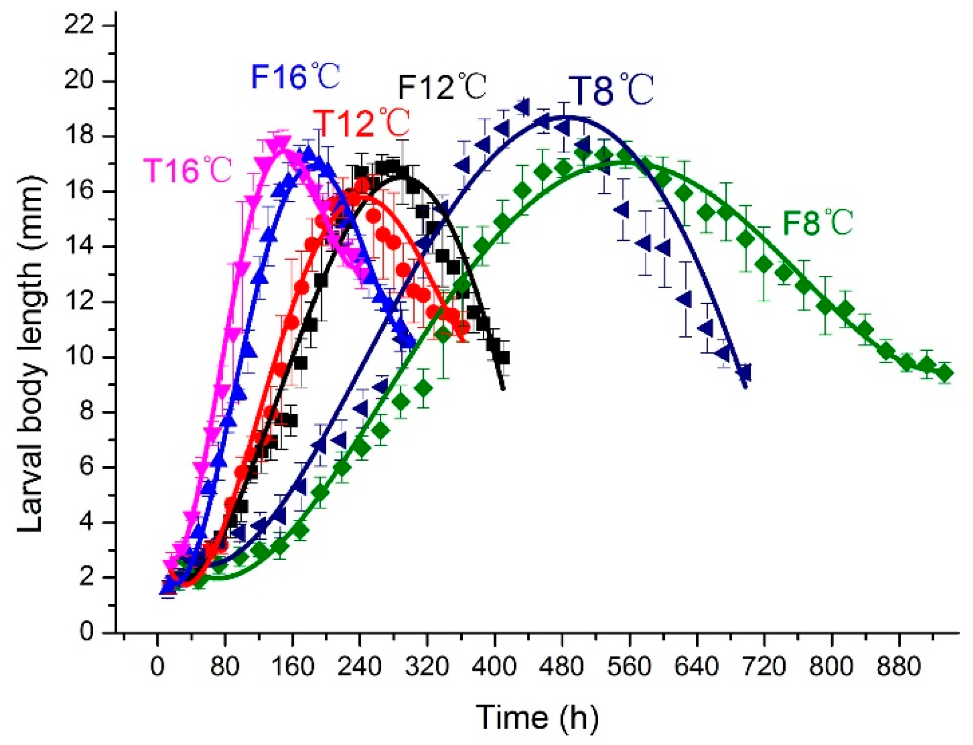
3.1. Constant Temperatures vs. Fluctuating Temperatures

For A. grahami reared in three groups of constant vs. fluctuating temperatures, the durations of every developmental stage decreased with increasing temperature, including the egg, first instar (1st instar), second instar (2nd instar) and third instar (3rd instar) larvae, wandering and pupae (Table 1). In addition, for each fluctuating group, the time of every developmental stage was longer than the matched constant group, and the significant difference became indistinctive with increased temperatures. Each developmental duration from 1st instar larvae to wandering in F8 °C and F12 °C was significantly longer than in T8 °C and T12 °C (Table 1, one-way ANOVA + LSD test at p < 0.05). Notably, the developmental durations of eggs only showed significant differences in 8 °C vs. 6–12 °C. The significant difference was indicated at pupal stage in 16 °C vs. 14–20 °C, and the adults failed to eclose (dead pupa) in the groups of T8 °C, F8 °C and F12 °C (Table 1).
Developmental rate (v) is calculated from developmental duration (h), v = 1/h. Because each fluctuating group had a longer time than the matched constant group in every developmental stage, the developmental rate of fluctuating temperatures was slower than constant temperatures over the whole developmental cycle. We used the time after hatching as the independent variable and larval body length as the dependent variable to obtain the curve fitting equation (Figure 2) and equations (Table 2) of the changes in larval body length of A. grahami. Accordingly, we tested the change in larval body weight with time (Supplementary Materials Figure S1 and Table S2). The larval body weight was connected to larval body length, thus, the rate of weight increase in fluctuating temperatures was slower than in constant temperatures.

3.2. Development in Constant Temperatures

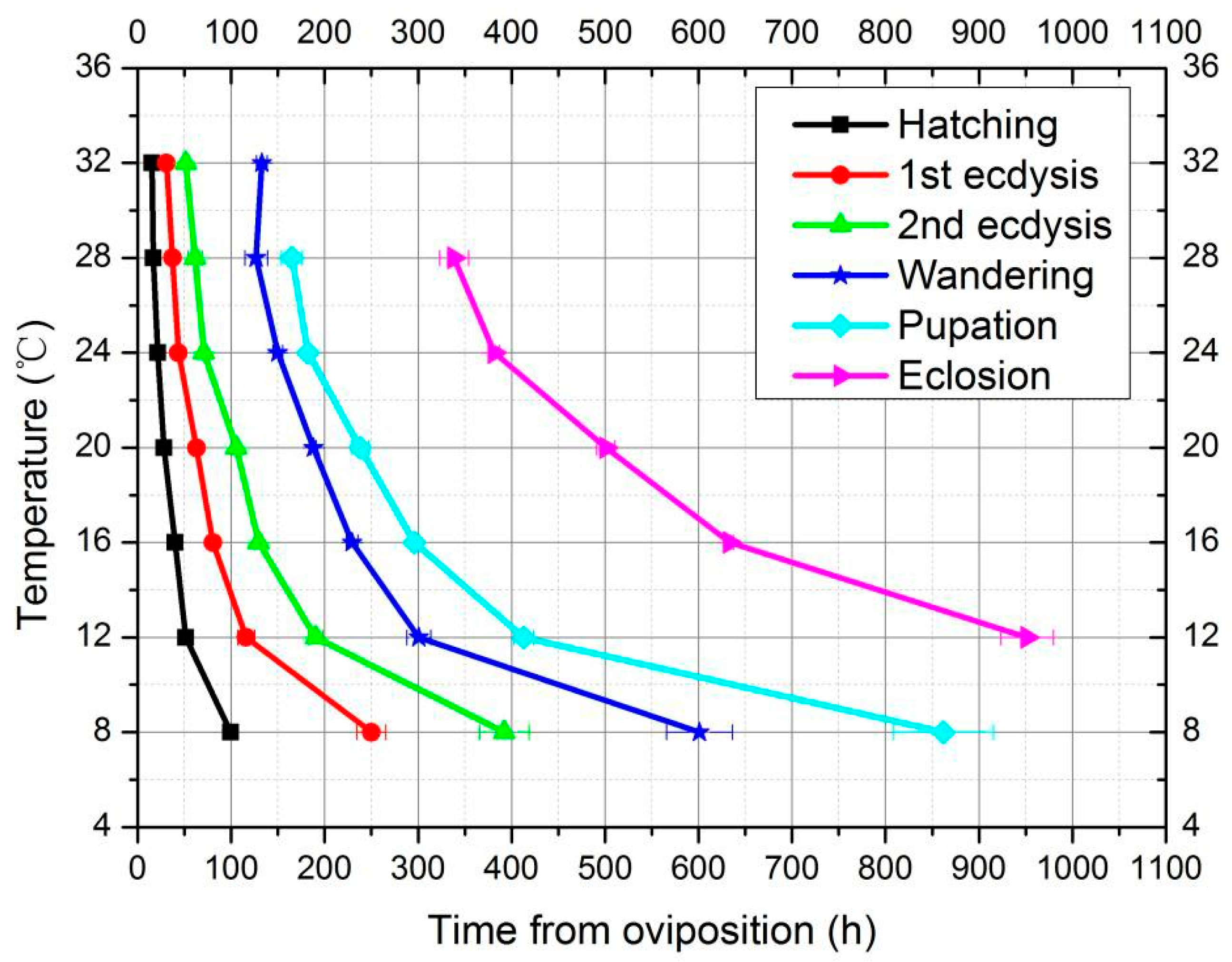
3.2.1. Developmental Duration and Isomorphen Diagram

From constant 12 to 28 °C, the developmental durations of the egg, 1st instar, 2nd instar and 3rd instar larvae, wandering and pupa were decreased. At 36 °C the egg of A. grahami was unable to hatch, and at 8 °C the adults failed to eclose. Besides, two misshapen developmental durations were observed in 3rd instar larvae and were wandering at 32 °C; both developmental durations were unnaturally prolonged (Table 1). The average time of hatching was decreased from 99.3 h at 8 °C to 14.9 h at 32 °C, and the total developmental duration was decreased from 951.6 h at 12 °C to 338.4 h at 28 °C (Table 1).
The isomorphen diagram (Figure 3) was plotted based on the duration of different developmental events (x-axis) at different constant temperatures (y-axis). In the temperature range of 8–32 °C, the duration between each developmental event (hatching, first ecdysis, second ecdysis, pupation and eclosion) gradually decreased as the temperature increased, while only the specific time of the 3rd instar larvae and wandering were prolonged at 32 °C, and the curve displayed an distinct direction compared with the other six temperatures tested. With the temperature increasing, the distance between each curve was gradually shortened.

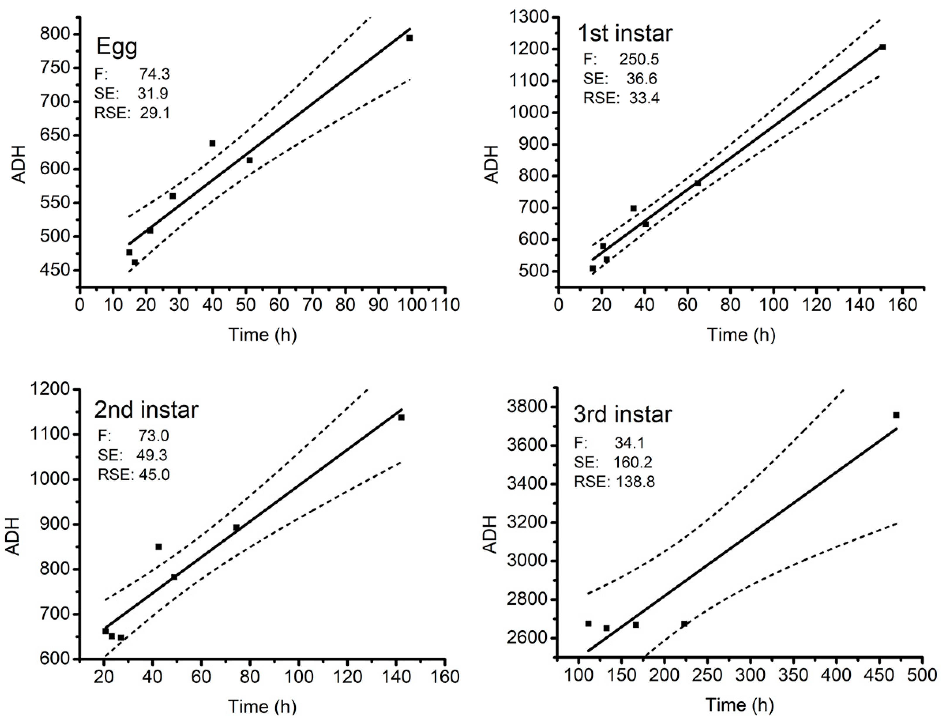
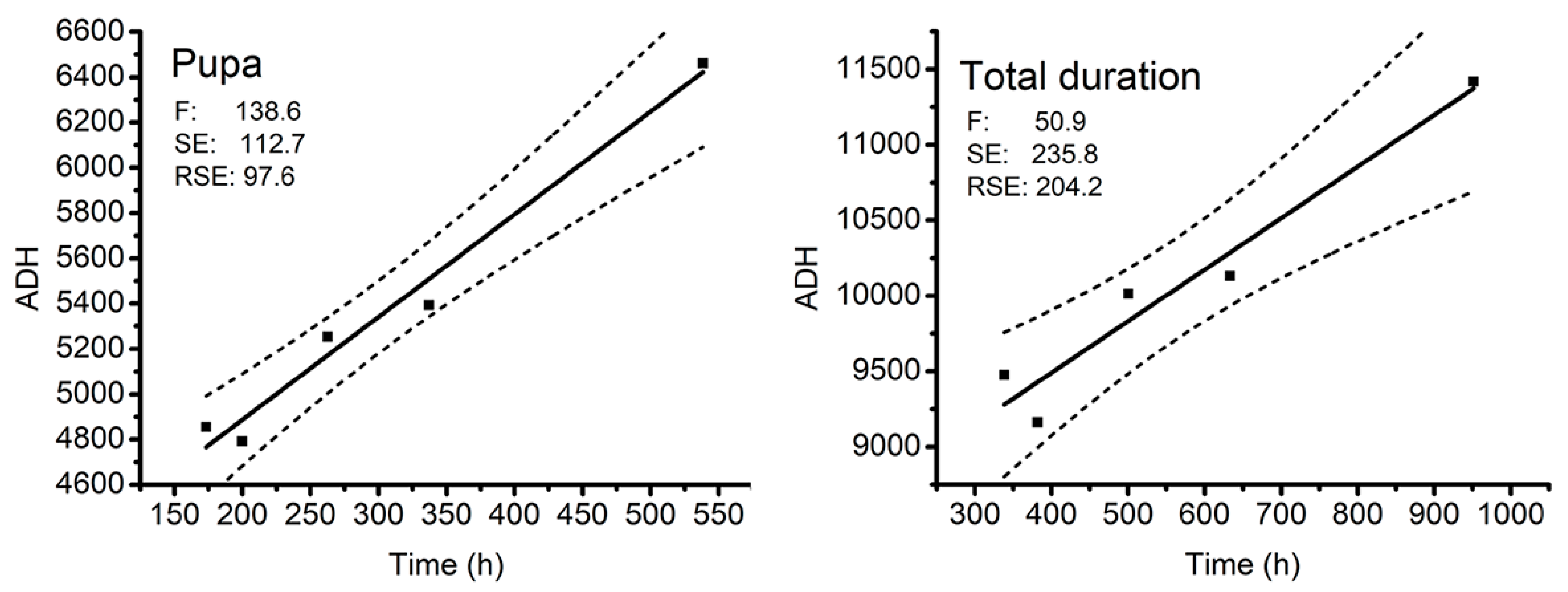
3.2.2. Thermal Summation Model

Six thermal summation models were established by linear regression analyses based on the duration of six developmental events and the entire developmental period as the x-axis and degree hours as the y-axis at each developmental stage (Figure 4). With the exception of the linear regression of 3rd instar larvae with a coefficient of determination (R2) value 0.89, the remaining five thermal summation models all had an R2 value above 0.92, indicating that the data of five models had a relatively good fit to linear models (Table 3). The data of 3rd instar larvae at 32 °C was poorly correlated with linear models. Hence, we rejected these data from the regression analysis. The developmental threshold temperature D0 and thermal summation constant K of A. grahami during the total developmental process calculated by the thermal summation model were 3.41 ± 0.48 °C and 8125.2 ± 288.4-degree hours, respectively (Table 3).

3.2.3. Larval Body Length and Weight Changes over Time and Isomegalen Diagram

Changes in larval body length and weight of A. grahami at different temperatures are shown in Figure 5; at each constant temperature the larval body length changes are described on the left y-axis, and the larval body weight changes are shown on the right y-axis (10 larvae body weight as a single unit). The equations in Table 4 show the changes in larval body length (L) with time (T), and the equations of changes in larval body weight (W) with time (T) described in Table 5. Both equations used time after hatching as the independent variable and larval body length/weight as the dependent variable. The R2, F value and P value all suggested that the fit of the equations was high.
The isomegalen diagram (Figure 6) was established by larval body length changes (changes in length only up to peak feeding stage, z-axis), time since oviposition (x-axis) and constant temperatures (y-axis); from left to right respectively represented larval body length changes from 3 mm to 16 mm. The distances between the contour lines became wide with decreasing temperature, suggesting that the larvae took a longer time to grow 1 mm.

4. Discussion

Fluctuating temperatures models were designed with monthly average minimum and monthly average maximum temperatures that occurred over the past 7 years in South Central China during winter and spring days, when temperature ranges of 6 °C can be experienced. In addition, we only put eggs into the climatic chamber in the morning, because we observed the peak oviposition of A. grahami concentrated at 7:00–12:00 am in our laboratory colony. Moreover, this was in accordance with bionomics and facilitated easy survival of the eggs in a relatively long period of warmer conditions [31].
Experimental results showed that the three groups of fluctuating temperatures had a longer developmental time and a slower developmental rate compared with the groups of constant temperatures, and these results were greatly in accordance with our fluctuating temperatures models. The time of the low-temperature segment (temperatures lower than the average temperature) in our model was too long at 13 h, and the high-temperature segment was only 11 h. We thought the impact on A. grahami at low-temperature was greater than at high-temperature. In the low-temperature periods, the A. grahami grew slowly, therefore, the groups of fluctuating temperatures developed in a slower manner. In addition, in the three groups of fluctuating temperatures vs. constant temperatures, the duration of developmental events became shorter with the increased temperature, and significance of difference vanished, which suggested that the average temperature of fluctuating temperatures was closer to the optimum temperature, and the difference between fluctuating temperatures and constant temperatures was more diminished in our models.
Only a few examples of forensic entomology research conducted rearing experiments under fluctuation conditions. In Dadour’s study [22], a comparison was made of the developmental rates between constant and cyclic temperatures in winter and summer temperature regimes, the results showed different developmental times of Hydrotaea rostrate from first stage larvae to emergent adult in constant and cyclic temperatures, Hydrotaea rostrate took more time for development in summer cyclic temperatures but took less time for development in winter cyclic temperatures, while statistical analysis were not significant. Clarkson compared the developmental rate of Protophormia terraenovae between under constant (20 °C) and fluctuating temperature (average temperature of naturally fluctuation = 19.7 °C) regimes [20]. The results showed the developmental rate under fluctuating temperatures was slower than that under constant temperatures in 1st, 2nd, and 3rd instar stages, with no difference in pupa. Likely, this result was caused by the lack of 0.3 °C in the average temperature of fluctuating temperatures. In 2010, Niederegger carried out similar research [15]. He found faster development under fluctuating temperatures for Sarcophaga argyrostoma and Lucilia illustris but slower development for Calliphora vicina and Calliphora vomitoria. His fluctuating temperature model was also designed by natural climate, but the span was too big (24 °C). In his model, the minimum temperature was close to the presumed D0 of Calliphora vicina, and Lucilia illustris, and the maximum temperature would possibly cause the death of Calliphora vicina larvae; this was against the standards of experimental design [32,33]. Moreover, the authors did not conduct a significant analysis. The latest paper was a study of the effect of fluctuating temperatures on the development of Protophormia terraenovae [21], with the same average temperature of two different ranges of fluctuating temperature compared with their mean constant temperatures. The results indicated development was fastest at the greater fluctuation and slowest at the constant temperatures, but showed similar percentages of developmental time at each stage. Interestingly, there were a transitory duration with the temperature under 10 °C (Protophormia terraenovae cannot complete development) in both fluctuating temperatures; the temperature most of the time was higher than the average temperature in this model, which may be the reason for the developmental rate of the fluctuating temperatures being faster than that of constant temperatures.
Insects in fluctuating temperatures research within the permissive thermal range can result in diverse responses [34], including accelerated development [35,36,37,38,39,40], delayed development [35,40,41], or unchanged in developmental rate [36]. One explanation for the various results in fluctuating temperatures studies on development may depend on the thermal mean that is used and its proximity to development thresholds [33,36], and the amplitude of fluctuating temperatures [33]. Different experiments on the effect of fluctuating temperatures had different results, which were highly dependent on a fluctuating temperatures model and the thermal tolerance of the insect. Moreover, fluctuating temperatures using deleterious (too high or too low) temperatures generally delay development compared with development at optimal constant temperatures [42,43]. This phenomenon is known as the Jensen’s inequality [44,45]. Although there have been reports that used developmental data of constant temperatures to successfully estimate PMI [46], many researchers have concluded that using constant temperatures is an unrealistic approach for studying the thermal responses of insects that typically live in thermally variable environments [33,34]. Besides, fluctuating temperatures should be incorporated into predictive models of growth.
There have only been a few studies conducted on A. grahami development [10,47,48,49,50]. Many factors can affect the development under constant temperatures, such as regional differences and rearing conditions (food, the control of temperature/humidity/photoperiod, the quantities/density of larvae, laboratory equipment and conditions, and the method of observation/sampling/preserved larvae). Our results in constant temperatures are strikingly similar to the data reported by Wang et al. [50]. The reason is that we use the same method to raise A. grahami and to conduct the experiments, moreover, we use the A. grahami is geographically close. The different that we use the pig lung to raise A. grahami when Wang use lean pork. In our A. grahami rearing process, we always kept A. grahami in the laboratory at 24 °C, 70% humidity and with natural light, and prevented other insects which are harmful for A. grahami development from getting into the rearing room. In our results, the pupa in F8 °C T8 °C and F12 °C failed to make eclosion, and the pupae were vacuous (Supplementary Materials Figure S3). This is different from Kikuo’s research [51], who conducted an experiment with the natural conditions of 2.0–7.0 °C and 7.0–13.0 °C. He found that both groups can make eclosion, although it is not clear why this is the case. However, in our experiment that the larvae had experienced a long period of cold in the wandering stage, and there was little stored energy to grow into an adult. Notably, we calculated the D0 of pupae was 4.54 ± 0.39 °C; this number was a predicted value and insect development under fluctuating acclimation regimes would have a greater tolerance of amplitude in temperature [39,52,53,54], when compared with development under constant acclimation regimes. In the results of constant temperatures, the durations of wandering in T28 °C were erratically prolonged; this may be explained by the thermal performance curves in Jensen’s inequality [45]; detrimental temperatures had an unnatural effect on biological behavior. The same reason may also explain the low eclosion rate (<10%) in T28 °C and the prolonged durations of 3rd instar larvae in T32 °C; after wandering the larvae cannot enter the pupal stage and the larvae become desiccated and die in T32 °C, indicating that 32 °C is close to the highest extreme temperature at which A. grahami cannot enter into the pupal stage, which is similar to Kikuo’s research [51], Kikuo found that A. grahami in the natural temperatures 28.0–34.5 °C hardly enter the pupal stage and failed to lead to eclosion. The above abnormal performance is a response to high temperature damage. In Kikuo research, he found A. grahami can’t hatch in natural temperatures 3.5–7.5 °C, which corresponds with our data about D0 of Egg 3.7 ± 0.43 °C.
From the graph of ADH (Figure 4), we can observe that the points were closer with increased temperature, and we rejected the data of 3rd instar in T28 °C and T32 °C, because they were responses to high temperature damage and were not developmental in nature. Remarkably, we tried to show the length and weight of larvae in the same diagram in 8–32 °C, while aiming to rapidly determine the age of larvae when we collected them.
Commonly, forensic entomologists usually use three models to estimate PMI. Isomorphen diagrams are the most basic model, with the duration of development events as the X-axis and temperature as the Y-axis. This model is simple to use and easily explained in court, however the simplicity of this model compromises the accuracy of the output [3,55]. Isomegalen diagrams provide more accurate PMI estimates than isomorphen diagrams [3,56]. The first step is to judge whether the larvae were in the feeding stage or the wandering stage when using this model, as this model only establishes the changes in length from hatching to peak feeding, but is not applicable when larvae shrink naturally [3,46,55]. Thermal summation models are the most sophisticated of the three common models and are the preferred model to use when estimating PMI [1,3]. However, a criticism of this model is the high variance in the upper and lower developmental temperature extremes [3].
The three models could be used in most forensic investigation, but with regard to A. grahami, some particular conditions, such as a cold climate with the temperature close to D0, or low ambient temperature with rainfall, are not suited to these models. Finally, we suggest that when designing the temperatures for collecting the developmental data of forensically important flies, the bionomics of flies and the climate conditions that these flies are active in should be taken into consideration. Further studies are needed to rear and observe specimens in the same laboratory conditions using similar methodology.

5. Conclusions

This study provides the developmental data of A. grahami in fluctuating and constant temperatures for determining the post-colonization interval and play an important role in the estimation of the PMImin. Our results indicated that the developmental rate in fluctuating temperatures was slower than in constant temperatures over the whole developmental cycle, and most developmental durations had significant differences between fluctuating temperatures and constant temperatures. It is unrealistic to only use developmental data in constant temperatures to estimate the PMImin, especially in extreme environments. Our developmental data including fluctuating temperatures provides an important reference value for the use of A. grahami in estimating the PMImin in cold weather.

Supplementary Materials

The following are available online at https://www.mdpi.com/2075-4450/10/7/184/s1. Figure S1: Change in larval body weight with time was shown in three groups constant versus fluctuating temperatures. The curve represents the fitting of larval body weight and time; Figure S2: In T8 °C and F12 °C adults were failing to make eclosion, and the pupa were vacuous. Table S1: Curve fitting equation, degrees of freedom (df), and coefficients of determination (R2) of the relationship between the body weight (W) (mg) of A. grahami larvae and the time after hatching (T) (h) at three fluctuating temperatures 6–12 °C (F8 °C), 10–16 °C (F12 °C), 14–20 °C (F16 °C), and constant temperatures 8 °C (T8 °C), 12 °C (T12 °C), 16 °C (T16 °C).

Author Contributions

Y.G., W.C., and L.Y. designed the study; L.R., Y.S. and S.W. collected samples and developmental data; L.R. and Y.S. worked on the data analysis; W.C. and L.Y. wrote the manuscript; W.C., L.Y. and S.W. revised the manuscript; All authors read and approved the final version of the manuscript.

Funding

This research was funded by the National Natural Science Foundation of China grant number 81772026, and he National Natural Science Foundation of Hunan Province number 2017JJ3512.

Acknowledgments

This study is supported by the National Natural Science Foundation of China (No. 81772026), the National Natural Science Foundation of Hunan Province (No. 2017JJ3512). We also thank Lushi Chen (Department of Forensic Entomology, Guizhou Police Officer Vocational College) for identification of insects.

Conflicts of Interest

The authors declare no conflict of interest.

References

  1. Villet, M.H. Forensic Entomology: The Utility of Arthropods in Legal Investigations. Afr. Entomol. 2010, 18, 387. [Google Scholar] [CrossRef]
  2. Marquez-Grant, N. Forensic Entomology: An Introduction. J. Biosoc. Sci. 2012, 44, 637–639. [Google Scholar] [CrossRef]
  3. Amendt, J.; Richards, C.S.; Campobasso, C.P.; Zehner, R.; Hall, M.J.R. Forensic entomology: Applications and limitations. Forensic. Sci. Med. Pat. 2011, 7, 379–392. [Google Scholar] [CrossRef] [PubMed]
  4. Smith, K.G.V. A Manual of Forensic Entomology; American Journal of Archaeology: London, UK, 1986; p. 287. [Google Scholar]
  5. Gruner, S.V.; Slone, D.H.; Capinera, J.L. Forensically important Calliphoridae (Diptera) associatedwith pig carrion in rural north-central Florida. J. Med. Entomol. 2007, 44, 509–515. [Google Scholar] [CrossRef]
  6. Chen, L.S.; Xu, Q.; Shi, F. Estimation time of death by necrophagous flies life cycle. Fa Yi Xue Za Zhi 2010, 26, 332–335. [Google Scholar] [PubMed]
  7. Nunez-Vazquez, C.; Tomberlin, J.; Garcia-Martinez, O. First Record of the Blow Fly Calliphora grahami from Mexico. Southwest Entomol. 2010, 35, 313–316. [Google Scholar] [CrossRef]
  8. Artamonov, S.D. Ecological characterization of calliphoridae (calliphoridae, diptera: Insecta) of the Russian Far East. Contemp. Probl. Ecol. 2012, 5, 46–49. [Google Scholar] [CrossRef]
  9. Chen, L.S. Necrophagous Flies in China; Guizhou Science and Technology Press: Guiyang, China, 2013. [Google Scholar]
  10. Wang, J.; Cui, H.; Chen, Y.C.; Xiong, M.J.; Li, J. Chronometrical Morphology of Aldrichina Grahami and Itsapplication in the Determination of Postmortem Interval; Acta Entomologica Sinica: Beijing, China, 2002; Volume 45. [Google Scholar]
  11. Amendt, J.; Campobasso, C.P.; Gaudry, E.; Reiter, C.; LeBlanc, H.N.; Hall, M.J.R. Best practice in forensic entomology-standards and guidelines. Int. J. Leg. Med. 2007, 121, 90–104. [Google Scholar] [CrossRef]
  12. Byrd, J.H.; Butler, J.F. Effects of temperature on Sarcophaga haemorrhoidalis (Diptera: Sarcophagidae) development. J. Med. Entomol. 1998, 35, 694–698. [Google Scholar] [CrossRef]
  13. Nabity, P.D.; Higley, L.G.; Heng-Moss, T.M. Effects of temperature on development of Phormia regina (Diptera: Calliphoridae) and use of developmental data in determining time intervals in forensic entomology. J. Med. Entomol. 2006, 43, 1276–1286. [Google Scholar] [CrossRef]
  14. Midgley, J.M.; Villet, M.H. Development of Thanatophilus micans (Fabricius 1794) (Coleoptera: Silphidae) at constant temperatures. Int. J. Leg. Med. 2009, 123, 285–292. [Google Scholar] [CrossRef]
  15. Niederegger, S.; Pastuschek, J.; Mall, G. Preliminary studies of the influence of fluctuating temperatures on the development of various forensically relevant flies. Forensic. Sci. Int. 2010, 199, 72–78. [Google Scholar] [CrossRef] [PubMed]
  16. Voss, S.C.; Spafford, H.; Dadour, I.R. Temperature-dependant development of Nasonia vitripennison five forensically important carrion fly species. Entomol. Exp. Et Appl. 2010, 135, 37–47. [Google Scholar] [CrossRef]
  17. Yang, Y.Q.; Lyu, Z.; Li, X.B.; Li, K.; Yao, L.; Wan, L.H. Technical note: Development of Hemipyrellialigurriens (Wiedemann) (Diptera: Calliphoridae) at constant temperatures: Applications in estimating postmortem interval. Forensic. Sci. Int. 2015, 253, 48–54. [Google Scholar] [CrossRef]
  18. Byrd, J.H.; Allen, J.C. The development of the black blow fly, Phormia regina (Meigen). Forensic Sci. Int. 2001, 12, 79–88. [Google Scholar] [CrossRef]
  19. Dallwitz, R. The influence of constant and fluctuating temperatures on development rate and survival of pupae of the Australian sheep blowfly Lucilia cuprina. Entomol. Exp. Et Appl. 2011, 36, 89–95. [Google Scholar] [CrossRef]
  20. Clarkson, C.A.; Hobischak, N.R.; Anderson, G.S. A Comparison of the Development Rate ofProtophormia Terraenovae (Robineau-Desvoidy) Raised under Constant and Fluctuating Temperature Regimes. Can. Soc. Forensic Sci. J. 2004, 37, 95–101. [Google Scholar] [CrossRef]
  21. Warren, J.A.; Anderson, G.S. Effect of Fluctuating Temperatures on the Development of a Forensically Important Blow Fly, Protophormia terraenovae (Diptera: Calliphoridae). Environ. Entomol. 2013, 42, 167–172. [Google Scholar] [CrossRef] [PubMed]
  22. Dadour, I.R.; Cook, D.F.; Wirth, N. Rate of development of Hydrotaea rostrata under summer and winter (cyclic and constant) temperature regimes. Med. Vet. Entomol. 2001, 15, 1–6. [Google Scholar] [CrossRef]
  23. Fan, Z.D. Key to the Common Flies of China; Science Press: Beijing, China, 1997. [Google Scholar]
  24. Magni, P.A.; Pacini, T.; Pazzi, M.; Vincenti, M.; Dadour, I.R. Development of a GC-MS method for methamphetamine detection in Calliphora vomitoria L. (Diptera: Calliphoridae). Forensic Sci. Int. 2014, 241, 96–101. [Google Scholar] [CrossRef] [PubMed]
  25. Wang, Y.; Li, L.L.; Wang, J.F.; Wang, M.; Yang, L.J.; Tao, L.Y.; Zhang, Y.N.; Hou, Y.D.; Chu, J.; Hou, Z.L. Development of the green bottle fly Lucilia illustris at constant temperatures. Forensic Sci. Int. 2016, 267, 136–144. [Google Scholar] [CrossRef] [PubMed]
  26. Adams, Z.J.O.; Hall, M.J.R. Methods used for the killing and preservation of blowfly larvae, and their effect on post-mortem larval length. Forensic Sci. Int. 2003, 138, 50–61. [Google Scholar] [CrossRef]
  27. Bugelli, V.; Campobasso, C.P.; Verhoff, M.A.; Amendt, J. Effects of different storage and measuring methods on larval length values for the blow flies (Diptera: Calliphoridae) Lucilia sericata and Calliphora vicina. Sci. Justice 2017, 57, 159–164. [Google Scholar] [CrossRef]
  28. Kotze, Z.; Villet, M.H.; Weldon, C.W. Effect of temperature on development of the blowfly, Lucilia cuprina (Wiedemann) (Diptera: Calliphoridae). Int. J. Leg. Med. 2015, 129, 1155–1162. [Google Scholar] [CrossRef] [Green Version]
  29. Gruner, S.V.; Slone, D.H.; Capinera, J.L.; Turco, M.P. Development of the Oriental Latrine Fly, Chrysomya megacephala (Diptera: Calliphoridae), at Five Constant Temperatures. J. Med. Entomol. 2017, 54, 290–298. [Google Scholar] [CrossRef] [PubMed]
  30. Ikemoto, T.; Takai, K. A new linearized formula for the law of total effective temperature and the evaluation of line-fitting methods with both variables subject to error. Environ. Entomol. 2000, 29, 671–682. [Google Scholar] [CrossRef]
  31. Norris, K.R. The Bionomics of Blow Flies. Annu. Rev. Entomol. 1965, 10, 47–68. [Google Scholar] [CrossRef]
  32. Paaijmans, K.P.; Blanford, S.; Bell, A.S.; Blanford, J.I.; Read, A.F.; Thomas, M.B. Influence of climate onmalaria transmission depends on daily temperature variation. Proc. Natl. Acad. Sci. USA 2010, 107, 15135–15139. [Google Scholar] [CrossRef]
  33. Colinet, H.; Sinclair, B.J.; Vernon, P.; Renault, D. Insects in fluctuating thermal environments. Annu. Rev. Entomol. 2015, 60, 123–140. [Google Scholar] [CrossRef] [PubMed]
  34. Wu, T.H.; Shiao, S.F.; Okuyama, T. Development of insects under fluctuating temperature: A review and case study. J. Appl. Entomol. 2015, 139, 592–599. [Google Scholar] [CrossRef]
  35. Cloudsley-Thompson, J. The significance of fluctuating temperatures on the physiology and ecology of insects. Entomologist 1953, 86, 183–189. [Google Scholar]
  36. Kingsolver, J.G.; Ragland, G.J.; Diamond, S.E. Evolution in a Constant Environment: Thermal Fluctuations and Thermal Sensitivity of Laboratory and Field Populations of Manduca Sexta. Evolution 2009, 63, 537–541. [Google Scholar] [CrossRef] [PubMed]
  37. Butler, C.D.; Trumble, J.T. Predicting population dynamics of the parasitoid Cotesia marginiventris (Hymenoptera: Braconidae) resulting from novel interactions of temperature and selenium. Biocontrol Sci. Technol. 2010, 20, 391–406. [Google Scholar] [CrossRef]
  38. Arias, M.B.; Poupin, M.J.; Lardies, M.A. Plasticity of life-cycle, physiological thermal traits and Hsp70 gene expression in an insect along the ontogeny: Effect of temperature variability. J. Biol. 2011, 36, 355–362. [Google Scholar] [CrossRef]
  39. Fischer, K.; Kolzow, N.; Holtje, H.; Karl, I. Assay conditions in laboratory experiments: Is the use of constant rather than fluctuating temperatures justified when investigating temperature-induced plasticity? Oecologia 2011, 166, 23–33. [Google Scholar] [CrossRef]
  40. Kjaersgaard, A.; Pertoldi, C.; Loeschcke, V.; Blanckenhorn, W.U. The Effect of Fluctuating Temperatures During Development on Fitness-Related Traits of Scatophaga stercoraria (Diptera: Scathophagidae). Environ. Entomol. 2013, 42, 1069–1078. [Google Scholar] [CrossRef]
  41. Economos, A.C.; Lints, F.A. Developmental temperature and life span in Drosophila melanogaster. II. Oscillating temperature. Gerontology 1986, 32, 28–36. [Google Scholar] [CrossRef] [PubMed]
  42. Kersting, U.; Satar, S.; Uygun, N. Effect of temperature on development rate and fecundity of apterous Aphis gossypii Glover (Hom., Aphididae) reared on Gossypium hirsutum L. J. Appl. Entomol. 1999, 123, 23–27. [Google Scholar] [CrossRef]
  43. Garcia-Ruiz, E.; Marco, V.; Perez-Moreno, I. Effects of variable and constant temperatures on theembryonic development and survival of a new grape pest, Xylotrechus arvicola (Coleoptera: Cerambycidae). Env. Entomol. 2011, 40, 939–947. [Google Scholar] [CrossRef]
  44. Jensen, J.L.W.V. Sur les fonctions convexes et les inégalités entre les valeurs moyennes. Acta Math. 1906, 30, 175–193. [Google Scholar] [CrossRef]
  45. Ruel, J.J.; Ayres, M.P. Jensen’s inequality predicts effects of environmental variation. Trends Ecol. Evol. 1999, 14, 361–366. [Google Scholar] [CrossRef]
  46. Wang, Y.; Yang, L.J.; Zhang, Y.N.; Tao, L.Y.; Wang, J.F. Development of Musca domestica at constanttemperatures and the first case report of its application for estimating the minimum postmortem interval. Forensic Sci. Int. 2018, 285, 172–180. [Google Scholar] [CrossRef] [PubMed]
  47. Ma, Y. Effects of temperature on the growth and development of four common necrophagous flies and their signincance in forensic medicine. Chin. J. Forensic Med. 1998, 13, 8. (In Chinese) [Google Scholar]
  48. Jiang, W.; Cui, H.U.; Yu, C.; Jian, M.; Jun, L.I. Application of the pupal morphogenesis of Aldrichina grahami (Aldrich) to the deduction of postmortem interval. Acta Entomol. Sin. 2002, 45, 696–699. [Google Scholar]
  49. Yu, W.; Wang, J.; Talatsiyeit; Min, W.; Cui, H.; Ye, G. The observation and analysis of the growth and development rules of six species of necrophagous flies in Hangzhou and Guangzhou. Chin. J. Forensic Med. 2015, 4, 350–353. [Google Scholar]
  50. Wang, Y.; Zhang, Y.N.; Liu, C.; Hu, G.L.; Wang, M.; Yang, L.J.; Chu, J.; Wang, J.F. Development of Aldrichina grahami (Diptera: Calliphoridae) at Constant Temperatures. J. Med. Entomol. 2018, 55, 1402–1409. [Google Scholar] [CrossRef] [PubMed]
  51. Kikuo, M.; Kiichi, U. Studies on the life history of Aldrichina grahami (Aldrich, 1930): Part I. The rearing results of flies kept at various conditions of temperature. Jap. J. Sanit. Zool. 1962, 13, 248–252. [Google Scholar]
  52. Sarup, P.; Loeschcke, V. Developmental acclimation affects clinal variation in stress resistance traits in Drosophila buzzatii. J. Evol. Biol 2010, 23, 957–965. [Google Scholar] [CrossRef] [PubMed]
  53. Bozinovic, F.; Bastias, D.A.; Boher, F.; Clavijo-Baquet, S.; Estay, S.A.; Angilletta, M.J. The Mean and Variance of Environmental Temperature Interact to Determine Physiological Tolerance and Fitness. Physiol. Biochem. Zool. 2011, 84, 543–552. [Google Scholar] [CrossRef] [Green Version]
  54. Overgaard, J.; Hoffmann, A.A.; Kristensen, T.N. Assessing population and environmental effects on thermal resistance in Drosophila melanogaster using ecologically relevant assays. J. Biol 2011, 36, 409–416. [Google Scholar] [CrossRef]
  55. Grassberger, M.; Reiter, C. Effect of temperature on Lucilia sericata (Diptera: Calliphoridae) development with special reference to the isomegalen-and isomorphen-diagram. Forensic Sci. Int. 2001, 120, 32–36. [Google Scholar] [CrossRef]
  56. Reiter, C. Zum Wachstumsverhalten der Maden der blauen Schmeißfliege Calliphora vicina. Z. Für Rechtsmed. 1984, 91, 295–308. [Google Scholar] [CrossRef]
Figure 1. Fluctuating temperatures models.
Insects 10 00184 g001
Figure 2. Changes in A. grahami larval body length (mm) over time (h) at different constant temperatures and. fluctuating temperatures. The vertical bars represent the standard deviation. The curve represents the fitting of larval body length and time.
Insects 10 00184 g002
Figure 3. Isomorphen diagram of A. grahami. The duration (h) of each developmental event (hatching, first-ecdysis, second-ecdysis, wandering, pupation, and eclosion) plotted with the time from oviposition to the onset of each event. Each curve corresponds to a developmental event, and the error bar is the standard deviation of the time for each event.
Insects 10 00184 g003
Figure 4. Thermal summation models of total developmental stages of A. grahami. represents the 95% confidence interval. F, SE, RSE respectively represent F statistic, standard error, residual standard error.
Insects 10 00184 g004aInsects 10 00184 g004b
Figure 5. Changes in larval body length and weight of A. grahami at different constant temperatures. Larval body length changes were described in the left y-axis, and the larval body weight changes were shown in the right y-axis (10 larvae body weight as one unit).
Insects 10 00184 g005
Figure 6. Isomegalen diagram of A. grahami larvae from hatching to peak feeding stage. Time was plotted against temperature where each line represents developmental larval length in 3–16 mm, size is indicated by the number at the lower margin of each contour.
Insects 10 00184 g006
Table 1. Mean (±SD) developmental duration of A. grahami at constant and fluctuating temperatures.
Developmental Stages (h)
Temperature (°C)EggFirst-InstarSecond-InstarThird-InstarWanderingPupaTotal Duration
899.3 ± 4.3 a150.8 ± 13.5 a142.2 ± 18.3 a208.6 ± 20.1 a261.2 ± 20.7 aX
6–12133.9 ± 16.1 b166.8 ± 3.6 b155.6 ± 2.9 b253.0 ± 20.2 b354.6 ± 15.4 bX
1251.1 ± 4.0 c64.8 ± 5.9 c74.4 ± 5.0 c110.5 ± 11.7 c112.4 ± 11.3 c538.4 ± 22.1951.6 ± 28.3
10–1656.7 ± 3.8 cd74.2 ± 5.2 d90.5 ± 7.1 d142.0 ± 10.3 d133.2 ± 7.9 dX
1639.9 ± 2.5 e40.5 ± 3.1 e48.9 ± 1.2 e100.2 ± 7. 3e66.6 ± 6.5 e337.1 ± 5.1 e633.2 ± 3.6 e
14–2044.0 ± 1.6 e,f46.8 ± 1.5 ef55.3 ± 3.7 ef110.4 ± 7.4 ef87.0 ± 3.3 f389.1 ± 10.4 f732.6 ±14.0 f
2028.0 ± 1.334.9 ± 2.142.5 ± 3.582.5 ± 3.350.1 ± 6.1262.7 ± 3.9500.7 ± 9.8
2421.2 ± 0.922.4 ± 0.427.0 ± 1.779.2 ± 4.232.3 ± 3.7199.7 ± 5.1381.8 ± 5.1
2816.5 ± 1.620.7 ± 3.723.25 ± 4.665.4 ± 7.238.4 ± 4.6173.4 ± 12.2 338.4 ± 15.5
3214.9 ± 0.715.9 ± 0.920.7 ± 2.281.3 ± 4.583.2 ± 4.9 *X
36XXXXXX
X represent failure enter the developmental stages. * represent the interval from wandering to larvae wizened and died in 32 °C. ▲ represents results where the eclosion rate was very low (<10%). a–f represent Values within the same column followed by the same letter do not differ significantly from each other based on a one-way ANOVA + LSD test at p < 0.05.
Table 2. Curve fitting equation, degrees of freedom (df), and coefficients of determination (R2) of the relationship between the body length (L) (mm) of A. grahami larvae and the time after hatching (T) (h) at three fluctuating temperatures 6–12 °C (F8), 10–16 °C (F12 °C), 14–20 °C (F16 °C), and constant temperatures 8 °C (T8 °C), 12 °C (T12°C), 16 °C (T16 °C).
Temperature (°C)EquationdfR2
F8L = 3.567 − 0.048T + 4.0 × 10⁻⁴T2 − 6.8 × 10⁻⁷T3 + 3.3 × 10⁻¹⁰T4340.991
T8L = 3.650 − 0.044T + 4.6 × 10⁻⁴T2 − 7.8 × 10⁻⁷T3 + 3.4 × 10⁻¹⁰T4240.976
F12L = 2.449 − 0.046T + 9.9 × 10⁻⁴T2 − 2.9 × 10⁻⁶T3 + 2.0 × 10⁻⁹T4290.989
T12L = 3.498 − 0.112T + 2.1 × 10⁻³T2 − 7.8 × 10⁻⁶T3 + 8.6 × 10⁻⁹T4250.990
F16L = 3.134 − 0.130T + 3.5 × 10⁻³T2 − 1.8 × 10⁻⁵T3 + 2.7 × 10⁻⁸T4200.991
T16L = 4.149 − 0.168T + 5.4 × 10⁻³T2 − 3.5 × 10⁻⁵T3 + 6.4 × 10⁻⁸T4150.998
Table 3. Mean (±SE) of developmental threshold temperatures (D0) and thermal summation constants (K) for six developmental stages and the total developmental period of A. grahami, and the coefficient of determination (R2) of thermal summation models.
Developmental StagesK (Degree Hours)D0 (°C)R2
MeanSEMeanSE
Egg433.220.83.770.430.92
First instar458.621.04.990.320.98
Second instar587.431.43.990.470.92
Third instar2176.5141.13.210.550.89
Pupa3980.4126.94.540.390.97
Total duration8125.2288.43.410.480.93
Table 4. Curve fitting equation, degrees of freedom (df), and coefficients of determination (R2) of the relationship between the body length (L) (mm) of A. grahami larvae and the time after hatching (T) (d) at seven constant temperatures.
Temperature (°C)EquationdfR2
8L = 3.650 − 0.044T + 4.6 × 10⁻⁴T2 − 7.8 × 10⁻⁷T3+3.4 × 10⁻¹⁰T4240.976
12L = 3.498 − 0.112T + 2.1 × 10⁻³T2 − 7.8 × 10⁻⁶T3+8.6 × 10⁻⁹T4250.990
16L = 4.149 − 0.168T + 5.4 × 10⁻³T2 − 3.5 × 10⁻⁵T3+6.4 × 10⁻⁸T4150.998
20L = −3.777 + 0.395T – 2.2 × 10⁻³T2 + 1.3 × 10⁻⁶T3+1.0 × 10⁻⁸T4120.979
24L = 1.550 + 0.0024T – 6.7 × 10⁻³T2 − 7.4 × 10⁻⁵T3+2.2 × 10⁻⁷T480.989
28L = 3.983 − 0.189T + 1.2 × 10⁻²T2 − 1.3 × 10⁻⁴T3+4.1 × 10⁻⁷T470.990
32L = −3.340 + 0.591T – 6.3 × 10⁻³T2 + 2.8 × 10⁻⁵T3−4.8 × 10⁻⁸T4110.990
Table 5. Curve fitting equation, degrees of freedom (df), and coefficients of determination (R2) of the relationship between the body weight (mg) (10/mg) of A. grahami larvae and the time after hatching (T) (d) at seven constant temperatures.
Temperature (°C)EquationdfR2Errors as Weight
8W = 6858.957 − 82.870T + 0.342T2 − 5.5 × 10⁻⁴T3 + 3.1 × 10⁻⁷T4150.966no weighting
12W = 359.021 − 13.670T + 0.156T2 − 5.3 × 10⁻⁴T3 + 5.7 × 10⁻⁷T4220.993no weighting
16W = 86.127 − 7.780T + 0.191T2 − 8.0 × 10⁻⁴T3 + 7.1 × 10⁻⁷T4150.988instrumental
20W = 35.782 − 15.203T + 0.549T2 − 4.1 × 10⁻³T3 + 9.1 × 10⁻⁶T4110.939no weighting
24W = 703.987 − 58.104T + 1.516T2 − 1.2 × 10⁻²T3 + 3.3 × 10⁻⁵T470.981no weighting
28W = 260.311 − 31.548T + 1.089T2 − 0.01T3 + 2.9 × 10⁻⁵T470.998instrumental
32W = 63.503 − 9.915T + 0.490T2 − 4.2 × 10⁻³T3 + 1.0 × 10⁻⁵T4110.980instrumental

