3.1. Cuticular Hydrocarbons
CHC composition for each strain is reported in
Table 1 and
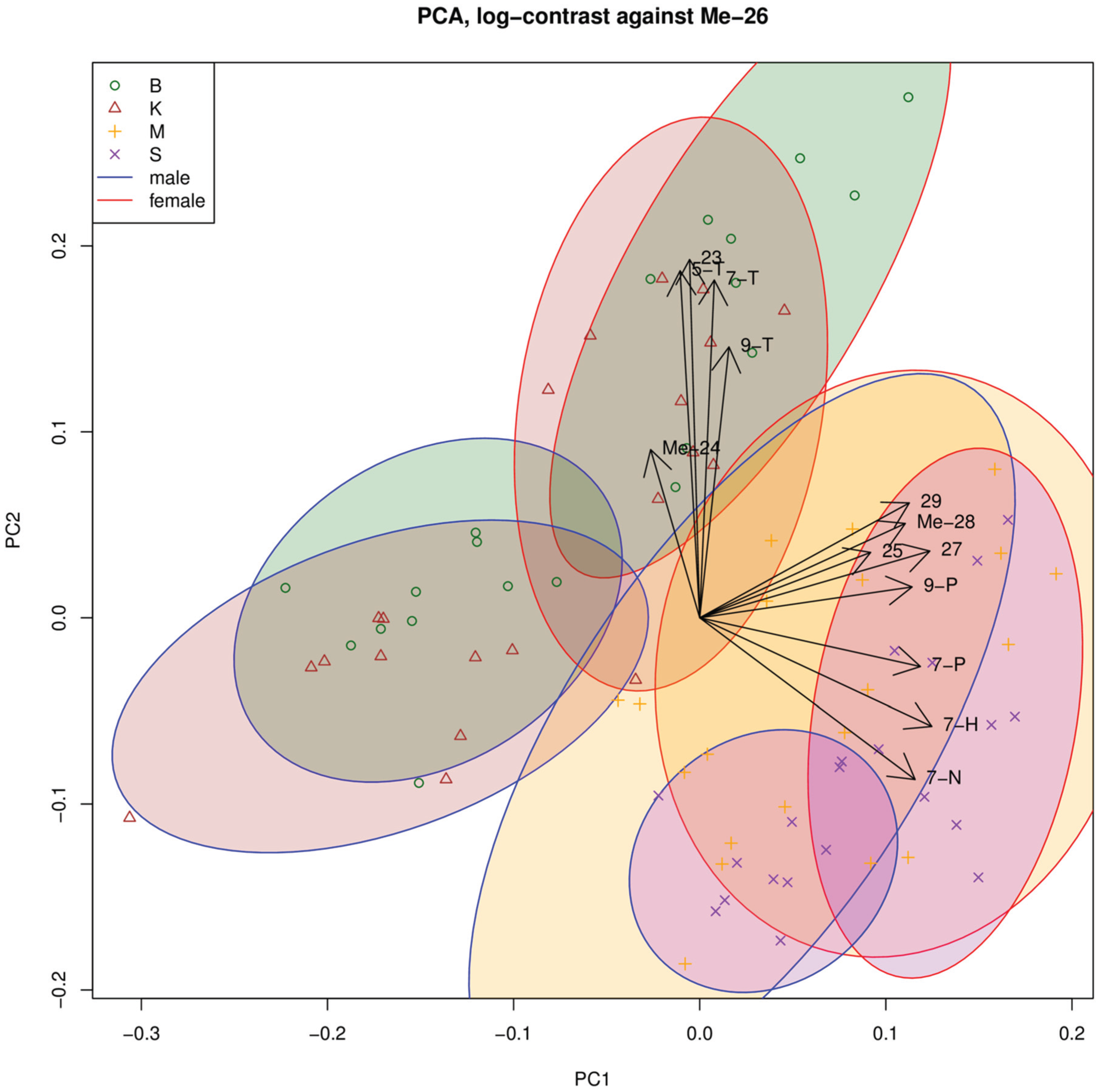
Table 2. Principal component analysis of the CHC composition in each population separated the values according to (7-H, 7-P, 9-P, 7-N, 25:0, 27:0, 29:0, Me-28) for the first component and (7-T, 9-T, 23:0) for the second component (
Figure 1). As the second component contains the CHCs in C23, we wondered whether there was a difference in CHC chain length among the populations (
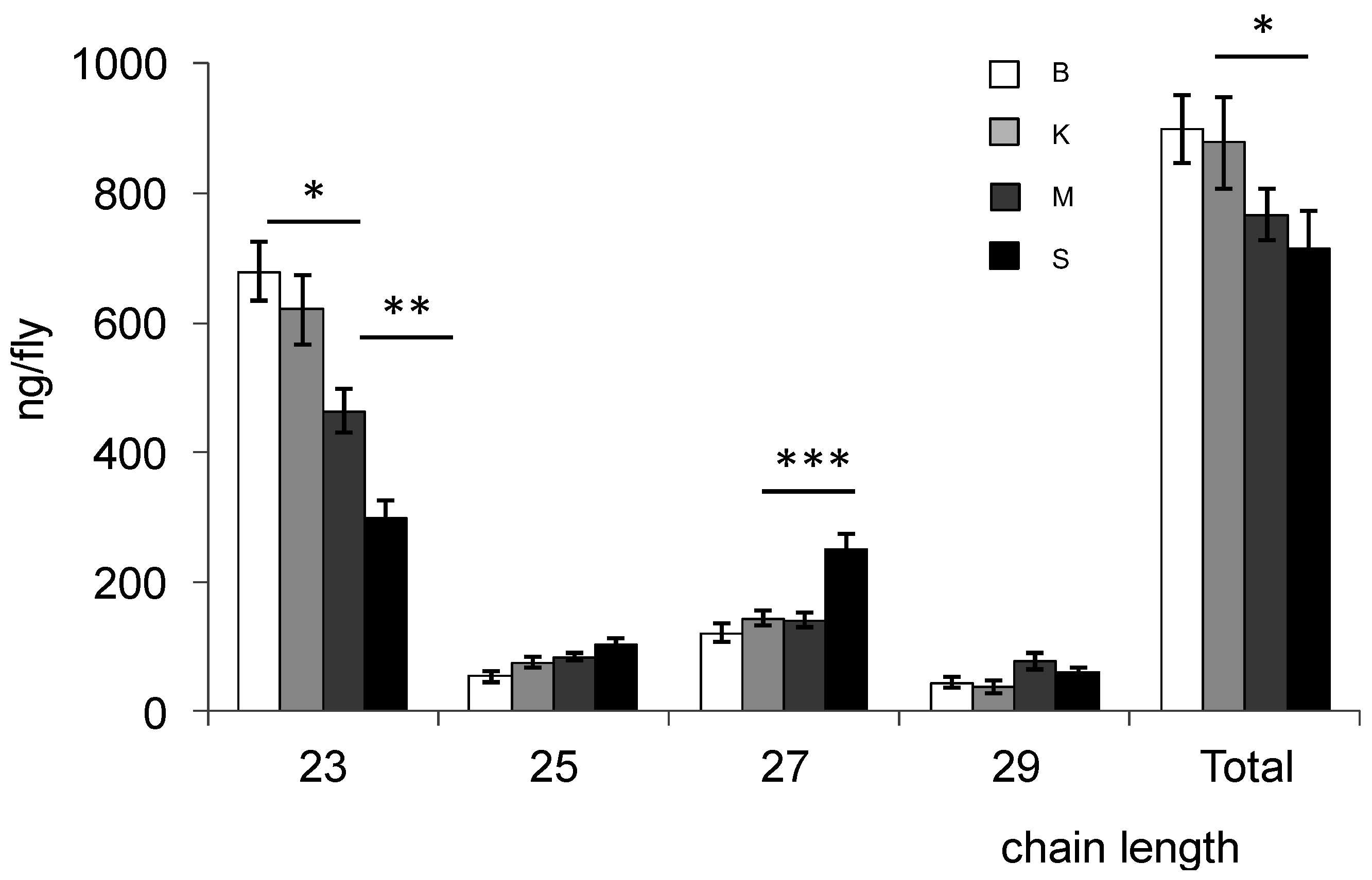
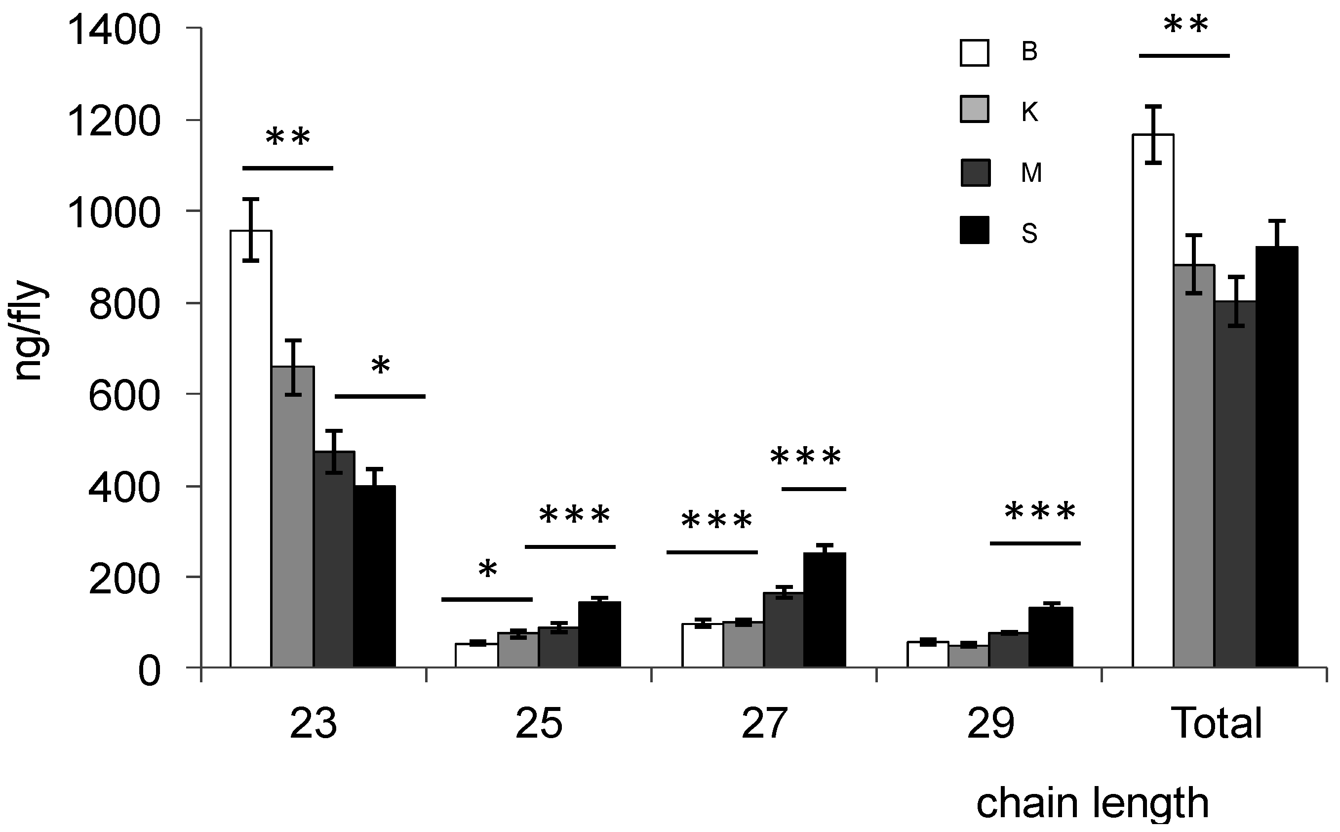
Figure 2). Bioko and Kounden males had the most CHCs (17% more than Mayotte and Sao-Tome males). The difference in C23 compounds was particularly large (8.6%, 31.6% and 55.8% less in Kounden, Mayotte, Sao-Tome males than in Bioko). Sao-Tome males had also two times more C27 than males from the other populations.
Table 1.
Male CHC profiles of four strains of D. yakuba.
Table 1.
Male CHC profiles of four strains of D. yakuba.
| CHC | Bioko | Kounden | Mayotte | Sao-Tome |
|---|
| 23–29 tot | 898.9 ± 52.1 | 877.8 ± 71.8 | 766.3 ± 125.6 | 714.7 ± 58.4 |
| 9-T | 2.17 ± 0.17 | 5.27 ± 1.04 | 4.36 ± 1.04 | 3.69 ± 0.89 |
| 7-T | 57.51 ± 2.84 | 48.56 ± 1.97 | 45.95 ± 1.74 | 27.90 ± 1.82 |
| 5-T | 1.20 ± 0.09 | 1.61 ± 0.14 | 0.94 ± 0.13 | 1.04 ± 0.12 |
| 23:0 | 14.48 ± 0.73 | 14.41 ± 0.63 | 8.21 ± 0.58 | 9.13 ± 0.54 |
| Me-24 | 0.98 ± 0.12 | 1.19 ± 0.11 | 0.53 ± 0.17 | 0.92 ± 0.10 |
| 9-P | 0.36 ± 0.06 | 0.67 ± 0.08 | 1.43 ± 0.13 | 1.52 ± 0.11 |
| 7-P | 1.19 ± 0.14 | 2.82 ± 0.25 | 4.84 ± 0.40 | 5.91 ± 0.27 |
| 25:0 | 3.43 ± 0.80 | 3.79 ± 0.43 | 4.24 ± 0.48 | 5.88 ± 0.47 |
| Me-26 | 10.61 ± 0.85 | 14.37 ± 0.53 | 11.54 ± 1.04 | 14.04 ± 0.48 |
| 7-H | 0.49 ± 0.06 | 0.19 ± 0.05 | 3.66 ± 0.49 | 15.90 ± 1.41 |
| 27:0 | 2.44 ± 0.66 | 1.97 ± 0.39 | 3.67 ± 0.35 | 4.64 ± 0.34 |
| Me-28 | 4.34 ± 0.61 | 3.90 ± 0.93 | 8.73 ± 1.09 | 4.23 ± 0.47 |
| 7-N | 0.0 ± 0.0 | 0.04 ± 0.04 | 0.28 ± 0.07 | 3.84 ± 0.61 |
| 29:0 | 0.42 ± 0.12 | 0.49 ± 0.12 | 0.81 ± 0.12 | 0.66 ± 0.11 |
Table 2.
Female CHC profiles of four strains of D. yakuba.
Table 2.
Female CHC profiles of four strains of D. yakuba.
| CHC | Bioko | Kounden | Mayotte | Sao-Tome |
|---|
| 23–29 tot | 1168.8 ± 61.4 | 883.2 ± 64.7 | 803.9 ± 53.6 | 921.1 ± 56.0 |
| 9-T | 3.08 ± 0.26 | 9.69 ± 1.34 | 3.89 ± 0.99 | 2.91 ± 0.62 |
| 7-T | 58.94 ± 1.61 | 46.46 ± 2.62 | 46.11 ± 1.78 | 28.13 ± 2.18 |
| 5-T | 1.44 ± 0.14 | 2.41 ± 0.44 | 0.74 ± 0.10 | 0.85 ± 0.14 |
| 23:0 | 17.65 ± 0.42 | 14.44 ± 0.92 | 6.69 ± 0.77 | 10.28 ± 0.84 |
| Me-24 | 0.41 ± 0.05 | 0.97 ± 0.18 | 0.41 ± 0.05 | 0.82 ± 0.17 |
| 9-P | 0.43 ± 0.04 | 1.28 ± 0.19 | 2.30 ± 0.30 | 2.01 ± 0.09 |
| 7-P | 1.09 ± 0.06 | 2.70 ± 0.35 | 5.29 ± 0.60 | 7.50 ± 0.42 |
| 25:0 | 2.92 ± 0.56 | 3.56 ± 0.43 | 3.01 ± 0.29 | 5.11 ± 0.41 |
| Me-26 | 4.82 ± 0.57 | 8.14 ± 0.83 | 8.14 ± 0.61 | 9.13 ± 0.47 |
| 7-H | 0.77 ± 0.06 | 0.60 ± 0.11 | 6.48 ± 0.97 | 11.98 ± 0.64 |
| 27:0 | 3.10 ± 0.39 | 3.00 ± 0.35 | 6.57 ± 0.81 | 6.11 ± 0.63 |
| Me-28 | 4.26 ± 0.51 | 5.29 ± 0.53 | 8.01 ± 0.50 | 7.22 ± 0.87 |
| 7-N | 0.04 ± 0.02 | 0.04 ± 0.03 | 0.62 ± 0.13 | 5.56 ± 0.53 |
| 29:0 | 0.77 ± 0.10 | 0.56 ± 0.09 | 1.19 ± 0.15 | 1.56 ± 0.21 |
Figure 1.
Principal component analysis of CHC compositions in the different populations. Bioko (B), Kounden (K), Mayotte (M), Sao-Tome (S).
Figure 1.
Principal component analysis of CHC compositions in the different populations. Bioko (B), Kounden (K), Mayotte (M), Sao-Tome (S).
Figure 2.
Amount of hydrocarbons of different lengths extracted from male (top) and female (bottom) D. yakuba flies from Bioko (B), Kounden (K), Mayotte (M) and Sao-Tome (S) populations. Total: C23 to C29; Each bar represents mean ± SEM (n = 10). *, ** and *** above bars indicate significant differences (one-way ANOVA, p = 0.05, 0.01 and 0.001, respectively) between means.
Females from Bioko had the most CHCs (35% more than females from the other populations). There was also a large discrepancy in the amount of C23 (31.3%, 50.7% and 58.6% less in Kounden, Mayotte, Sao-Tome females than in Bioko). Sao-Tome females had the most C25, C27 and C29 (161.9%, 153.6% and 129.4% more than Bioko females).
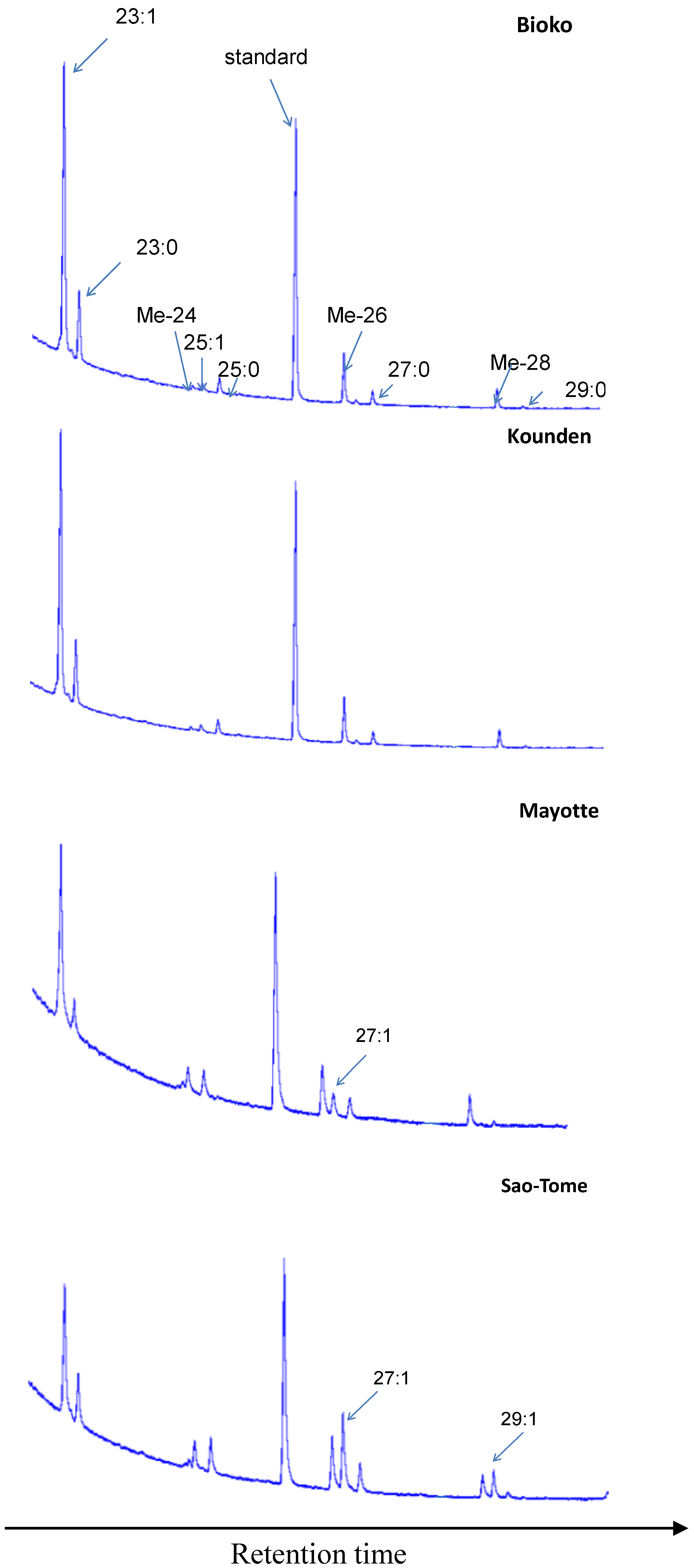
Figure 3 gives typical examples of male CHC chromatograms. The largest differences concerned 7-H, and 7-N:7-H represents about 16% of the CHCs in Sao-Tome, and only 0.5% in Bioko. 7-N represents 4% of the CHCs in Sao-Tome, but is barely detectable in Kounden and Mayotte and is absent in Bioko.
3.2. Mating Behavior and Mate Discrimination between Strains
Bioko males more often exhibited courtship and eventually mated than did males from the other populations. Around 50%, of Kounden, Mayotte and Sao-Tome males mated—about 28% less than Bioko (
Table 3). Latency times were high and somewhat higher for Mayotte and Sao-Tome (around 24 min) than for Kounden (around 18 min). Copulation duration did not differ significantly among populations.
Table 3.
Mating behavior parameters of D. yakuba strains.
Table 3.
Mating behavior parameters of D. yakuba strains.
| Population | Total Number | Copulation Percentage | n | Copulation Latency | Duration of Copulation |
|---|
| Bioko | 50 | 70 | 35 | 21.56 ± 1.14 ab | 41.50 ± 1.35 a |
| Kounden | 51 | 60.78 | 31 | 18.03 ± 1.07 b | 38.81 ± 1.72 a |
| Mayotte | 54 | 51.85 | 28 | 24.14 ± 1.61 a | 36.19 ± 2.15 a |
| Sao-Tome | 62 | 50 | 31 | 24.53 ± 0.86 a | 40.95 ± 1.67 a |
Figure 3.
Gas chromatograms of D. yakuba males. 23:1 (tricosenes), 23:0 (tricosane), Me-24 (2-methyltetracosane), 25:1 (pentacosenes), 25:0 (pentacosane), standard (hexacosane), Me-26 (2-methylhexacosane), 27:1 (7-heptacosene), 27:0 (heptacosane), Me-28 (2-methyloctacosane), 29:1 (7-nonacosene), 29:0 (nonacosane).
All mating behavior experiments showed a significant departure from random mating, suggesting partial reproductive isolation (253 homogeneous pairs
vs. 177 heterogeneous,
p-value < 0.001 in the 1 female/2 male experiment; 219
vs. 145 pairs,
p-value < 0.001 in the 1 male/2 female experiment; and 126
vs. 67 pairs,
p-value < 0.001 in the 2 males/2 females experiment) (
Table 4,
Table 5 and
Table 6).
Table 4.
Female-choice experiment (1 female/2 males). The three categories were: homogeneous crosses, (Hom), heterogeneous crosses (Het), and no mating. Departure from the random mating hypothesis (H0A: as many homogeneous as heterogeneous crosses) was quantified using the bilateral binomial p-value. Multiple testing-corrected p-values (Holm-Bonferroni correction) are indicated as p*; B: Bioko; K: Kounden; M: Mayotte; S: Sao-Tome.
| Female | Male | Hom | Het | No Mating | p (H0A) | p* (H0A) |
|---|
| B | K | 21 | 17 | 8 | 0.627 | 1.000 |
| B | M | 20 | 14 | 3 | 0.392 | 1.000 |
| B | S | 17 | 20 | 5 | 0.743 | 1.000 |
| K | B | 25 | 27 | 2 | 0.890 | 1.000 |
| K | M | 18 | 20 | 9 | 0.871 | 1.000 |
| K | S | 21 | 11 | 18 | 0.110 | 0.992 |
| M | B | 22 | 13 | 8 | 0.175 | 1.000 |
| M | K | 23 | 11 | 18 | 0.058 | 0.576 |
| M | S | 17 | 13 | 14 | 0.585 | 1.000 |
| S | B | 23 | 7 | 18 | 0.005 | 0.057 |
| S | K | 28 | 7 | 11 | 0.001 | 0.006 |
| S | M | 18 | 17 | 11 | 1.000 | 1.000 |
Table 5.
Male choice experiment (1 male/2 females). See
Table 4 for descriptions of categories.
Table 5.
Male choice experiment (1 male/2 females). See Table 4 for descriptions of categories.
| Male | Female | Hom | Het | No Mating | p (H0A) | p* (H0A) |
|---|
| B | K | 16 | 14 | 3 | 0.856 | 1.000 |
| B | M | 21 | 10 | 6 | 0.071 | 0.637 |
| B | S | 23 | 8 | 19 | 0.011 | 0.117 |
| K | B | 10 | 9 | 6 | 1.000 | 1.000 |
| K | M | 25 | 20 | 17 | 0.551 | 1.000 |
| K | S | 28 | 8 | 19 | 0.001 | 0.014 |
| M | B | 16 | 15 | 3 | 1.000 | 1.000 |
| M | K | 9 | 11 | 6 | 0.824 | 1.000 |
| M | S | 13 | 14 | 10 | 1.000 | 1.000 |
| S | B | 17 | 16 | 7 | 1.000 | 1.000 |
| S | K | 17 | 9 | 4 | 0.169 | 1.000 |
| S | M | 24 | 11 | 9 | 0.041 | 0.410 |
Table 6.
Multiple choice experiment (2 males/2 females). The four categories were: Hom 1: Homogeneous for population 1 (Hom 1), homogeneous for population 2 (Hom 2), heterogeneous (Het), and no mating (no). For each experiment, we tested three hypotheses (H0A: equal homogeneous and heterogeneous crosses, H0B: equal homogeneous crosses of each kind, H0C: random mating, which means 25% of each homogeneous cross and 50% heterogeneous crosses).
| Pop 1 | Pop 2 | Hom 1 | Hom 2 | Het | No | p (H0A) | p* (H0B) | p (H0B) | p* (H0B) | p (H0C) | p* (H0C) |
|---|
| B | K | 8 | 5 | 18 | 5 | 0.482 | 0.964 | 0.569 | 1.000 | 0.498 | 0.498 |
| B | M | 14 | 9 | 12 | 5 | 0.097 | 0.388 | 0.417 | 1.000 | 0.102 | 0.408 |
| K | M | 13 | 15 | 10 | 2 | 0.003 | 0.018 | 0.843 | 1.000 | 0.016 | 0.096 |
| B | S | 4 | 14 | 17 | 2 | 1.000 | 1.000 | 0.028 | 0.168 | 0.066 | 0.330 |
| K | S | 10 | 12 | 12 | 6 | 0.114 | 0.388 | 0.831 | 1.000 | 0.222 | 0.444 |
| M | S | 10 | 12 | 11 | 6 | 0.073 | 0.365 | 0.836 | 1.000 | 0.146 | 0.438 |
In the female choice experiment (
Table 4), the analysis of deviance identified a significant effect of the female population on the proportion of homogeneous pairs (
p = 0.04), but no effect of the male population (
p = 0.32). The GLM with no intercept (test for the departure from random mating) attributes this effect to females from the Mayotte population (
p = 0.01) and from the Sao-Tome population (
p < 0.001), while Bioko and Kounden females seem to mate randomly (
p = 0.50 and
p = 0.59, respectively). There was also a significant female effect on the proportion of non-mating events (
p = 0.002 in the analysis of deviance). Females from populations Bioko and Kounden mated more often than females from populations Mayotte and Sao-Tome. We found no significant effect from population on copulation latency for either females (
p = 0.06) or males (
p = 0.64).
In the male choice experiment, we found no evidence of a differential effect of male (p = 0.13 in the analysis of deviance) or female (p = 0.16) population on the proportion of homogeneous crosses, although some specific crosses (such as Kounden male × Sao-Tome female) departed significantly from random mating hypothesis on their own. In contrast, there was a significant effect of female population on the proportion of pairs in which there was no mating (p = 0.009)—an effect that was not observed for males (p = 0.11). More specifically, the GLM identified a significant departure of females from the Sao-Tome population (p = 0.0028) compared to the Bioko population, which was taken arbitrarily as a reference. This strongly suggests that the presence of a Sao-Tome female in the experiment prevented any male from another population from mating with the other female. We found no significant effect of male (p = 0.46) or female (p = 0.05) population on copulation latency.
In the multiple-choice test, testing for random mating is more complicated as there can be deviations from the 1:1 ratio of homogeneous/heterogeneous crosses and/or uneven frequencies of homogeneous crosses. A binomial GLM with no intercept showed that only the Mayotte population had a significant influence on the excess of homogeneous crosses (p = 0.002). In contrast, Sao-Tome and Bioko populations were the only ones driving a significant deviation from an even representation of both kinds of homogeneous pairs (4 Bioko-Bioko pairs vs. 14 Sao-Tome-Sao-Tome pairs, p = 0.027). Sao-Tome population showed a general trend towards being preferentially associated with such deviations, but this average effect was not significant (p = 0.057). We did not detect any population effect on copulation latency or on the proportion of pairs in which there were no mating events.


