Abstract
Description of flow stress evolution, specifically an approximation of a set of flow curves acquired under a wide range of thermomechanical conditions, of various materials is often solved via so-called flow stress models. Some of these models are associated with a description of significant flow-curve coordinates. It is clear, the more accurate the coordinates description, the more accurate the assembled model. In the presented research, Zener–Hollomon-based relations, multi-layer perceptron networks and multivariate polynomials are employed to describe the peak and steady-state coordinates of an Invar 36 flow curve dataset. Comparison of the utilized methods in the case of the studied alloy has showed that the suitable description is given by the multivariate polynomials although the Zener–Hollomon and perceptron networks also offer valuable results.
1. Introduction
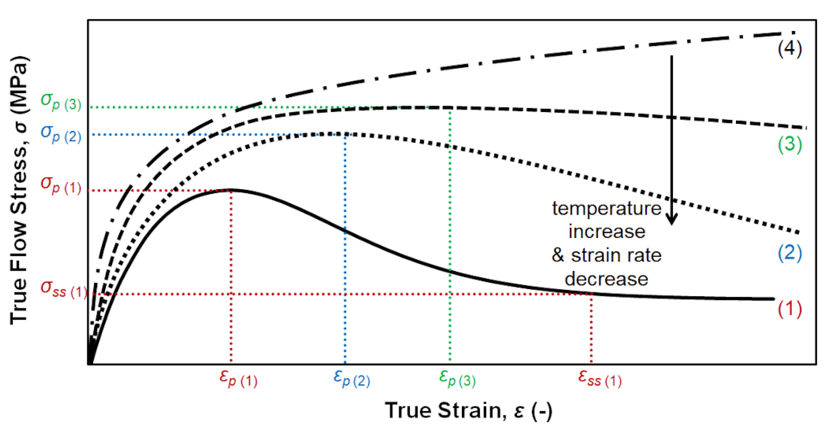
Since the beginning of the 20th century, so-called flow stress models have been being utilized for the mathematical description of experimentally gained cold and hot flow-curve datasets of various steels and other intended-to-forming materials [1]. As a consequence of softening phenomena accompanying hot deformation (i.e., a dynamic recovery and especially a dynamic recrystallization), the description of hot flow stress evolution under different thermomechanical conditions (i.e., strain, strain rate, and temperature levels) is associated with an issue of different flow curve shapes which can be at the same time presented in the frame of a single experimental dataset [1,2]—see Figure 1 for illustration. In an effort to cope with this issue, numerous models with a various mathematical structure have been proposed and tested on the hot flow curve datasets of countless materials—see e.g., [3,4,5,6,7,8,9,10,11,12,13,14,15,16,17,18,19,20]. Based on the previously published works, the Cingara and McQueen’s relationship [5] and JMAK-theory-based model [9] belong among the easy-to-assembly and often-used ones, and by-strain compensated Garofalo’s hyperbolic-sine equation (SCG) [7] can be then considered as the most frequently utilized one. Further, it is also possible to encounter on, e.g., Ebrahimi’s relation [6], Fields–Backofen [3], Johnson–Cook [4], and Hensel–Spittel [21] models or a series of Solhjoo’s equations [22,23,24,25,26,27], etc. From time to time, efforts to modify the proposed models and thus enhance their approximation accuracy are also noticed—see e.g., a modification of the Hensel–Spittel model [28], modifications in the Fields–Backofen model [29,30], Johnson–Cook modification [18,31], an enhancement of the SCG model [32,33], or improvements in the Cingara and McQueen’s relationship [34]. In addition, so-called visco-plastic constitutive models are also object of interest—see e.g., Anand’s relation [35,36] or Kozlowski’s model [36,37]. In the last years, it is also possible to come across with a so-called artificial-neural-network (ANN) approach of flow curve approximation—either as a pure ANN methodology [38,39,40,41,42,43,44,45] or in combination with the proposed flow stress models (hybrid methods) [46,47]. These ANN approaches are mainly based either on using of multi-layer perceptron architecture with the classic back-propagation learning algorithm (see e.g., [38,39,40,42]) or on employing of deep learning techniques (see e.g., [41,44,45]). Moreover, improving of flow stress modeling via so-called metamodels in the form of Kriging approximation and artificial neural network have also been studied—see [48,49].
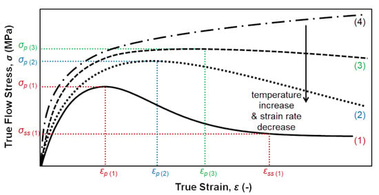
Figure 1.
Influence of thermomechanical conditions on the flow stress course and position of the significant flow-curve points. The coordinates of the significant points, specifically the peak strain, peak stress, steady-state strain, and steady-state stress are labelled as εp (-), σp (MPa), εss (-) and σss (MPa), respectively.
However, all above introduced methods encounter at the pursuit on flow stress description on various difficulties. For instance, the mentioned ANN approach requires sufficiently large dataset because of overtraining issue. Note, in order to overcome the overtraining issue and thus perform a successful and meaningful prediction via the ANN approach, a flow curve dataset have to be divided into the training part (to learn the network) and testing part (to verify the prediction capability out of the experimental conditions) [38,39,40,41,42,43]. Accuracy of the SCG model is strongly influenced by the complicated dependency of the parameters of the Garofalo’s relationship on the strain level [7,8,10,12]. An accuracy of numerous models (e.g., Cingara-McQueen, JMAK, Ebrahimi or Solhjoo) is then highly influenced by an accuracy of a peak and steady-state description—see the coordinates of the significant flow-curve points in Figure 1, especially εp (-), σp (MPa) and σss (MPa). This description is most frequently performed via the power-law and/or inverse hyperbolic sine dependency on the Zener–Hollomon parameter [50], see e.g., [6,11,12,15,22,23,51]—however, this can be insufficient if the experimentally acquired coordinates don’t fit into these trends. Nevertheless, alternatives can be found in order to describe the peak point coordinates and steady-state stress coordinate more precisely—see, e.g., interpolation and closed-form functions in [52] or an ANN approach in [47].
From a practical point of view, the assembled flow stress models are sometimes implemented into the FEM (Finite Element Methods) simulation software in order to model a course of real hot forming processes [1]. An accurate FEM simulation requires large number of flow stress data in a wide range of thermomechanical conditions [39]. Flow stress prediction techniques are usually utilized for this purpose (see FEM simulations, e.g., in [38,39]) since an experimental acquiring of large dataset is time-consuming and costs-increasing issue [39]. It is clear that an accuracy of the utilized flow stress description has a significant impact on the FEM simulation results—techniques of accuracy improving are thus of high interest [1,39]. Moreover, as previously published, an accuracy of flow stress models can find its practical application also in the case of an assembling of so-called processing maps—see e.g., [38,42].
In frame of the submitted research, experimentally obtained coordinates of the peak point and steady-state stress of an Invar 36 (FeNi36) alloy (also known as Dilaton 36) are approximated via three different approaches (based on the Zener–Hollomon parameter, ANN approach and bivariate polynomials) and inserted into the Cingara-McQueen and JMAK-theory-based models. The aims are to assembly an as accurate as possible description of the experimental hot flow curve dataset of the Invar 36 alloy and in the same time demonstrate and compare various approaches for the peak point and steady-state stress description.
2. Materials and Methods
2.1. Acquiring of Experimental Hot Flow Curve Dataset
The cylindrical samples of the Invar 36 (FeNi36) alloy with a diameter of 10 mm and a length of 15 mm were subjected to uniaxial hot compression testing by means of the Gleeble 3800 Thermal-Mechanical Simulator with its Hydrawedge II Mobile Conversion Unit (Dynamic Systems Inc., Poestenkill, NY, USA) [53]. The testing has been performed for a combination of four deformation temperatures (1173, 1273, 1393, and 1523 K) with three strain rates (0.01, 0.3, and 10 s−1). Each tested sample was preheated to a specific deformation temperature by a heating rate of 5 K·s−1 (mediated via a direct electric resistance heating), subsequently held on this temperature for a dwell time of 120 s and then immediately compressed to a true strain of 1.0. The temperature was measured by a pair of thermocouple wires of K-type, i.e., Ni-Cr (+) and Ni-Al (−), which were fixed by a welding in the middle length of a tested sample. Tantalum foils and nickel-based grease were applied in order to protect the anvils and reduce a friction on the anvils–sample interface. In addition, in order to inhibit oxidation processes, the testing chamber was during the test course held under vacuum. The experimental process resulted in a set of twelve flow curves of the investigated alloy.
2.2. Flow Curve Description
In frame of this research, the well-known Cingara and McQueen’s relationship [5] has been utilized in order to describe the experimentally obtained flow curve dataset in the before-the-peak strain range, i.e., ε ≤ εp (see the first part of Equation (1)). The description has been thereafter completed via the Kolmogorov’s relation [54] (studied also by Johnson, Mehl, and Avrami—known as JMAK [55]) modified to describe the beyond-the-peak region, i.e., ε ≥ εp [9] (the second part of Equation (1)):
In Equation (1), σ (MPa) and ε (-) represent the values of true stress and true strain, respectively. The p and s subscripts then correspond with the peak and steady-state coordinates, respectively. Taking the experimental values of σ and ε, including the peak and steady state coordinates, the experimental values of the c-parameter (-) were calculated on the basis of the least squares method (LSM) [56] as the slope of the line of ln(σ/σp) vs. ln(ε/εp) + 1 − ε/εp, always at a constant temperature and strain rate. The experimental values of the n (-) and k (-) parameters were obtained from the slope of the line and intercept of ln{ln[(σp − σss)/(σ − σss)]} vs. ln(ε/εp − 1), also for a constant temperature and strain rate. The approximation of these curve-shape-control parameters has been realized via the following formula [57]:
where T (K) and (s−1) are a deformation temperature and strain rate, respectively. The material constants a1 (-), a2 (-), a3 (K), and a4 (K−1) have been estimated individually for each parameter by nonlinear least squares method (NLSM) via the Levenberg–Marquardt (LM) optimization algorithm [58,59,60].
2.2.1. Peak and Steady-State Description via Zener–Hollomon Parameter
The experimental values of the peak point coordinates (the peak strain εp and peak stress σp) and the steady-state stress σss (i.e., three vectors, each with twelve datapoints) have been described with respect to the change in a temperature and strain rate level via three approaches. The first one is based on a utilizing of the well-known Zener–Hollomon parameter, Z (s−1) [50]:
where Q (J·mol−1) and R (8.314 J·K−1·mol−1) represent an apparent activation energy and universal gas constant, respectively. Considering the Z-parameter, the above-mentioned flow-curve coordinates have been described as follows [20,51]:
The values of the activation energy, Q, and other material constants in Equation (5), i.e., A (s−1), n (-) and α (MPa−1), were obtained on the basis of regression analysis of the Garofalo’s relation [61]:
where σ (MPa) represents the values of σp or σss. A rough estimate of the material constants of the Equation (6) have been obtained as described in [20,51] and subsequently refined via the LM optimization algorithm [58,59,60]. The material constants a (s) and b (-) were then calculated on the basis of LSM method [56] from the slope of the line and intercept of ln(εp) vs. ln(Z).
2.2.2. Peak and Steady-State Description via Multi-Layer Perceptron Network
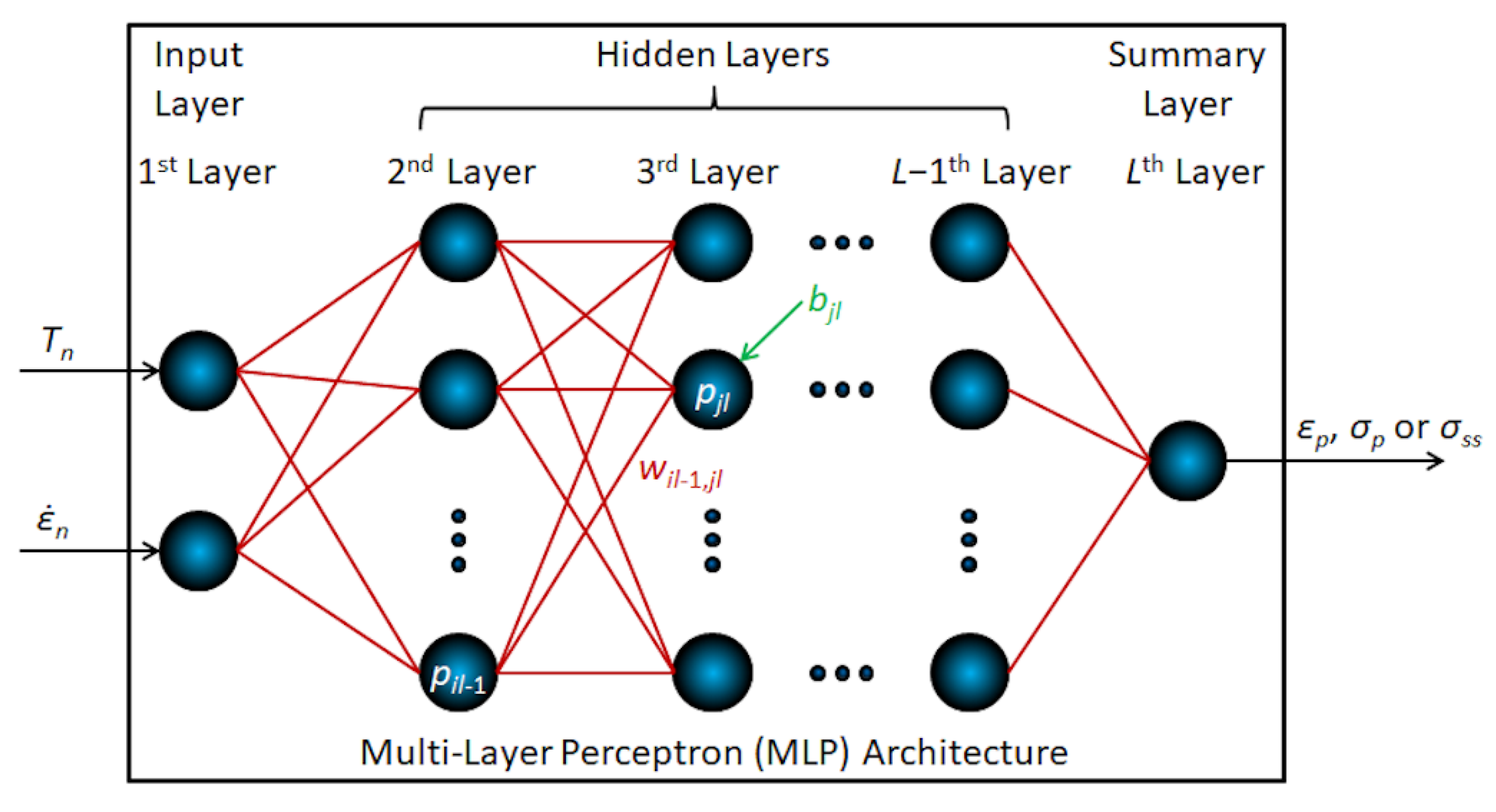
The second approach [47] deals with a utilizing of three individually-customized Multi-Layer Perceptron (MLP) networks, i.e., ANN methodology [62,63]. The general scheme of the utilized MPL networks is given in Figure 2.
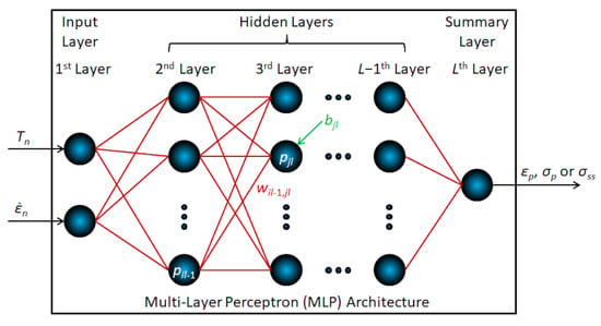
Figure 2.
General architecture of the utilized multi-layer perceptron networks. The blue-black spheres—artificial neurons (perceptrons); The red lines—synaptic connections.
Input information (vectors of independent variables) is inside the MLP architecture processed by individual computational units (perceptrons), clustered into the layers communicating via synaptic weights, and corresponding output information (vector of dependent variable) is subsequently returned. Each perceptron of the hidden or summary layer is in accordance with the scheme in Figure 2 mathematically formulated as follows [64]:
In Equation (7), pil−1 is the vector of i-th perceptron of l−1-th layer, pjl and bjl are the vector and bias of j-th perceptron of l-th layer, wil−1,jl is a synaptic weight connecting the perceptrons pil−1 and pjl, φ is then the perceptron activation function. Note, i = [1, I] ⊂ ℕ, j = [1, J] ⊂ ℕ, and l = [2, L] ⊂ ℕ, where I and J are number of perceptrons in the l−1-th and l-th layer, respectively and L is then overall number of layers. Perceptrons of the input layer are equal to the normalized vectors of temperature, Tn (-), and strain rate, (-). Normalization procedure has been performed via method described in [42].
The specific architectures of the MLP network suitable for the description of the individual flow curve coordinates have been established on the basis of an adaptation and learning procedures (analogical procedures were described previously in [42]).
As mentioned in the introduction, a learning procedure can be done via various methods. Based on the previous experiences [42,47] and some other published papers [38,39,40], the learning procedure was performed by a minimization of a mean squared error [65] (performance function) via a combination of the LM algorithm [58,59,60] with the Bayesian regularization [66,67] under the back-propagation of error signal [68]. The experimental dataset contains twelve flow curves—i.e., twelve experimental data-rows for each described parameter (εp, σp and σss). Note, 1/6 (i.e., two data-rows: 1523 K/10 s−1 and 1173 K/0.3 s−1) were always used for the cross validation during the learning course, 1/3 (four data-rows: 1393 K/0.01 s−1, 1393 K/0.3 s−1, 1273 K/0.01 s−1, and 1273 K/10 s−1) were chosen for an evaluation of prediction capability (a testing of possible overtraining issue) after the learning procedure and the rest of the dataset (1/2, i.e., six data-rows) was directly subjected to the minimization algorithm.
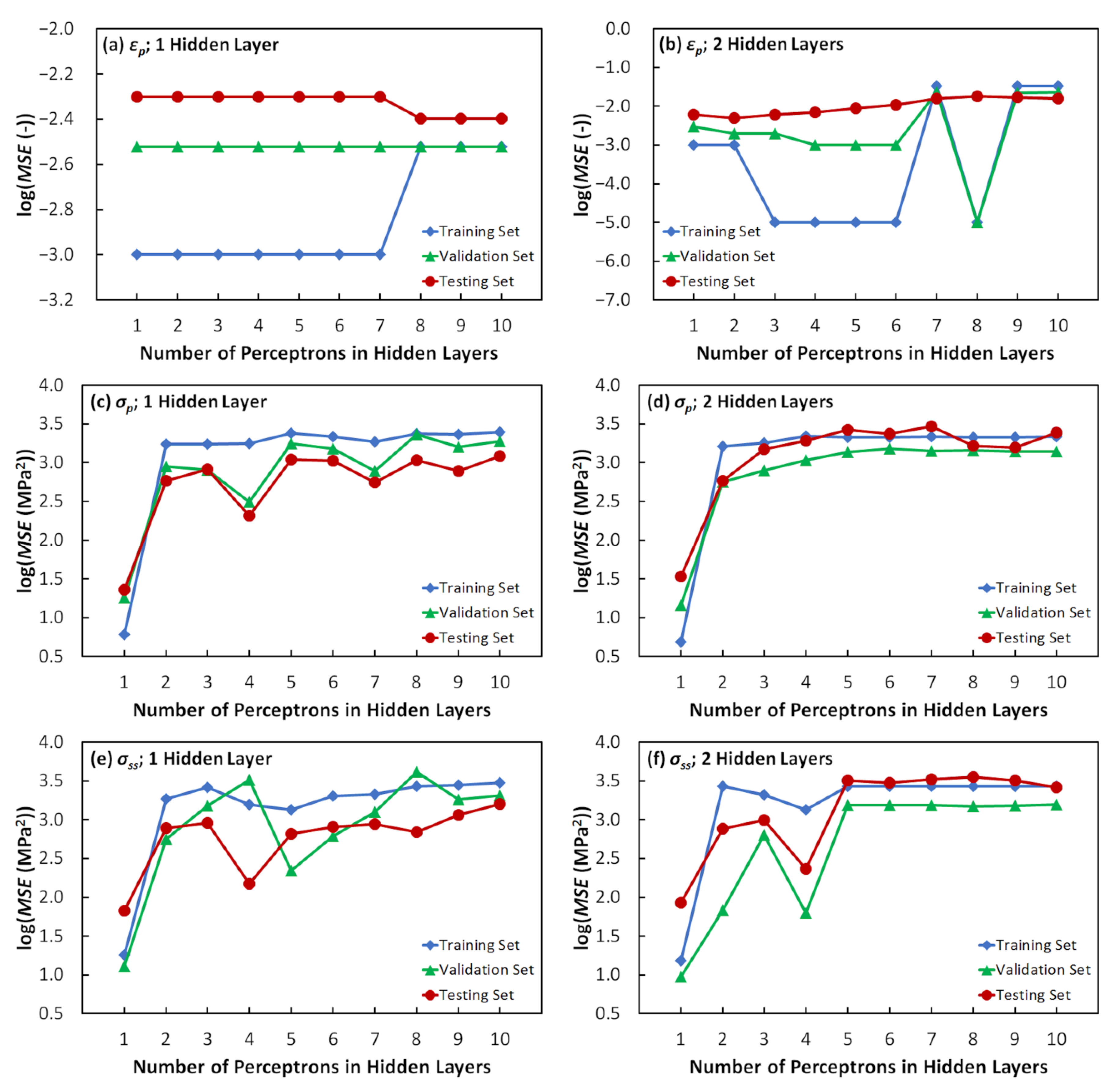
Detailed course of the adaptation procedure, i.e., finding of an appropriate network architecture, is graphically expressed in Figure 3. As above-mentioned, a Mean Squared Error, MSE (-, MPa) [65], has been employed as a performance function:
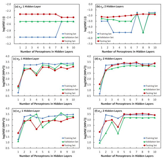
Figure 3.
An influence of network architecture on a value of mean squared error. (a) Peak strain description—1 hidden layer; (b) peak strain description—2 hidden layers; (c) peak stress description—1 hidden layer; (d) peak stress description—2 hidden layers; (e) steady-state stress description—1 hidden layer; (f) steady-state stress description—2 hidden layers.
In this equation, the Ti (-, MPa) and Ai (-, MPa) embody the values of the target (i.e., experimental) and approximated vectors of the specific flow curve coordinate, respectively. The i = [1, n] ⊂ ℕ, where the n is the number of elements in the training, validation or testing dataset. The charts in Figure 3 clearly demonstrate an influence of number of hidden layers and perceptrons on a MSE-value. With respect to the εp-description under 1 hidden layer (Figure 3a), it can be seen that the MSE-values of the training and testing set remain practically unchanged (constant) until a number of hidden perceptrons is equal to seven. After a small change under eight perceptrons, the MSE-values are constant again. Note, the MSE-value of the validation set remains unchanged despite of number of hidden perceptrons. As can be seen, the MSE-values of the testing set are always the highest—the network is under one hidden layer overtrained and thus not appropriate. Two hidden layers (Figure 3b) show more complicated trends—especially with respect to the training and validation set. It can be seen, the network is not overtrained only under 7, 9, and 10 hidden perceptrons. However, the MSE-values of the training and validation set are in these cases higher than under others number of perceptrons. The network is then highly overtrained and thus unusable under 3–6 and 8 perceptrons. The overtraining under 1 and 2 perceptrons can be considered as negligible and the MSE-values of the training and validation set are satisfying. Finally, based on these results, an architecture with two hidden layers and two perceptrons inside has been selected as the appropriate one. The MSE-values of the σp and σss description share practically almost the same trend (see Figure 3c–f). A compromise between an overtraining and the enormously high MSE-values had to be done—so an architecture with one hidden layer and one hidden perceptron has been selected in the case of description of these stress parameters. A clear overview of all selected network architectures is demonstrated in Table 1.

Table 1.
Architecture features of adapted Multi-Layer Perceptron (MLP) networks.
The above described MLP networks were assembled and applied in the MATLAB® 9.3 environment [70] utilizing the Neural Network Toolbox™ 11.0 [71] (MathWorks®, Natick, MA, USA).
2.2.3. Peak and Steady-State Description via Multivariate Polynomials
The third approach is based on a utilizing of multivariate (specifically bivariate) polynomials [72]. The general form of the utilized polynomials is represented by the following formula:
The aij (-) are material constants, where the i = [0, n] ⊂ ℕ0 and j = [0, m] ⊂ ℕ0. It was found out that the appropriate approximation of the studied flow curve coordinates is given when the n = m = 3. The optimal values of the material constants, aij, have been for each coordinate obtained via the LM optimization algorithm [58,59,60].
3. Results and Discussion
3.1. Experimental Dataset
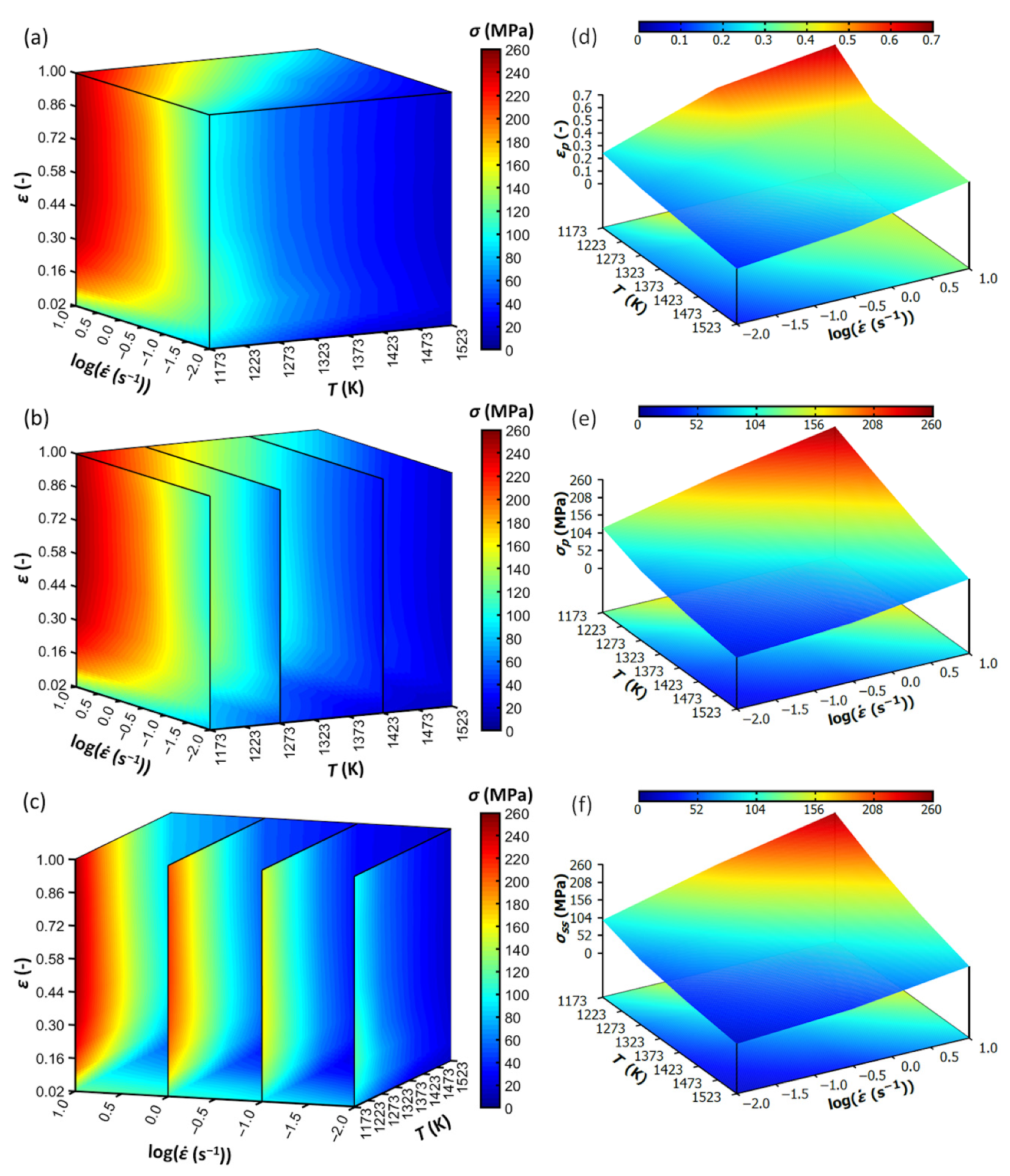
Figure 4 offers a graphical expression of the experimentally acquired data in the form of volumetric and surface charts as stated for an evolution of the flow stress and significant-flow-curve points, respectively. With respect to Figure 4a–c, the x, y, and z axes have been utilized to spatially express an interaction of the vectors of the independent variables, i.e., temperature, strain rate and strain, respectively. Their spatial intersections are then rendered as a 3D-color-space matrix representing the flow stress evolution. In order to visualize an influence of temperature and strain rate in more detail, the assembled volumetric expression is also offered in a form of sliced panels along the temperature and strain rate axes. As expected, a typical flow stress behavior can be observed—a flow stress level is moving downward as a temperature level increases and a strain rate level decreases. With respect to an increasing strain level, a flow stress firstly increases up to a peak point (a global maximum)—i.e., work hardening phase. After that, the flow stress either gently decreases (i.e., softening phase) with a subsequent transition to a steady-state phase or staying steady immediately. Figure 4d–f then expresses a characteristic impact of a mutual effect of temperature and strain rate on the position of the employed flow-curve coordinates (i.e., peak strain, peak stress, and steady-state stress). Predictably, all these coordinates decline with an increasing temperature level and decreasing strain rate level. It is noticeable, dependence of the peak and steady-state stress coordinates on the temperature and strain rate is in both cases expressed as a surface with a relatively simple curvature. A surface curvature of the peak strain dependence is then slightly complicated as regard to lower temperature levels—see the distinct breaks in the trend, i.e., a mathematical description can be in this case a little bit difficult. Figure 4a–c and Figure 4d–f have been constructed by means of the MATLAB® 9.3 software (MathWorks®, Natick, MA, USA) [70] and the Gnuplot 5.2 graphing utility Patchlevel 7 [73], respectively.
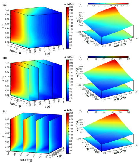
Figure 4.
Volumetric and surface expression of the experimental dataset of the studied alloy. (a) Flow stress evolution: Global overview; (b) flow stress evolution: Temperature axis detail; (c) flow stress evolution: Strain rate axis detail; (d) peak strain evolution; (e) peak stress evolution; and (f) steady-state stress evolution.
3.2. Evaluation of the Peak and Steady-State Description
The material constants of the above described peak and steady-state description approaches are shown in Table 2, Table 3, Table 4 and Table 5.

Table 2.
Material constants of the Zener–Hollomon based approach.

Table 3.
Material constants (weights and biases) of the MLP approach for the εp description.

Table 4.
Material constants (weights and biases) of the MLP approach for the σp and σss description.

Table 5.
Material constants of the multivariate-polynomial based approach.
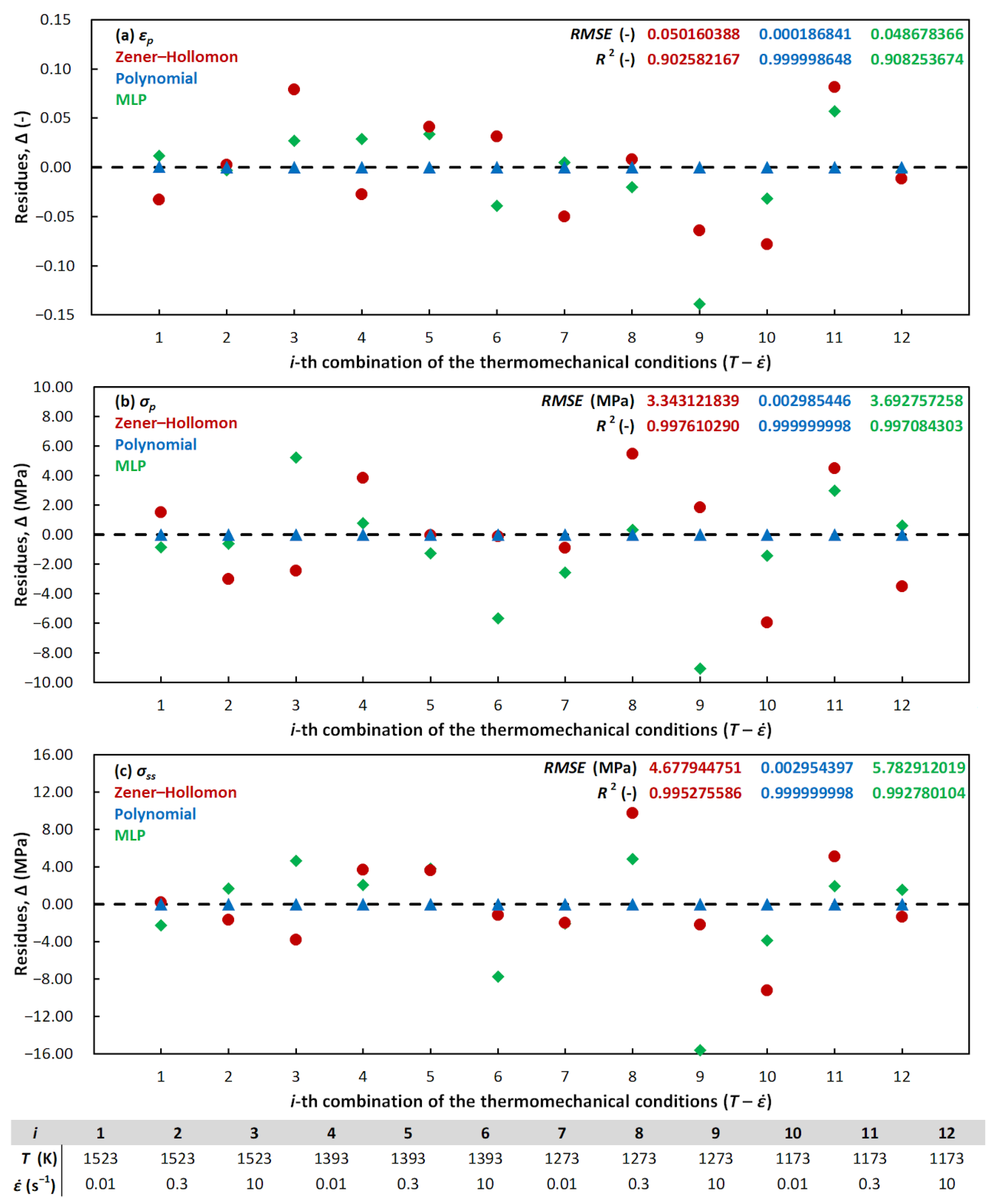
In order to compare the introduced approaches, residues, ∆ (-, MPa) (Equation (10)), Root Mean Squared Error, RMSE (-, MPa) [65] (Equation (11)), and determination coefficient, R2 (-) [74] (Equation (12)), have been employed—see Figure 5:
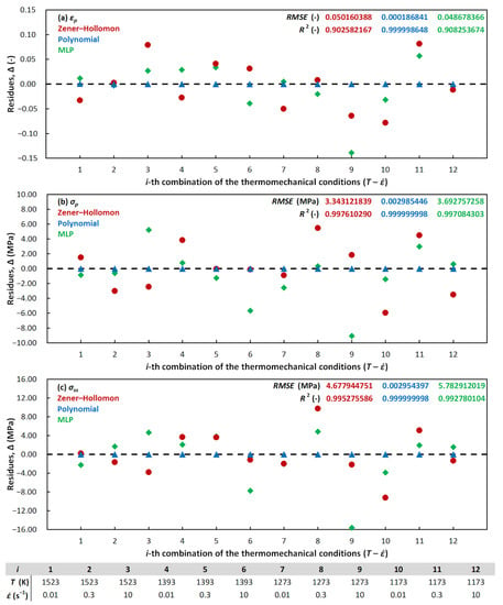
Figure 5.
Residues after the peak and steady-state approximation. (a) Peak strain approximation; (b) peak stress approximation; (c) steady-state stress approximation. The red circles—Zener–Hollomon approach; The blue triangles—multivariate polynomial approach; The green diamonds—multi-layer perceptron approach.
In these equations, the Ti (-, MPa) and Ai (-, MPa) embody the values of the target (i.e., experimental) and approximated vectors of the specific flow curve coordinate, respectively. The i = [1, n] ⊂ ℕ, where the n is the number of elements in these vectors (number of T- combinations, i.e., 12). The (-, MPa) then represents the mean values [75] of the target vectors.
It is obvious, the multivariate-polynomial approach (Equation (9)) offers the high-performance description of the studied flow curve coordinates—see the zero-close (blue) ∆-values in Figure 5. This fact is further confirmed by very favorable (blue) values of RMSE (practically equal to zero) and R2 (practically equal to one). It is noticeable, the statistical indicators (RMSE and R2) of the other approaches also show the favorable values. Nevertheless, in comparison with the blue ∆-values, the red and green ones show more apparent data-scatter. With respect to the εp-description, the ∆-values of the MLP and Zener–Hollomon (ZH) based approaches are practically located in a range of ±0.1. The ∆-values of both approaches are then located in a range of ±6 MPa and ±10 MPa as for the σp and σss description, respectively. It can be said, a span of these ranges is not extremely wide and can be considered as acceptable. In the case of the MLP approach, however, an exception for the 9th T- combination was occurred. In all MLP cases, the ∆-value of the 9th combination is always the highest one and in the same time out of the above-mentioned ranges. This phenomenon is probably caused by a partition of the experimental dataset for the purposes of the MLP assembling. (see the Section 2.2.2). Note, the 9th combination is a part of the testing set which is not directly participated in the learning course. This set serves only for the revelation of potential network overtraining. The 4th, 5th, and 7th combination are also part of this testing set. However, the ∆-values of these testing combinations are on the contrary more favorable, i.e., indicating that the network is not overtrained. Unfortunately, better results have not been obtained despite of a using of various MLP architectures (see the Section 2.2.2).
It should be noted, number of datapoints in the experimental peak or steady-state dataset is not high (only twelve datapoints). As above-mentioned, this dataset had to be divided onto three parts for the MLP assembling and only six datapoints were directly subjected to the minimization algorithm—other six datapoints were reserved for the cross-validation and testing purposes. It seems that in this case the experimental matrix should be denser to provide sufficient number of data for learning purposes. With respect to the restricted number of samples of studied material, another possibility lies in a different data distribution. Nevertheless, the reduction of datapoints, e.g., in the testing part would lead to the insufficient number of datapoints for the credible evaluation of the MLP-overtraining issue.
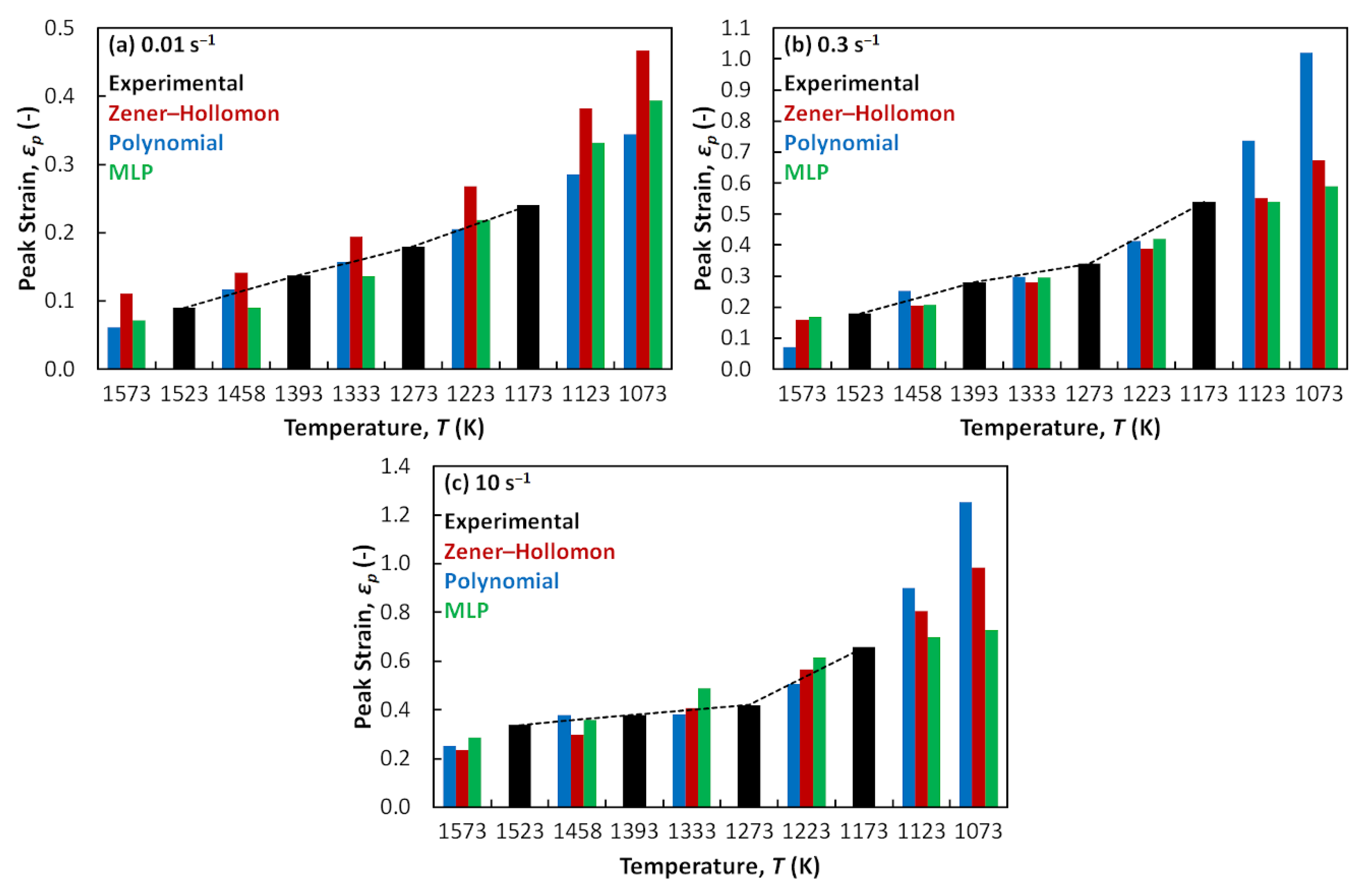
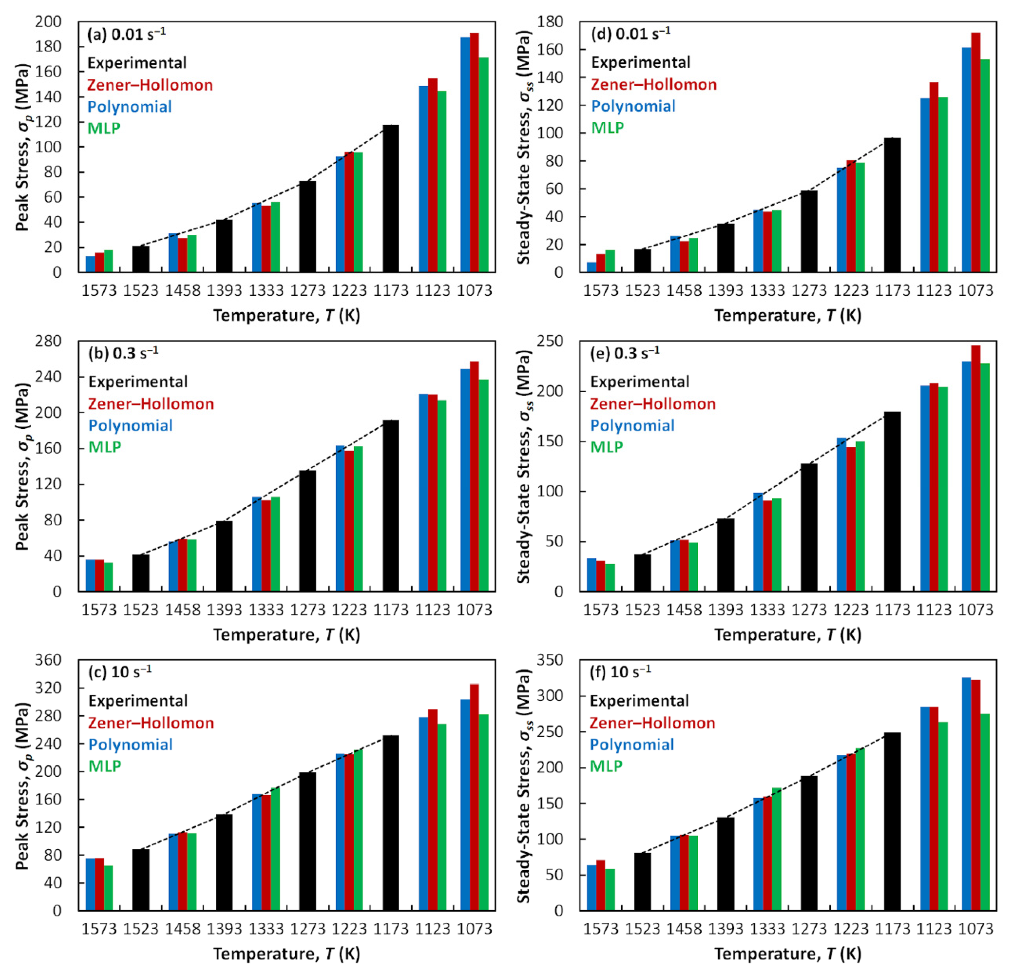
In order to compare the prediction possibilities of all applied approaches, Figure 6 and Figure 7 offer a prediction under non-experimentally tested conditions (inside and also outside of the tested temperature range). It is apparent that the biggest differences among the applied approaches have been obtained in the case of the εp-prediction. The ZH-based approach is evidently not suitable for the prediction under lower strain rates—Figure 6a. Predicted values (the red ones) are in this case overestimated—εp-values predicted under specific temperatures (e.g., 1573, 1458, 1333, and 1223 K) are illogically higher than those that were experimentally obtained under the nearest lower temperatures (the black ones). An opposite situation is then visible in the case of the 1458 K/10 s−1 (Figure 6c). In some cases (specifically at the 1573, 1458, 1333, and 1123 K under the 0.3 s−1) it seems that the predicted εp-values are also underestimated (almost the same level like in the case of the adjacent experimental εp-values). The MLP approach (green columns) then in the case of the εp-prediction struggles with similar issues like the ZH-based one—see e.g., overestimation under the 1333 K/10 s−1 or underestimated values at the 1458 and 1333 K under the 0.01 s−1.
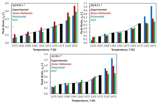
Figure 6.
Peak strain prediction inside and outside of the experimental conditions. (a) A strain rate of 0.01 s−1; (b) a strain rate of 0.3 s−1; and (c) a strain rate of 10 s−1. Black columns—experimental values; red columns—values predicted via the Zener–Hollomon approach; blue columns—values predicted via the multivariate polynomial approach; and green columns—values predicted via the multi-layer perceptron approach.
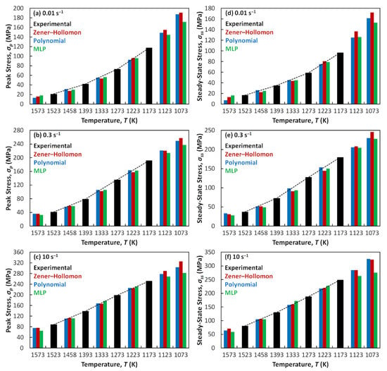
Figure 7.
Peak and steady-state stress prediction inside and outside of the experimental conditions. (a,d) A strain rate of 0.01 s−1; (b,e) a strain rate of 0.3 s−1; (c,f) a strain rate of 10 s−1. Black columns—experimental values; red columns—values predicted via the Zener–Hollomon approach; blue columns—values predicted via the multivariate polynomial approach; and green columns—values predicted via the multi-layer perceptron approach.
It seems that the polynomial approach (blue columns) offers in comparison with the previous ones much more reliable prediction—almost each predicted value perfectly fits into the experimentally given trend (see the black dashed lines). However, polynomial prediction gained under the 0.3 and 10 s−1 at lower temperatures (1123 and 1073 K) seems to be unduly overestimated—this can be caused by the purely polynomial character of the proposed approach, which can always bring a trend breach beyond the described data range. Nevertheless, despite of this issue, the polynomial approach is for the prediction purposes probably more suitable than the other ones—at least inside of the experimental data range. With respect to the σp and σss parameters, all approaches offer meaningful prediction—almost all predicted values of all approaches fit into the experimentally given trend (see the black dashed lines in Figure 7).
3.3. Evaluation of the Flow Curve Description
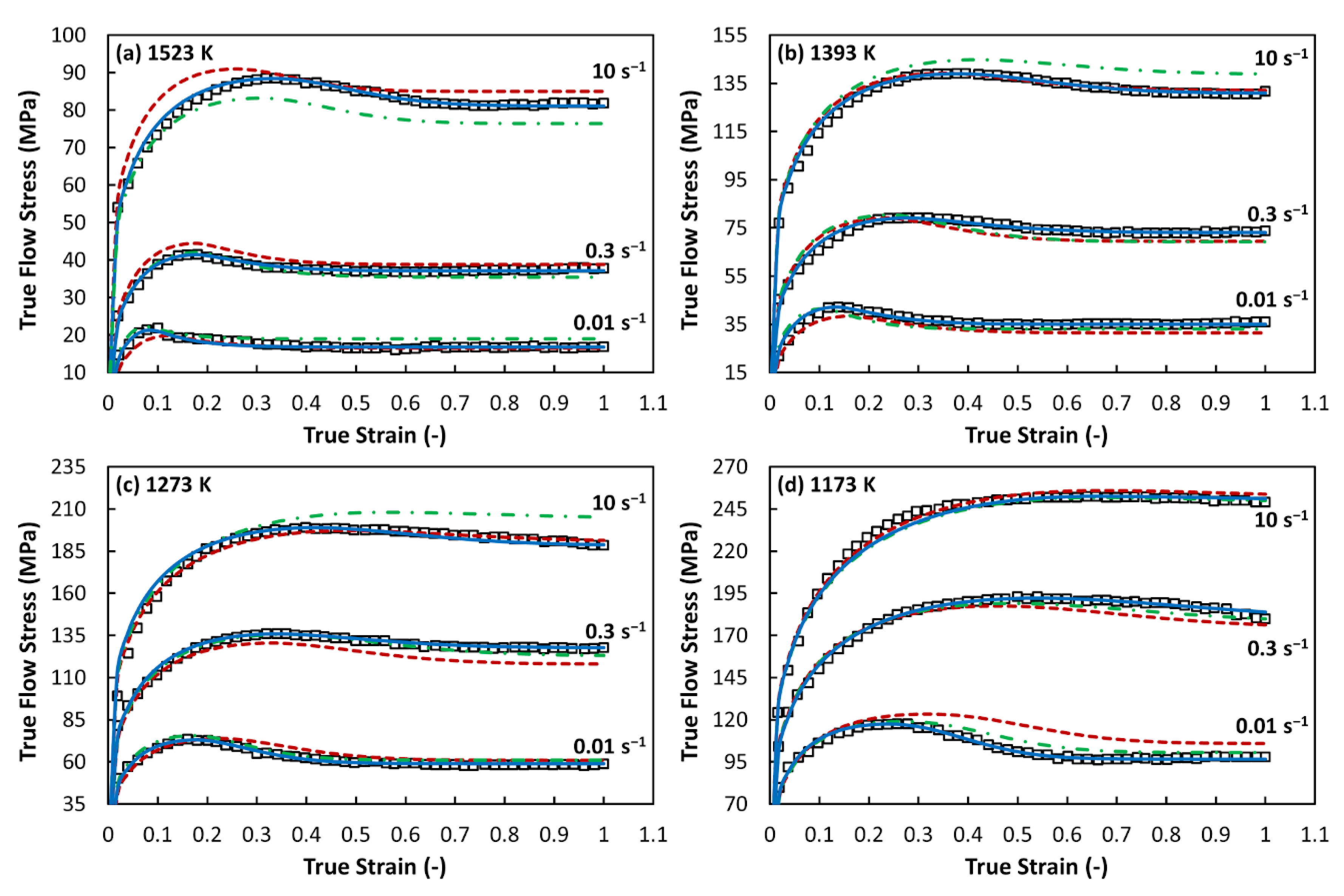
Table 6 displays the material constants for the description of the curve-shape-control parameters, i.e., c, n and k (Equation (2)). In addition, this table contains corresponding values of determination coefficient, R2 (-) [74] (Equation (12)). In this equation, with respect to the c, n, and k description, the Ti (-) and Ai (-) embody the values of the target (i.e., experimental) and approximated vectors of the specific parameter, respectively. The i = [1, n] ⊂ ℕ, where the n is the number of elements in these vectors (number of T- combinations, i.e., 12). The (-) then represents the mean values [75] of the target vectors. At a first glance it seems that the gained R2-values are not ideal—especially in the case of the n and k description. Nevertheless, the subsequent utilizing of the calculated parameters has showed that the shapes of the approximated flow curves are in accordance with the experimental ones—see the flow curve comparison in Figure 8.

Table 6.
Material constants for the description of c, n, and k parameters.
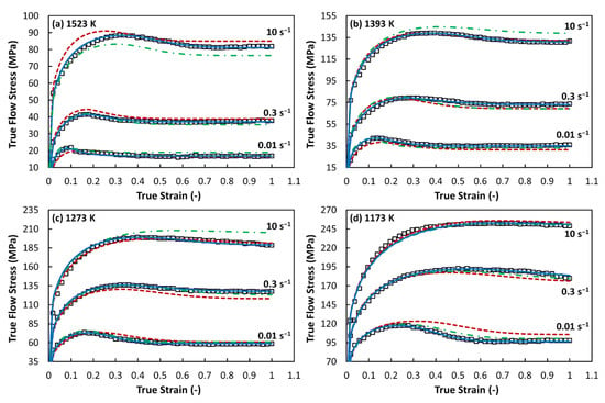
Figure 8.
Comparison between the experimental and via Equation (1) approximated flow curves. (a) A temperature of 1523 K; (b) a temperature of 1393 K; (c) a temperature of 1273 K; and (d) a temperature of 1173 K. Black boxes—experimental flow curves; red dash lines—approximated flow curves (peak and steady-state calculated via the Zener–Hollomon approach); blue solid lines—approximated flow curves (peak and steady-state calculated via the multivariate polynomial approach); and green dash-dot lines—approximated flow curves (peak and steady-state calculated via the multi-layer perceptron approach).
It is clear that a position of the calculated peak point coordinates plays a substantial role in accuracy of the flow curve description. This fact should be highly noticeable especially under higher deformation temperatures and lower strain rates—where the difference between the peak point and steady-state flow is usually more distinct (assumption of a more intensive course of softening processes, e.g., dynamic recrystallization). As demonstrated above, the best peak point and steady-state description has been obtained with the use of the multivariate polynomial approximation. As can be seen, Figure 8 practically confirms this result—the blue solid curves are almost identical with the experimental one. The calculated flow curves incorporating the coordinates approximated via other approaches offer in some cases distinctly lower accuracy—see namely the 1523 K, 1393 K, and 1273 K under the 10 s−1 and 1173 K/0.01 s−1. Although the shape of these curves is in accordance with the shape of the experimental ones, the inaccurately calculated peak and steady-state coordinates caused inconvenient shift out of the required position.
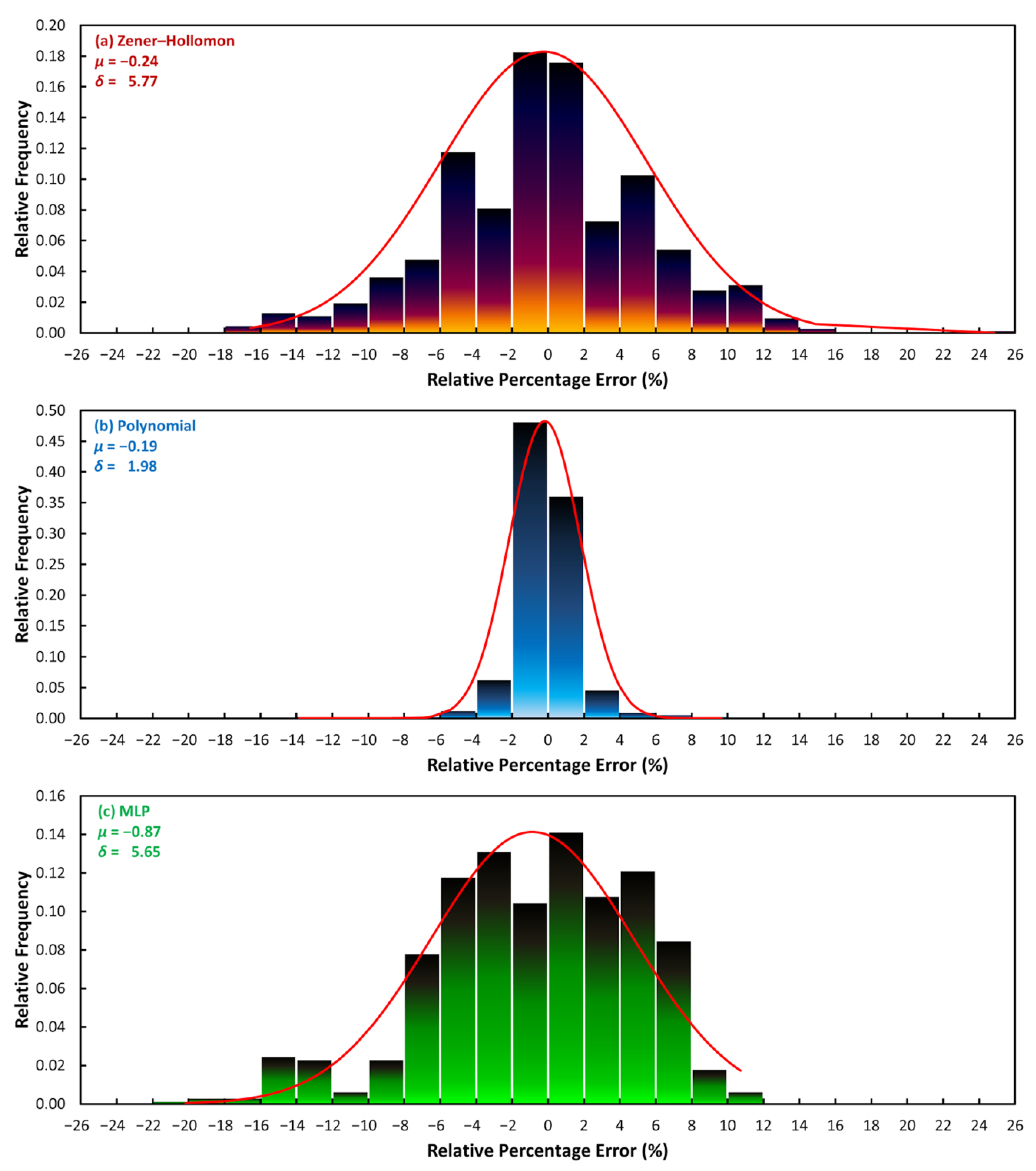
The statistical point of view on the discussed flow curve description is offered in Figure 9.
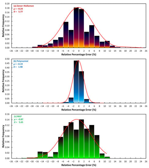
Figure 9.
Distribution of the relative percentage error achieved after the flow curve description via Equation (1). (a) Peak and steady-state calculated via the Zener–Hollomon approach; (b) peak and steady-state calculated via the multivariate polynomial approach; (c) peak and steady-state calculated via the multi-layer perceptron approach.
The assembled histograms capture the distribution of the relative percentage error, η (%) [76]:
The gained η-vectors have been subsequently evaluated via the mean value, μ (%) [75], and standard deviation, δ (%) [77]:
The Ti (MPa) and Ai (MPa) embody the values of the target (i.e., experimental) and approximated flow stress vectors, respectively. The i = [1, n] ⊂ ℕ, where the n is the number of elements in these vectors. It is apparent that the η-values associated with an application of the polynomial approach take narrower range (from −14% to 10%) in comparison with the ZH-based approach (from −18% to 26%) and MLP approach (from −22% to 12%). In addition, as regards to the polynomial approach, majority of the η-values (ca 84%) are ranging only between the −2% and 2%, which cannot be said about the others applied approaches. Neither the ZH-based approach nor the MLP approach achieves so favorable μ and δ values as the polynomial one. Moreover, the η-layout of the MLP approach does not correspond entirely with the normal (Gaussian [78]) distribution—which can be probably attributed to the neural-network nature of the performed calculations. So, the performed statistical evaluation clearly demonstrates predominance of the polynomial approach and practically confirms the conclusions of the above-performed flow curve comparison.
4. Conclusions
In the submitted research, the standardly used Zener–Hollomon (ZH) based equations, multi-layer perceptron (MLP) networks and multivariate polynomials have been evaluated with respect to the possibilities of the flow-curve characteristic coordinates (i.e., peak strain, peak and steady-state stress) description. The investigation has been realized on an experimentally gained flow curve dataset of an Invar 36 alloy acquired in a temperature range of 1173–1523 K, strain rate range of 0.01–10 s−1 and under true strain values reaching up to 1.0.
A statistical comparison between the target and approximated coordinates has showed that the highest approximation accuracy is provided by the multivariate polynomial approach. The ZH-based equations and the MLP networks were still able to offer a satisfactory approximation. However, both approaches and especially the MLP one show in the case of some coordinates excessively large errors.
Prediction ability of the applied approaches has been examined inside and also outside of the experimental dataset. Results of this evaluation have showed that both ZH-based and MLP approaches have a tendency either to overestimate or to underestimate the predicted peak strain coordinates. On the other hand, the prediction of the peak and steady-state stress values is appeared to be fine. The polynomial approach then provides a meaningful prediction for all studied coordinates.
The calculated coordinates have been subsequently inserted into the flow stress models to describe the experimentally achieved flow curves in their whole strain range. As expected, by-the-polynomial-approach calculated coordinates have a positive influence on the accuracy of the utilized flow stress models. On the other hand, incorporation of the ZH and MLP coordinates leads to the displacement of the calculated flow curves beyond the experimental data.
Based on the obtained results, it can be stated that the approximation accuracy and prediction possibilities of the multivariate-polynomial approach are higher in comparison to the ZH-based and MLP ones. Despite of this fact, the approximation accuracy of both ZH and MLP approaches can be still considered as sufficient. Either way, neither the ZH approach nor the MLP approach can be in this case recommended for the practical usage—they encounter on the obstacles when trying to predict the peak strain coordinates outside and also inside of the experimental conditions.
Author Contributions
Conceptualization, Methodology, Software, Supervision, Visualization and Writing—original draft, P.O.; Data curation, P.O. and P.K.; Formal analysis, P.O. and S.R.; Investigation, P.O. and H.N.; Project administration and Resources, I.S.; Validation, P.O., P.K., I.S., R.K., and S.R.; Writing—review and editing, P.O., P.K., R.K., and H.N. All authors have read and agreed to the published version of the manuscript.
Funding
This research was funded by the project no. CZ.02.1.01/0.0/0.0/17_049/0008399 from the EU and CR financial funds provided by the Operational Programme “Research, Development and Education” and in within the frame of the Student Grant Competition SP2020/88 funded by Ministry of Education, Youth and Sports of the Czech Republic.
Conflicts of Interest
The authors declare no conflict of interest. The funders had no role in the design of the study; in the collection, analyses, or interpretation of data; in the writing of the manuscript, or in the decision to publish the results.
References
- Gronostajski, Z. The Constitutive Equations for FEM Analysis. J. Mater. Process. Technol. 2000, 106, 40–44. [Google Scholar] [CrossRef]
- Ebrahimi, R.; Shafiei, E. Mathematical Modeling of Single Peak Dynamic Recrystallization Flow Stress Curves in Metallic Alloys. In Recrystallization; Sztwiertnia, K., Ed.; InTech: Rijeka, Croatia, 2012; pp. 207–225. [Google Scholar] [CrossRef]
- Fields, D.S.; Backofen, W.A. Determination of Strain Hardening Characteristics by Torsion Testing. Proc. ASTM 1957, 57, 1259–1272. [Google Scholar]
- Johnson, G.R.; Cook, W.H. A Constitutive Model and Data for Metals Subjected to Large Strains, High Strain Rates and High Temperatures. In Proceedings of the 7th International Symposium on Ballistics, The Hague, The Netherlands, 19–21 April 1983; American Defense Preparedness Association: Arlington, VA, USA, 1983; pp. 541–547. [Google Scholar]
- Cingara, A.; McQueen, H.J. New Formula for Calculating Flow Curves from High Temperature Constitutive Data for 300 Austenitic Steels. J. Mater. Process. Technol. 1992, 36, 31–42. [Google Scholar] [CrossRef]
- Ebrahimi, R.; Zahiri, S.H.; Najafizadeh, A. Mathematical Modelling of the Stress–Strain Curves of Ti-IF Steel at High Temperature. J. Mater. Process. Technol. 2006, 171, 301–305. [Google Scholar] [CrossRef]
- Lin, Y.C.; Chen, M.-S.; Zhong, J. Constitutive Modeling for Elevated Temperature Flow Behavior of 42CrMo Steel. Comput. Mater. Sci. 2008, 42, 470–477. [Google Scholar] [CrossRef]
- Mandal, S.; Rakesh, V.; Sivaprasad, P.V.; Venugopal, S.; Kasiviswanathan, K.V. Constitutive Equations to Predict High Temperature Flow Stress in a Ti-Modified Austenitic Stainless Steel. Mater. Sci. Eng. A 2009, 500, 114–121. [Google Scholar] [CrossRef]
- Momeni, A.; Dehghani, K.; Ebrahimi, G.R.; Keshmiri, H. Modeling the Flow Curve Characteristics of 410 Martensitic Stainless Steel under Hot Working Condition. Metall. Mater. Trans. A 2010, 41, 2898–2904. [Google Scholar] [CrossRef]
- Mirzadeh, H.; Najafizadeh, A. Flow Stress Prediction at Hot Working Conditions. Mater. Sci. Eng. A 2010, 527, 1160–1164. [Google Scholar] [CrossRef]
- Mirzadeh, H.; Najafizadeh, A. Extrapolation of Flow Curves at Hot Working Conditions. Mater. Sci. Eng. A 2010, 527, 1856–1860. [Google Scholar] [CrossRef]
- Shafaat, M.A.; Omidvar, H.; Fallah, B. Prediction of Hot Compression Flow Curves of Ti–6Al–4V Alloy in α + β Phase Region. Mater. Des. 2011, 32, 4689–4695. [Google Scholar] [CrossRef]
- YU, B.-J.; Guan, X.-J.; Wang, L.-J.; Zhao, J.; Liu, Q.-Q.; Cao, Y. Hot Deformation Behavior and Constitutive Relationship of Q420qE Steel. J. Cent. South Univ. Technol. 2011, 18, 36–41. [Google Scholar] [CrossRef]
- Lin, Y.C.; Li, Q.-F.; Xia, Y.-C.; Li, L.-T. A Phenomenological Constitutive Model for High Temperature Flow Stress Prediction of Al–Cu–Mg Alloy. Mater. Sci. Eng. A 2012, 534, 654–662. [Google Scholar] [CrossRef]
- Fereshteh-Saniee, F.; Barati, F.; Badnava, H.; Nejad, K.F. An Exponential Material Model for Prediction of the Flow Curves of Several AZ Series Magnesium Alloys in Tension and Compression. Mater. Des. 2012, 35, 1–11. [Google Scholar] [CrossRef]
- Changizian, P.; Zarei-Hanzaki, A.; Roostaei, A.A. The High Temperature Flow Behavior Modeling of AZ81 Magnesium Alloy Considering Strain Effects. Mater. Des. 2012, 39, 384–389. [Google Scholar] [CrossRef]
- Li, H.-Y.; Wei, D.-D.; Hu, J.-D.; Li, Y.-H.; Chen, S.-L. Constitutive Modeling for Hot Deformation Behavior of T24 Ferritic Steel. Comput. Mater. Sci. 2012, 53, 425–430. [Google Scholar] [CrossRef]
- Nayak, K.C.; Date, P.P. Development of Constitutive Relationship for Thermomechanical Processing of Al-SiC Composite Eliminating Deformation Heating. J. Mater. Eng. Perform. 2019, 28, 5323–5343. [Google Scholar] [CrossRef]
- Sheikhali, A.H.; Morakkabati, M.; Abbasi, S.M. Constitutive Modeling for Hot Working Behavior of SP-700 Titanium Alloy. J. Mater. Eng. Perform. 2019, 28, 6525–6537. [Google Scholar] [CrossRef]
- Schindler, I.; Kawulok, P.; Očenášek, V.; Opěla, P.; Kawulok, R.; Rusz, S. Flow Stress and Hot Deformation Activation Energy of 6082 Aluminium Alloy Influenced by Initial Structural State. Metals 2019, 9, 1248. [Google Scholar] [CrossRef]
- Hensel, A.; Spittel, T. Kraft- und Arbeitsbedarf bildsamer Formgebungsverfahren, 1st ed.; Deutscher Verlag für Grundstoffindustrie: Leipzig, Germany, 1978. [Google Scholar]
- Solhjoo, S. Analysis of Flow Stress up to the Peak at Hot Deformation. Mater. Des. 2009, 30, 3036–3040. [Google Scholar] [CrossRef]
- Solhjoo, S. Determination of Critical Strain for Initiation of Dynamic Recrystallization. Mater. Des. 2010, 31, 1360–1364. [Google Scholar] [CrossRef]
- Solhjoo, S. Determination of Flow Stress under Hot Deformation Conditions. Mater. Sci. Eng. A 2012, 552, 566–568. [Google Scholar] [CrossRef]
- Solhjoo, S. Determination of Flow Stress and the Critical Strain for the Onset of Dynamic Recrystallization Using a Hyperbolic Tangent Function. Mater. Des. 2014, 54, 390–393. [Google Scholar] [CrossRef]
- Solhjoo, S. Determination of Flow Stress and the Critical Strain for the Onset of Dynamic Recrystallization Using a Sine Function. Available online: https://arxiv.org/ftp/arxiv/papers/1405/1405.0196.pdf (accessed on 19 May 2020).
- Solhjoo, S.; Vakis, A.I.; Pei, Y.T. Two Phenomenological Models to Predict the Single Peak Flow Stress Curves up to the Peak during Hot Deformation. Mech. Mater. 2017, 105, 61–66. [Google Scholar] [CrossRef]
- Spigarelli, S.; El Mehtedi, M. A New Constitutive Model for the Plastic Flow of Metals at Elevated Temperatures. J. Mater. Eng. Perform. 2014, 23, 658–665. [Google Scholar] [CrossRef]
- Quan, G.; Tong, Y.; Luo, G.; Zhou, J. A Characterization for the Flow Behavior of 42CrMo Steel. Comput. Mater. Sci. 2010, 50, 167–171. [Google Scholar] [CrossRef]
- Shen, J.; Hu, L.; Sun, Y.; Wan, Z.; Feng, X.; Ning, Y. A Comparative Study on Artificial Neural Network, Phenomenological-Based Constitutive and Modified Fields–Backofen Models to Predict Flow Stress in Ti-4Al-3V-2Mo-2Fe Alloy. J. Mater. Eng. Perform. 2019, 28, 4302–4315. [Google Scholar] [CrossRef]
- Akbari, Z.; Mirzadeh, H.; Cabrera, J.-M. A Simple Constitutive Model for Predicting Flow Stress of Medium Carbon Microalloyed Steel during Hot Deformation. Mater. Des. 2015, 77, 126–131. [Google Scholar] [CrossRef]
- Mohamadizadeh, A.; Zarei-Hanzaki, A.; Abedi, H.R. Modified Constitutive Analysis and Activation Energy Evolution of a Low-Density Steel Considering the Effects of Deformation Parameters. Mech. Mater. 2016, 95, 60–70. [Google Scholar] [CrossRef]
- Liu, L.; Wu, Y.-X.; Gong, H.; Wang, K. Modification of Constitutive Model and Evolution of Activation Energy on 2219 Aluminum Alloy during Warm Deformation Process. Trans. Nonferrous Met. Soc. China 2019, 29, 448–459. [Google Scholar] [CrossRef]
- Wang, F.; Shen, J.; Zhang, Y.; Ning, Y. A Modified Constitutive Model for the Description of the Flow Behavior of the Ti-10V-2Fe-3Al Alloy during Hot Plastic Deformation. Metals 2019, 9, 844. [Google Scholar] [CrossRef]
- Anand, L. Constitutive Equations for the Rate-Dependent Deformation of Metals at Elevated Temperatures. J. Eng. Mater. Technol. 1982, 104, 12–17. [Google Scholar] [CrossRef]
- Koric, S.; Thomas, B.G. Thermo-Mechanical Models of Steel Solidification Based on Two Elastic Visco-Plastic Constitutive Laws. J. Mater. Process. Technol. 2008, 197, 408–418. [Google Scholar] [CrossRef]
- Kozlowski, P.F.; Thomas, B.G.; Azzi, J.A.; Wang, H. Simple Constitutive Equations for Steel at High Temperature. Metall. Mater. Trans. A 1992, 23, 903–918. [Google Scholar] [CrossRef]
- Quan, G.-Z.; Zou, Z.-Y.; Wang, T.; Liu, B.; Li, J.-C. Modeling the Hot Deformation Behaviors of As-Extruded 7075 Aluminum Alloy by an Artificial Neural Network with Back-Propagation Algorithm. High. Temp. Mater. Process. 2017, 36, 1–13. [Google Scholar] [CrossRef]
- Lv, J.; Ren, H.; Gao, K. Artificial Neural Network-Based Constitutive Relationship of Inconel 718 Superalloy Construction and its Application in Accuracy Improvement of Numerical Simulation. Appl. Sci. 2017, 7, 124. [Google Scholar] [CrossRef]
- Yan, J.; Pan, Q.L.; Li, A.D.; Song, W.B. Flow Behavior of Al-6.2Zn-0.70Mg-0.30Mn-0.17Zr Alloy During Hot Compressive Deformation Based on Arrhenius and ANN Models. Trans. Nonferrous Met. Soc. China 2017, 27, 638–647. [Google Scholar] [CrossRef]
- Lin, Y.C.; Liang, Y.J.; Chen, M.S.; Chen, X.M. A Comparative Study on Phenomenon and Deep Belief Network Models for Hot Deformation Behavior of an Al–Zn–Mg–Cu Alloy. Appl. Phys. A Mater. Sci. Process. 2017, 123, 68. [Google Scholar] [CrossRef]
- Opěla, P.; Kawulok, P.; Kawulok, R.; Kotásek, O.; Buček, P.; Ondrejkovič, K. Extension of Experimentally Assembled Processing Maps of 10CrMo9-10 Steel via a Predicted Dataset and the Influence on Overall Informative Possibilities. Metals 2019, 9, 1218. [Google Scholar] [CrossRef]
- Song, S.H. A Comparison Study of Constitutive Equation, Neural Networks, and Support Vector Regression for Modeling Hot Deformation of 316L Stainless Steel. Materials 2020, 13, 3766. [Google Scholar] [CrossRef]
- Mozaffar, M.; Bostanabad, R.; Chen, W.; Ehmann, K.; Cao, J.; Bessa, M.A. Deep learning predicts path-dependent plasticity. Proc. Natl. Acad. Sci. USA 2019, 116, 26414–26420. [Google Scholar] [CrossRef]
- Abueidda, D.W.; Koric, S.; Sobh, N.A.; Sehitoglu, H. Deep learning for plasticity and thermo-viscoplasticity. Int. J. Plast. 2020, 136, 102852. [Google Scholar] [CrossRef]
- Wu, S.W.; Zhou, X.G.; Cao, G.M.; Liu, Z.Y.; Wang, G.D. The Improvement on Constitutive Modeling of Nb-Ti Micro Alloyed Steel by Using Intelligent Algorithms. Mater. Des. 2017, 116, 676–685. [Google Scholar] [CrossRef]
- Opěla, P.; Schindler, I.; Kawulok, P.; Kawulok, R.; Rusz, S.; Rodak, K. Hot Flow Curve Description of CuFe2 Alloy via Different Artificial Neural Network Approaches. J. Mater. Eng. Perform. 2019, 28, 4863–4870. [Google Scholar] [CrossRef]
- Pietrzyk, M.; Kusiak, J.; Szeliga, D.; Rauch, Ł.; Sztangret, Ł.; Górecki, G. Application of Metamodels to Identification of Metallic Materials Models. Adv. Mater. Sci. Eng. 2016, 2016, 2357534. [Google Scholar] [CrossRef][Green Version]
- Sztangret, Ł.; Szeliga, D.; Kusiak, J.; Pietrzyk, M. Application of Inverse Analysis with Metamodelling for Identification of Metal Flow Stress. Can. Metall. Q. 2012, 51, 440–446. [Google Scholar] [CrossRef]
- Zener, C.; Hollomon, J.H. Effect of Strain Rate upon Plastic Flow of Steel. J. Appl. Phys. 1944, 15, 22–32. [Google Scholar] [CrossRef]
- Schindler, I.; Kawulok, P.; Kawulok, R.; Hadasik, E.; Kuc, D. Influence of Calculation Method on Value of Activation Energy in Hot Forming. High Temp. Mater. Processes 2013, 32, 149–155. [Google Scholar] [CrossRef]
- Razali, M.K.; Irani, M.; Joun, M.S. General Modeling of Flow Stress Curves of Alloys at Elevated Temperatures Using Bi-Linearly Interpolated or Closed-Form Functions for Material Parameters. J. Mater. Res. Technol. 2019, 8, 2710–2720. [Google Scholar] [CrossRef]
- GLEEBLE: Gleeble®Thermal-Mechanical Simulators. Available online: https://gleeble.com/ (accessed on 1 October 2019).
- Kolmogorov, A.N. К статистическoй теoрии кристаллизации металлoв [On the statistics of crystallization processes in metals]. Izvestiya Akademii Nauk SSSR. Seriya Matematicheskaya 1937, 1, 355–359. [Google Scholar]
- Wei, H.-L.; Liu, G.-Q.; Xiao, X.; Zhang, M.-H. Dynamic Recrystallization Behavior of a Medium Carbon Vanadium Microalloyed Steel. Mater. Sci. Eng. A 2013, 573, 215–221. [Google Scholar] [CrossRef]
- Legendre, A.M. Nouvelles méthodes pour la détermination des orbites des comètes [New Methods for the Determination of the Orbits of Comets]; Firmin-Didot: Mesnil-sur-I’Estrée, France, 1805. [Google Scholar]
- Opěla, P.; Schindler, I.; Kawulok, P.; Vančura, F.; Kawulok, R.; Rusz, S. New Model Predicting Flow Curves in Wide Range of Thermomechanical Conditions of 38MnVS6 Steel. In Proceedings of the Metal 2016: 25th Anniversary International Conference on Metallurgy and Materials, Brno, Czech Republic, 25–27 May 2016; Tanger Ltd.: Ostrava, Czech Republic, 2017; pp. 458–463. [Google Scholar]
- Levenberg, K. A Method for the Solution of Certain Non-Linear Problems in Least Squares. Quart. Appl. Math. 1944, 2, 164–168. [Google Scholar] [CrossRef]
- Marquardt, D.W. An Algorithm for Least-Squares Estimation of Nonlinear Parameters. J. Soc. Indust. Appl. Math. 1963, 11, 431–441. [Google Scholar] [CrossRef]
- Roweis, S. Levenberg-Marquardt Optimization. Available online: https://cs.nyu.edu/~roweis/notes/lm.pdf (accessed on 1 October 2019).
- Garofalo, F. An Empirical Relation Defining the Stress Dependence of Minimum Creep Rate in Metals. Trans. Metall. Soc-AIME 1963, 227, 351–356. [Google Scholar]
- McCulloch, W.S.; Pitts, W.H. A Logical Calculus of Ideas Immanent in Nervous Activity. Bull. Math. Biophys. 1943, 5, 115–133. [Google Scholar] [CrossRef]
- Rosenblatt, F. The Perceptron: A Probabilistic Model for Information Storage and Organization in the Brain. Psychological Review 1958, 65, 386–408. [Google Scholar] [CrossRef] [PubMed]
- Krenker, A.; Bešter, J.; Kos, A. Introduction to the Artificial Neural Networks. In Artificial Neural Networks—Methodological Advances and Biomedical Applications; Suzuki, K., Ed.; InTech: Rijeka, Croatia, 2011; pp. 3–18. [Google Scholar]
- Gauss, J.C.F. Theoria Combinationis Observationum Erroribus Minimis Obnoxiae [Theory of the Combination of Observations Least Subject to Errors]; Henricum Dieterich: Göttingen, Germany, 1823; pp. 53–57. [Google Scholar]
- Bayes, T.; Price, R. An Essay towards solving a Problem in the Doctrine of Chance. By the late Rev. Mr. Bayes, F.R.S. communicated by Mr. Price, in a letter to John Canton, A.M.F.R.S. Phil. Trans. 1763, 53, 370–418. [Google Scholar] [CrossRef]
- MacKey, D.J.C. Bayesian interpolation. Neural Comput. 1992, 4, 415–447. [Google Scholar] [CrossRef]
- Rumelhart, D.E.; Hinton, G.E.; Williams, R.J. Learning Internal Representations by Error Propagation. In Parallel Distributed Processing: Explorations in the Microstructure of Cognition; Feldman, J.A., Hayes, P.J., Rumelhart, D.E., Eds.; The MIT Press: Cambridge, USA, 1986; Volume 1: Foundations, pp. 318–362. [Google Scholar]
- Debes, K.; Koenig, A.; Gross, H.M. Transfer Functions in Artificial Neural Networks: A Simulation-Based Tutorial. Available online: https://www.brains-minds-media.org/archive/151/ (accessed on 16 September 2019).
- MathWorks. MATLAB® Math. Graphics. Programming. Available online: https://www.mathworks.com/products/matlab.html (accessed on 18 September 2019).
- Beale, M.H.; Hagan, M.T.; Demuth, H.B. Neural Network ToolboxTM 7: User’s Guide. Available online: https://www2.cs.siu.edu/~rahimi/cs437/slides/nnet.pdf (accessed on 18 September 2019).
- Descartes, R. Discours de la méthode pour bien conduire sa raison, & chercher la vérité dans les sciences. Plus la dioptrique. Les météores. Et la géométrie. [Discourse on the Method of Rightly Conducting One’s Reason and of Seeking Truth in the Sciences. Plus the Diopter, Meteors and Geometry]; De l’imprimerie de Ian Maire: Leiden, The Netherlands, 1637. [Google Scholar]
- Gnuplot: Portable Command-Line Driven Graphing Utility. Available online: http://www.gnuplot.info/ (accessed on 18 September 2019).
- Wright, S. Correlation and Causation. J. Agric. Res. 1921, 20, 557–585. [Google Scholar]
- Simpson, T. A letter to the Right Honourable George Earl of Macclesfield, President of the Royal Society, On the Advantage of Taking the Mean of a Number of Observations in Practical Astronomy. Philos. Trans. 1755, 49, 82–93. [Google Scholar] [CrossRef][Green Version]
- Abramowitz, M.; Stegun, I.A. Handbook of Mathematical Functions with Formulas, Graphs, and Mathematical Tables, 9th ed.; Dover Publications: Mineola, NY, USA, 1972; p. 14. [Google Scholar]
- Pearson, K. On the dissection of asymmetrical frequency curves. Phil. Trans. Roy. Soc. Lond. Ser. A 1894, 185, 719–810. [Google Scholar]
- Gauss, J.C.F. Theoria motus corporum coelestium in sectionibus conicis solem ambientium [Theory of the Motion of the Heavenly Bodies Moving about the Sun in Conic Sections]; Friedrich Perthes and I. H. Besser: Hamburg, Germany, 1809. [Google Scholar]
Publisher’s Note: MDPI stays neutral with regard to jurisdictional claims in published maps and institutional affiliations. |
© 2020 by the authors. Licensee MDPI, Basel, Switzerland. This article is an open access article distributed under the terms and conditions of the Creative Commons Attribution (CC BY) license (http://creativecommons.org/licenses/by/4.0/).

