FE Analysis of Laser Shock Peening on STS304 and the Effect of Static Damping on the Solution

Abstract

Laser shock peening creates compressive residual stress on the surface of the material, reducing stress corrosion cracking and increasing fatigue life. FE simulation of laser shock peening is an effective way to determine the mechanical effects on the material. In conventional FE simulations of laser shock peening, explicit analysis is used while pressure loads are applied and switched into implicit analysis to dissipate kinetic energy. In this study, static damping was adopted to dissipate kinetic energy without conversion into implicit analysis. Simulation of a single laser shock and multiple shocks was performed, and deformation and minimum principal stress were compared to evaluate the static damping effect. The history of the internal and kinetic energy were analyzed to compare the stabilization time depending on the damping value. Laser shock peening experiments were also performed on stainless steel 304 material. The residual stress of the specimen was measured by the hole drilling method and it was compared to the FE simulation result. The residual stress from the experiment and the simulation results showed similar distributions in the depth direction. Anisotropic residual stress distribution due to the laser path was observed in both results.

1. Introduction

The peening process generates a compressive residual stress field on the surface of a material. Shot peening and ultrasonic peening not only largely deform the material surface but also generate the compressive residual stresses within a few micrometers of depth. On the other hand, laser shock peening (LSP) is known to improve the fatigue life by 4 to 5 times compared to other peening processes by forming compressive residual stress at the depth of several millimeters from the material surface. The LSP generates compressive residual stress by a plasma shock induced by the reaction between a high-energy laser pulse and the material [1]. When the plasma pressure is applied on the material surface, it deforms plastically and pushes near the material. As an interaction, the elastic region pushes back to the plastically deformed zone, and the compressive residual stress remains as a result. The compressive residual stress and the grain refinement generated by laser shock peening are known to increase the stress corrosion cracking resistance and fatigue life of the alloy [2,3]. However, the LSP process is mainly applied to high-added-value products because of the high process cost compared to other peening processes [4]. For example, mechanical parts subjected to fatigue loads, such as turbine blades, or subjected to corrosive environments, such as welded parts in nuclear reactors, are the main applications for LSP [5].

Since FEM analysis of the LSP was firstly introduced by Braisted and Brockman [6] in 1999, several studies have been reported based on ABAQUS [7,8,9,10,11,12] and ANSYS LS-DYNA [13,14,15]. The LSP process is usually performed within an instant. Plasma pressure loading takes less than 200 ns and the material plastically deforms. Due to this process characteristic, FE simulation of the LSP is analyzed by explicit methods. The explicit analysis is considered in the case of a non-linear problem, but it requires a much longer calculation time than implicit analysis due to the small time step size. During the pressure loading period, the FE model is solved by an explicit method. To de-excite the model after pressure loading, the explicit analysis result is exported to implicit analysis and it repeats until final loading, as shown in Figure 1 [16]. Peyre et al. [8] performed LSP FE simulation of 12% Cr stainless steel based on the strain-rate-dependent stress–strain relationship of the Johnson and Cook model. Two-step analysis was repeated, where the first step was loading and the second was calculating the deformation and residual stress field. However, the procedure needed 1 ms for stabilization; as a result, it took one hour (wall-clock) per shot. Amarchinta et al. [9] performed LSP FE simulation of Ti–6Al–4V material by using the Johnson–Cook and Zerilli–Armstrong stress–strain models. Depending on the laser pulse energy, residual stress was evaluated according to depth. As a simulation method, the pressure loads were applied through explicit analysis and residual stress was analyzed by implicit analysis. As shown in Figure 1, Hasser et al. [17] proposed SEATD analysis, which does not need to switch into implicit analysis but applies time-dependent damping after the loading period to stabilize the model. This method was performed six-times faster in terms of the total calculation time than the 2N + 1 analysis method that was proposed by Brockman et al. [18]. Bahmare et al. [15] performed LS-DYNA-based LSP simulation with the Zerilli and Armstrong model for Ti–6Al–2Sn–4Zr–2Mo material. Only explicit analysis with damping was used for stabilization, but the damping value was not described in detail. Fameso et al. [19] used explicit analysis only and they employed time-stepped damping during the loading step and viscous damping during the no-loading step. Residual stress derived from the simulation and experiment showed a close correlation in terms of distribution, and total CPU time was reduced to one third compared to conventional explicit–implicit methods.

Compared to the LS-DYNA, the Autodyn requires the optional license to transfer the explicit analysis result to an implicit solver. In this work, to settle the model without converting the analysis from explicit to implicit, static damping is employed. Similar to Fameso et al.’s study [19], the static damping was applied during both the loading and relaxation period. The effect of the static damping on the FE simulation was evaluated from the single LSP and overlapped multiple LSP simulation results. Comparison of the residual stress of the LSP-treated material and LSP simulation was discussed.

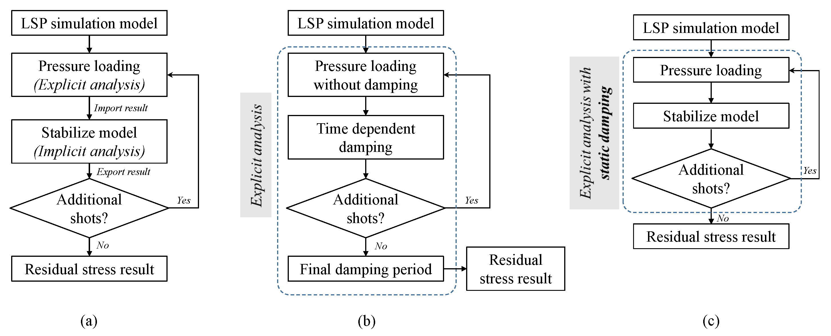
2. LSP Process Modeling

2.1. Conservation Equations for Explicit Analysis

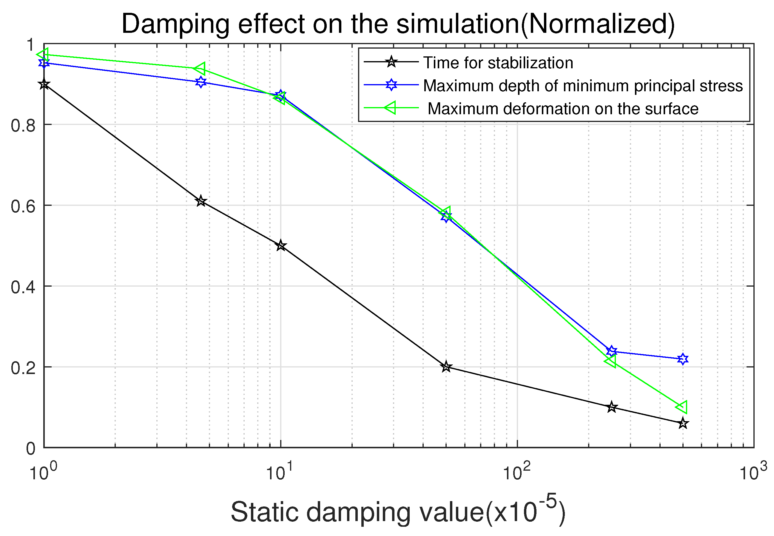
The partial difference equations (PDE) expressed as mass, momentum and energy conservation need to be solved in explicit analysis. The FE model, boundary condition, initial condition and loading condition are also calculated. Each conservation equation can be expressed as [20] follows. The $\rho$ is density; V is volume; m is mass; $\ddot{x}$, $\ddot{y}$ and $\ddot{z}$ are the x, y and z direction acceleration; b is the momentum term; ${\sigma }_{ij}$ is the stress tensor; $\dot{e}$ is the energy rate; and ${\dot{\epsilon }}_{ij}$ is the strain rate tensor.

Mass conservation equation:

$$\frac{{\rho }_0{V}_0}{V}=\frac{m}{V}$$

(1)

Momentum conservation equation:

$$\begin{array}{c}\hfill \rho \ddot{x}=b_x+\frac{\delta {\sigma }_{xx}}{{\delta }_x}+\frac{\delta {\sigma }_{xy}}{{\delta }_y}+\frac{\delta {\sigma }_{xz}}{{\delta }_z}\\ \hfill \rho \ddot{y}=b_y+\frac{\delta {\sigma }_{yx}}{{\delta }_x}+\frac{\delta {\sigma }_{yy}}{{\delta }_y}+\frac{\delta {\sigma }_{yz}}{{\delta }_z}\\ \hfill \rho \ddot{z}=b_z+\frac{\delta {\sigma }_{zx}}{{\delta }_x}+\frac{\delta {\sigma }_{zy}}{{\delta }_y}+\frac{\delta {\sigma }_{zz}}{{\delta }_z}\end{array}$$

(2)

Energy conservation equation:

$$\dot{e}=\frac{1}{\rho }({\sigma }_{xx}{\dot{\epsilon }}_{xx}+{\sigma }_{yy}{\dot{\epsilon }}_{yy}+{\sigma }_{zz}{\dot{\epsilon }}_{zz}+2{\sigma }_{xy}{\dot{\epsilon }}_{xy}+2{\sigma }_{yz}{\dot{\epsilon }}_{yz}+2{\sigma }_{zx}{\dot{\epsilon }}_{zx})$$

(3)

2.2. Static Damping

The ANSYS Autodyn solver was used to perform transient analysis and it presents a guideline for a proper static damping value [21,22]. The procedure introduces a damping force that is proportional to the nodal speed and aims to critically damp the lowest vibration mode of a static system. When the damping option is used, the nodal velocity is calculated every iteration in the solver as Equation (4):

$$v^{n+1/2}=(1-2\pi R_d)v^{n-1/2}+(1-\pi R_d)\dot{v}\Delta t^n$$

(4)

where v is the nodal velocity, $R_d$ is a static damping value, n is the time of the current iteration of the solver and $\Delta t$ is a time step during the solving process.

$$R_d=\frac{2\Delta t/T}{1+2\pi \Delta t/T}$$

(5)

Here, T is a period of the lowest mode of vibration. The values of $\Delta$t and T can be obtained by after first solving the FE model without the damping option. These values should be estimated by the user and the T should not be underestimated. The values that were used in this study will be discussed later.

2.3. Stress–Strain Model

Every material has its own stress–strain curve. These curves are mostly obtained by tensile tests. However, the LSP process deforms the material surface in a short time, and, in the case of a high strain rate (strain per time) process, the stress–strain curves change depending on the strain rate. There are several models of the high strain rate stress–strain relationship that are well known, such as as Johnson–Cook (JC) [23], Zerilli–Armstrong (ZA) [24] and the Khan–Huang–Liang (KHL) [25] equation.

The equation (6) is the JC model, where A, B, C, n and m are the material-dependent coefficients that are determined by the experiment. A is the yield strength; B is the hardening modulus; C is the strain rate dependency coefficient; $\epsilon$ is the effective plastic strain; $\dot{\epsilon }$ is the effective plastic strain rate; $\dot{{\epsilon }_0}$ is the reference strain rate; n is the work hardening exponential; m is the term of thermal softening [26]. The thermal term of the JC model is neglected because the LSP is regarding a non-thermal process [11,14,27]. The JC model was used in this study for FE simulation.

$$\sigma =[A+B{\left(\epsilon \right)}^n][1+Cln\left(\frac{\dot{\epsilon }}{\dot{{\epsilon }_0}}\right)][1-T^m]$$

(6)

2.4. Pressure Load Model

Several pressure loading models have been proposed in previous studies. The pressure load is expressed as a function of time, a simple triangular load model [13] and a step load model [14]. The pressure load profile applied in this work is shown in Figure 2. This normalized pressure load model was proposed in several studies [9,28].

The peak pressure can be calculated from Equation (7). Here, $P_{peak}\left(GPa\right)$ is the peak plasma pressure; $\alpha$ is the correction factor of the internal energy and the thermal energy (usually $\alpha \approx 0.25$ ); I ($\mathrm{GW}·{\mathrm{cm}}^{-2}$) is the laser pulse power density, where $P_{pulse}$ is the laser pulse power and $A_{peen}$ is the laser spot area at the working point; Z$(\mathrm{g}·{\mathrm{cm}}^{-2}{\mathrm{s}}^{-1})$ is the combined acoustic impedance of the confinement layer $Z_{water}(\approx 0.15\times {10}^6)$ of water and the target material $Z_{target}(\approx 4.5\times {10}^6)$ of stainless steel [8,12,29,30].

$$P_{peak}=0.01\sqrt{\frac{\alpha }{2\alpha +3}·Z·I}$$

(7)

$$\begin{array}{cc}\hfill \frac{2}{Z}=& \frac{1}{Z_{water}}+\frac{1}{Z_{taget}}\hfill \\ \hfill I=& \frac{P_{pulse}}{A_{peen}}\hfill \end{array}$$

(8)

From

Table 1. LSP process variables.

Laser Pulse Energy	Laser Pulse Width	Beam Diameter	Overlap	Repetition Rate	Laser Type & Wavelength	Beam Shape	Overlay
(J)	(ns)	(mm)	(%)	(Hz)	(nm)
4.2	10	3	50	1	Nd:YAG, 1064	Flat-top	Water

and Equations (7) and (8), the pulse power density of the laser beam I was calculated to be 5.94 $\mathrm{GW}·{\mathrm{cm}}^{-2}$ and the peak pressure $P_{peak}$ was calculated to be 3.5 GPa. Pressure load sharply increased to peak pressure (3.5 GPa) in 3 ns, maintained for 3 ns, dropped to 75% of peak pressure (2.6 GPa) in 3 ns, decreased to 30% of the peak pressure (1.0 GPa) in 81 ns and remained until 80 ns and then dropped to zero.

Additionally, the 2D pressure load distribution from the beam center to the radial direction is also considered. Depending on the laser beam pulse profile, Gaussian or flat-top models have been suggested [12]. Sun et al. [31] proposed a mixed shape of Gaussian and flat-top according to measurements from the beam profiler. In this work, a flat-top spatial energy laser beam was used for the LSP experiment and for simulation, and the pressure distribution in radial direction was assumed to be uniform.

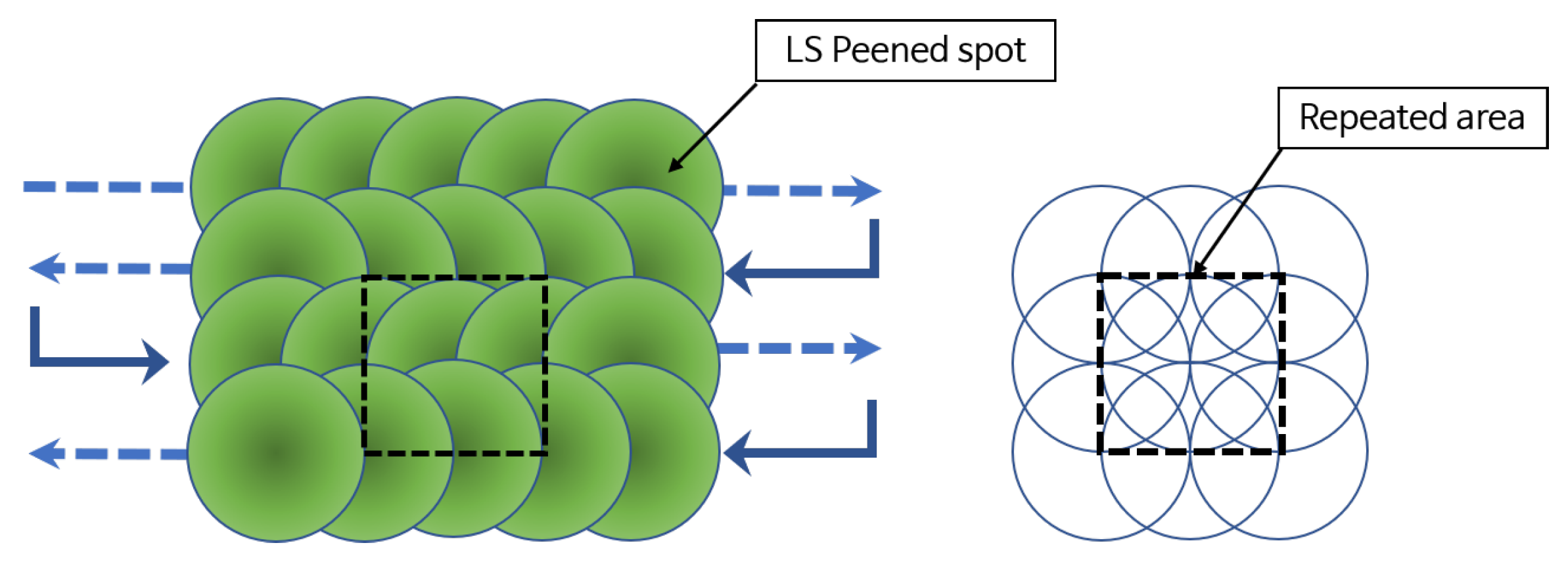
2.5. Overlapped Multiple LSP

LSP is usually performed by overlapping each single laser pulse. In this work, the laser beam was overlapped by 50% in the horizontal and vertical direction, as shown in Figure 3.

Through these repeated shots, the dotted box area appears repeatedly. To reduce the computational time, nine shots of LSP pressure loads were applied and the cross-section of the repeated area was evaluated.

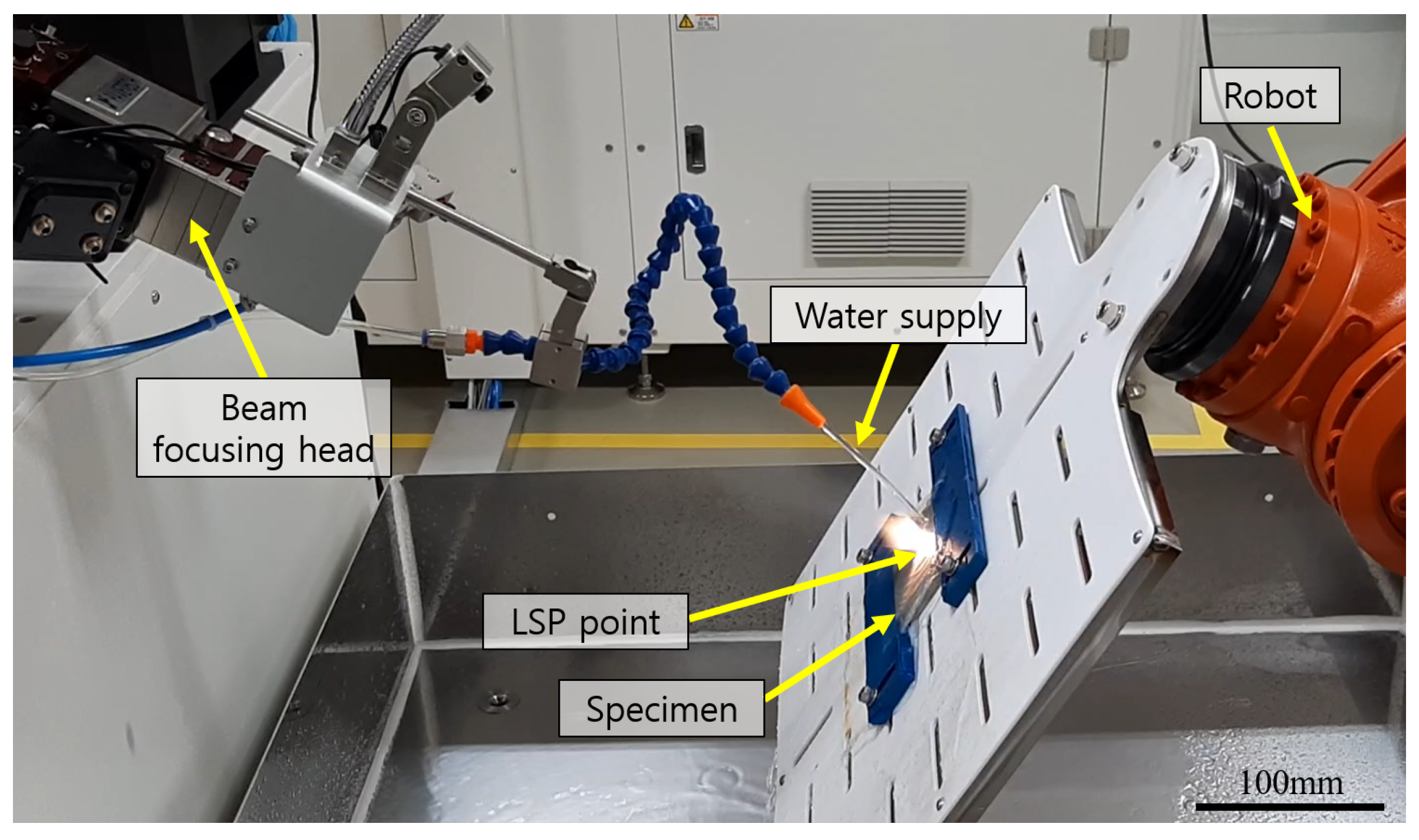
3. Experiment and FE Analysis Condition

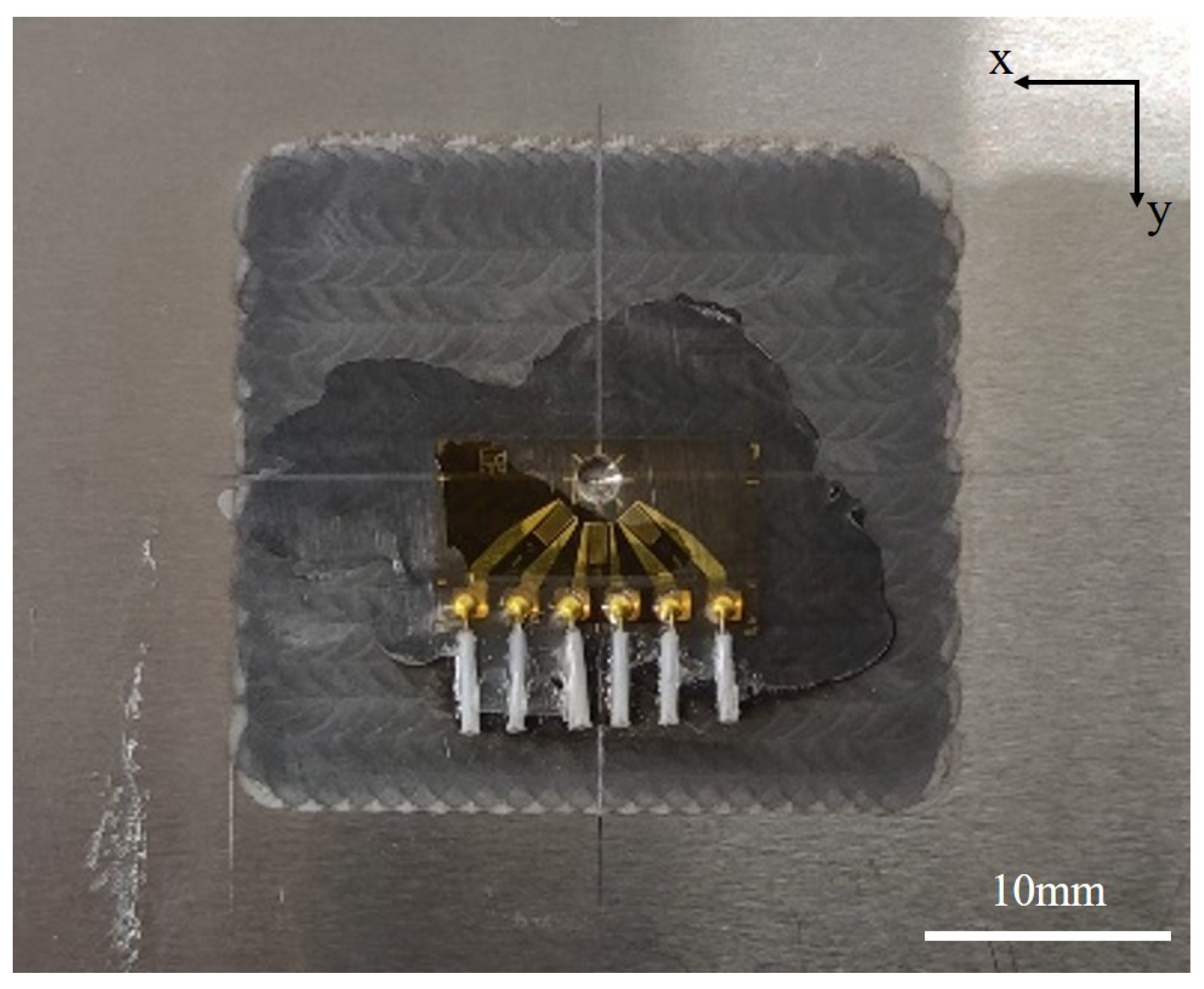
3.1. LSP Experiment Setup

In order to verify the FE simulation results, the LSP experiment was performed with the conditions shown in Table 1.

Continuum Powerlite Furie was used as a laser system, the laser pulse energy was measured by Gentec-EO Maestro console with QE65LP-H-MB-QED-D0 energy detector and the beam diameter was checked by a burn paper pattern with low-level pulse energy at the working distance. An actual LSP experimental setup is shown in Figure 4. The beam-focusing head focuses a 20 mm diameter input beam to increase the energy density, and the laser spot size can be adjusted depending on the working distance. The robot made the specimen move and water was supplied near the laser irradiation point to form the 1 mm thickness of the confinement layer. The specimen dimensions were 70 × 50 × 10 mm and the surface was ground condition.

3.2. LSP FE Simulation Setup

ANSYS Autodyn was used for LSP FE simulation and for the explicit dynamic analysis. The coordinate system, pressure loading and boundary condition faces are shown in Figure 5.

The dimension of the geometry was 20 × 20 × 5 mm, the x–y plane was parallel to the top plane of the geometry, and the z-axis was parallel to the thickness direction. The nine yellow-colored circles indicate the faces where the pressure loads were to be applied according to the LSP process model setting and the 5 faces (bottom and four lateral faces) shown in red were set to the non-reflecting boundary condition. This allowed propagating traveling waves in the outward direction of the geometry so that the energy did not reflect back into the FE geometry [13,14].

The edges of the circles where pressure loads were applied were evenly divided into 72 and the element size was set to 0.15 mm for fine mesh generation, as shown in Figure 5. For the region were pressure loads were not applied, the multi-zone meshing method was employed to generate a coarse mesh with a size of 0.25 mm. The material properties are listed in

Table 2. Material constants of STS304 and coefficients for JC model.

Material	Density	Poisson’s Ratio	Young’s Modulus	A	B	C	n	$\dot{{\mathit{\epsilon }}_0}$
	(Kg/m${}^3$)		(GPa)	(MPa)	(MPa)	(MPa)		(${\mathit{s}}^{-1}$)
STS304	7750	0.31	207	310	100	0.07	0.65	1

[32].

To apply overlapped pressure loads on the surface, the surfaces were divided into 40 regions. The pressure loads were applied in sequence as shown in Figure 6. For example, in the case of the yellow-colored surface No. 16 in Figure 6, in total, four pressure loads needed to be applied. If the laser pulse period was 10 $\mathsf{\mu }$s, the loads were applied 1st ($t=0$), 2nd ($t=10$ $\mathsf{\mu }$s), 5th ($t=40$ $\mathsf{\mu }$s) and 6th ($t=50$ $\mathsf{\mu }$s). However, each number in Figure 6 is given for convenience and is independent of the order of the loading sequence.

The static damping value was calculated from Equation (5) by solving the FE model without static damping. The time step size $\Delta t$ was $1.4\times {10}^{-10}$ from the solver output and the T was estimated to be 6 $\mathsf{\mu }\mathrm{s}$ from the energy summary in Figure 7. In this study, $R_d$ values of 0, $4.6\times {10}^{-5}$ and others were chosen to compare how the static damping affected the result of the deformation and minimum principal stress distribution. Each pressure loading period was set to 10 $\mathsf{\mu }$s.

4. Results and Discussion

4.1. Single LSP FE Analysis

4.1.1. Energy Summary

Figure 7 shows the each energy variation according to time. The total energy of the pressure pulse load was converted into the internal energy, kinetic energy and hourglass energy. Hourglass energy cannot exist in practice, but for calculation stability, it exists when solving the problem of deformation with high velocities [13]. In order to estimate the stabilization time depending on the static damping value $R_d$, the derivative of internal energy with time was plotted. In the case of the static damping $R_d$ = 0, it converged to zero with vibration. The stabilization time for the no-damping model was assumed to be 10 $\mathsf{\mu }$s, and for multiple LSP simulation, the period of each single shot was also set to 10 $\mathsf{\mu }$s. This is because, at 10 $\mathsf{\mu }$s on the kinetic energy graph, the remaining kinetic energy is relatively small, compared to the kinetic energy converted from the pressure loading instance. If the remaining kinetic energy affects the multiple LSP simulation, the solution of the no-damping model can diverge or the result may be significantly different from others. In the case of $R_d=4.6\times {10}^{-5}$, the variation in internal energy was observed before 6 $\mathsf{\mu }$s but it later converged to zero. For $R_d=50\times {10}^{-5}$, it only took 2 $\mathsf{\mu }$s to become stabilized without variation in the internal energy. Hasser et al. [17] also reported that the kinetic energy decreases quickly as damping increases. The model without damping showed the largest internal energy. The reason for this is that the applied pressure load was mostly converted into internal and kinetic energy without energy loss due to static damping.

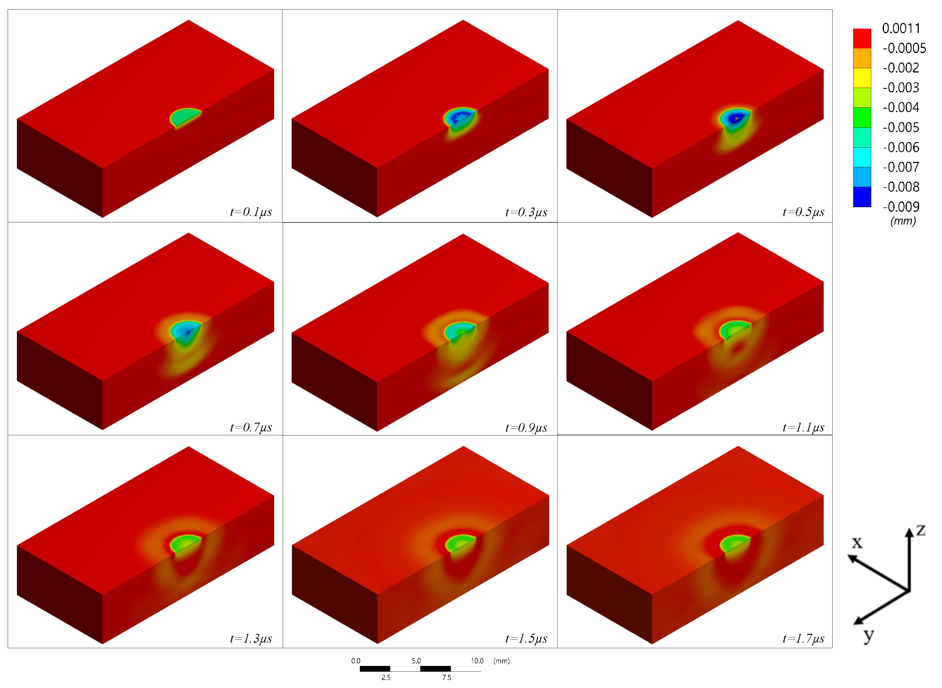
4.1.2. Transient Analysis

Since the LSP is achieved within a few microseconds, the LSP process can be visualized by performing transient analysis. Figure 8 shows the z-directional deformation of the no-damping model at every 0.2 $\mathsf{\mu }$s. A pressure load was delivered to the geometry within 0.17 $\mathsf{\mu }$s, as shown in Figure 2. However, deformation due to the pressure load was continued even afterwards. After pressure loading, the maximum amount of deformation appeared at $t=0.5$ $\mathsf{\mu }$s, and the geometry was deformed continuously in the downward direction. After 1.1 $\mathsf{\mu }$s, plastic deformation was completed and vibration was gradually reduced.

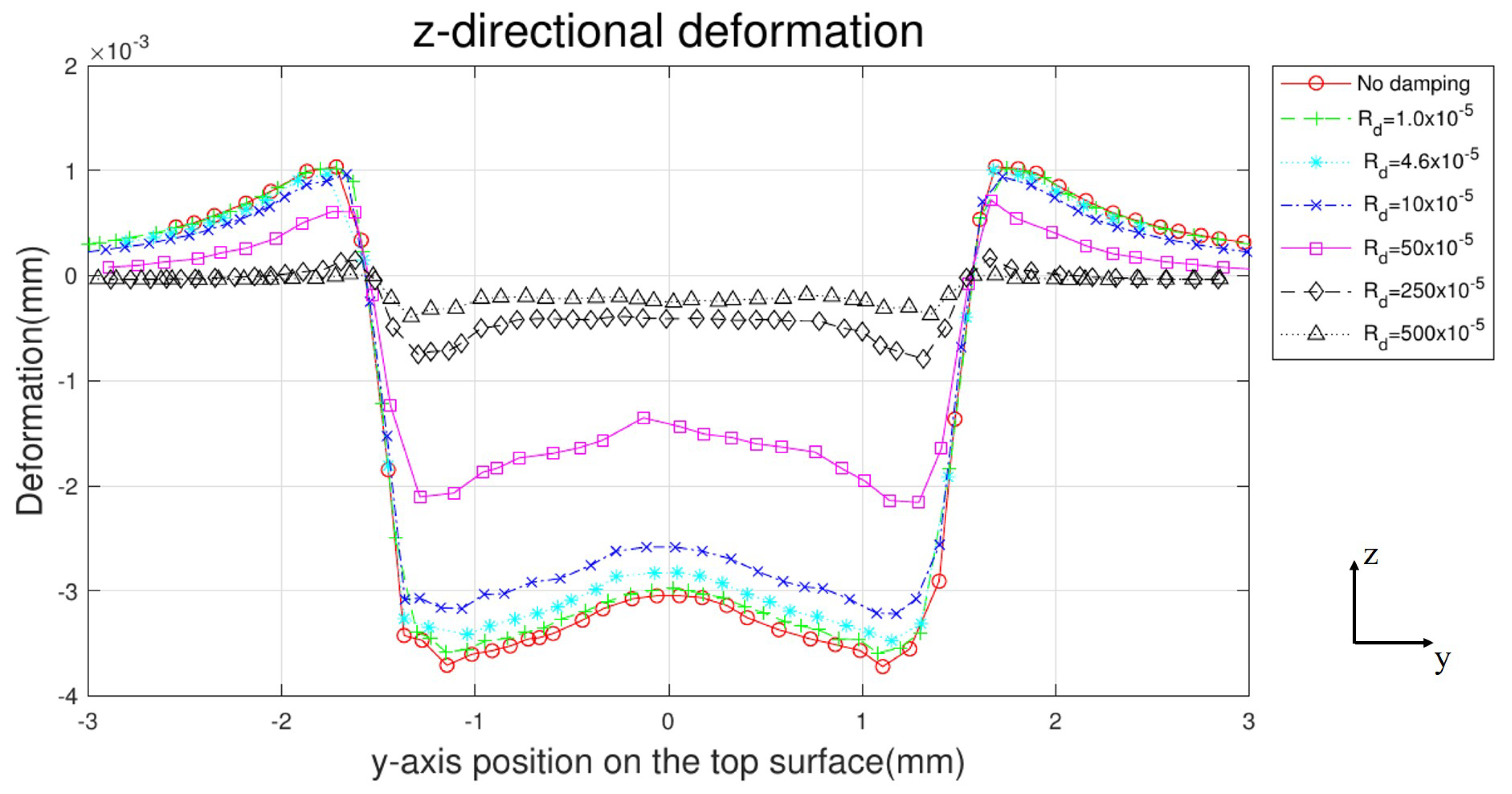
4.1.3. Deformation Distribution

To evaluate the z-directional deformation depending on the $R_d$ values, the cross-sections of the middle of the geometry were plotted as in Figure 9. In the case of a large damping value, relatively small deformation was observed. In addition, z-directional deformation values were sampled at the top of the surface. As shown in Figure 10, the center of the LSP was slightly less deformed than the surrounding area, and the surface next to the region where the pressure load was applied showed small deformation in the opposite direction.

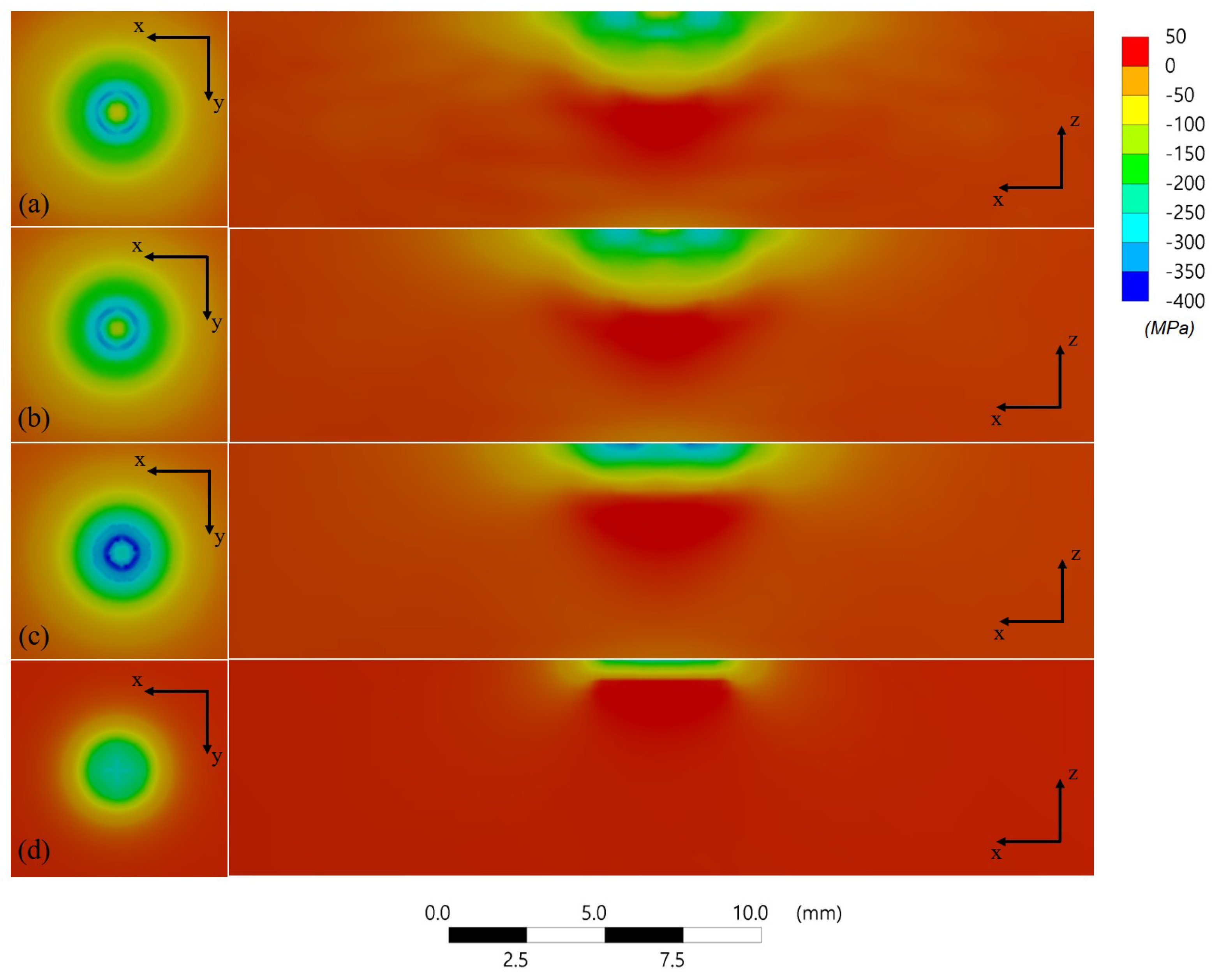
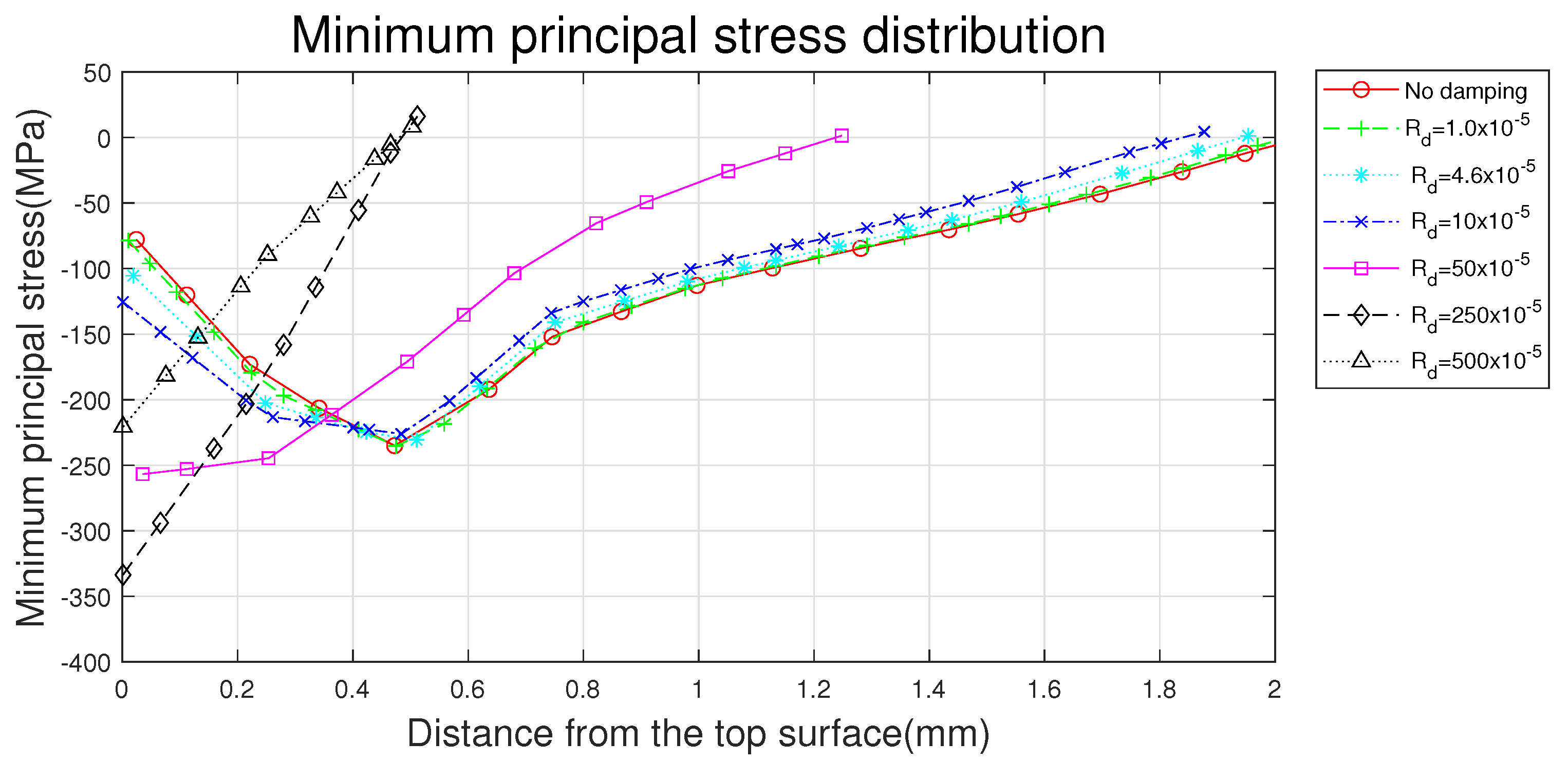
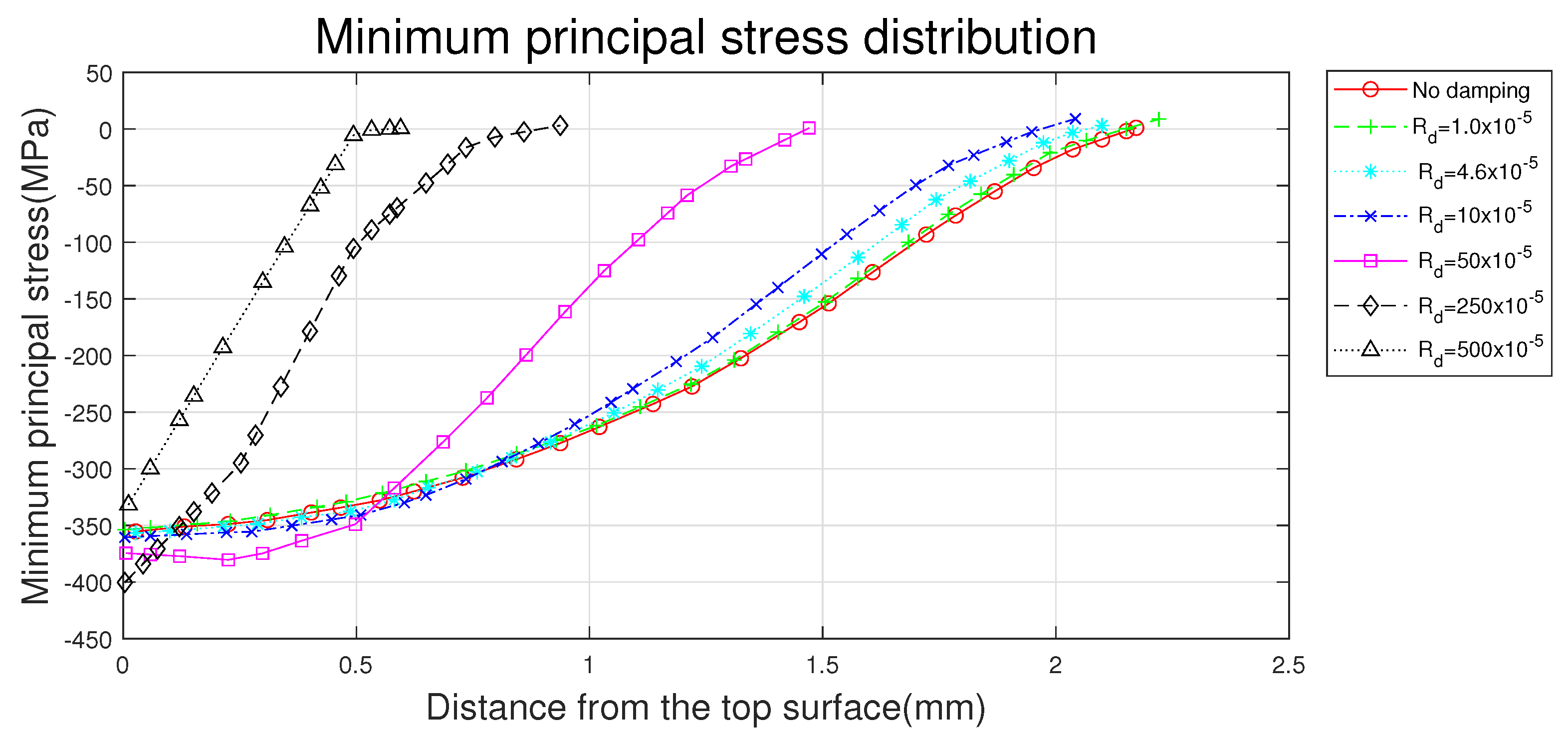
4.1.4. Minimum Principal Stress Distribution

When overlapped and complicated multiple LSP are simulated, a scalar invariant quantity such as minimum principal stress is the best practice to derive meaningful information from simulation [18]. The minimum principal stress distribution of the cross-sections was captured as shown in Figure 11. To compare the damping effect, the minimum principal stress value was sampled in the depth direction from the center point of the LSP, and it is plotted in Figure 12. Large compressive stress was formed on the surface in the case of large damping values but was relatively shallow. In contrast, deep compressive stress was achieved in the cases in which no or small damping is used. Exceptionally, from Figure 11d, only a small amount of compressive stress remained near the surface. This is due to the large damping, which significantly reduced the energy converted from the pressure load.

4.1.5. Discussion on Single LSP FE Analysis

As shown by the energy summary in Figure 7, when a large static damping value was used, the kinetic energy was quickly dissipated and, as a result, a relatively small amount of deformation was observed. It was also expected that kinetic energy would be concentrated on the surface not being transferred in the depth direction during a short period of time, and relatively large minimum principal stress was intensively formed near the surface.

Table 3. Simulation result differences depending on the static damping.

Static Damping Value ($\times {10}^{-5}$)	Time for Stabilization	Maximum Depth of Minimum Principal Stress	Maximum Deformation on the Surface
0	1.00	1.00	1.00
1	0.90	0.95	0.97
4.6	0.61	0.90	0.94
10	0.50	0.87	0.86
50	0.20	0.57	0.58
250	0.10	0.24	0.21
500	0.06	0.22	0.10

and Figure 13 show the static damping effect on the single LSP simulation result. For ease of comparison, all values were normalized based on the result of $R_d=0$. As expected, when the damping value was increased in the simulation, the model could quickly stabilize but the difference in the deformation and minimum principal stress result became larger compared to the in the case of $R_d=0$. With $R_d=4.6\times {10}^{-5}$, the simulation time could be reduced to 60% within a 10% difference from the no-damping result. This means that the static damping value $R_d=4.6\times {10}^{-5}$ evaluated from Equation (5) was reasonable. Appropriate static damping can be effective when performing multiple LSP simulation because it can reduce the calculation time for every individual shot.

4.2. Multiple LSP FE Analysis

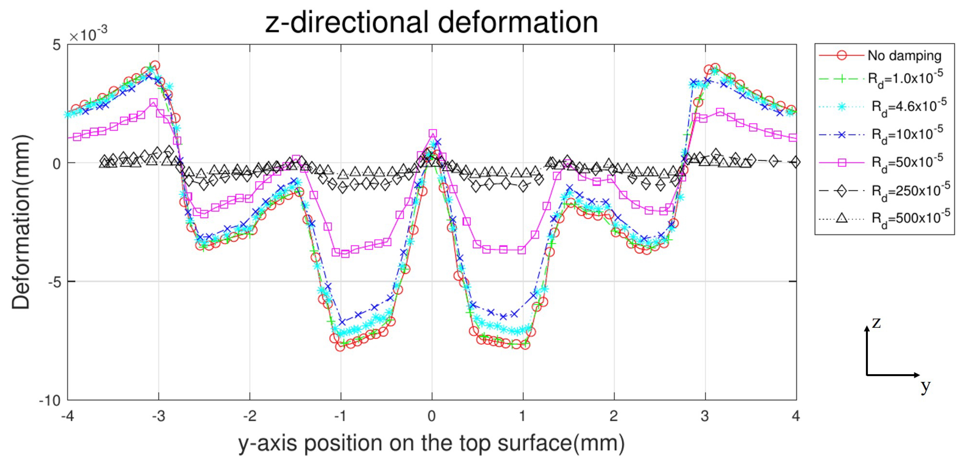
4.2.1. Deformation Distribution

Z-directional deformation values were sampled in the same manner as single LSP analysis. As shown in Figure 14 and Figure 15, faces No. 10, 16, 25 and 32 were the most deformed because of the four-times overlapped pressure loads. Similar to the single LSP result, as the damping value was increased, the amount of deformation was decreased.

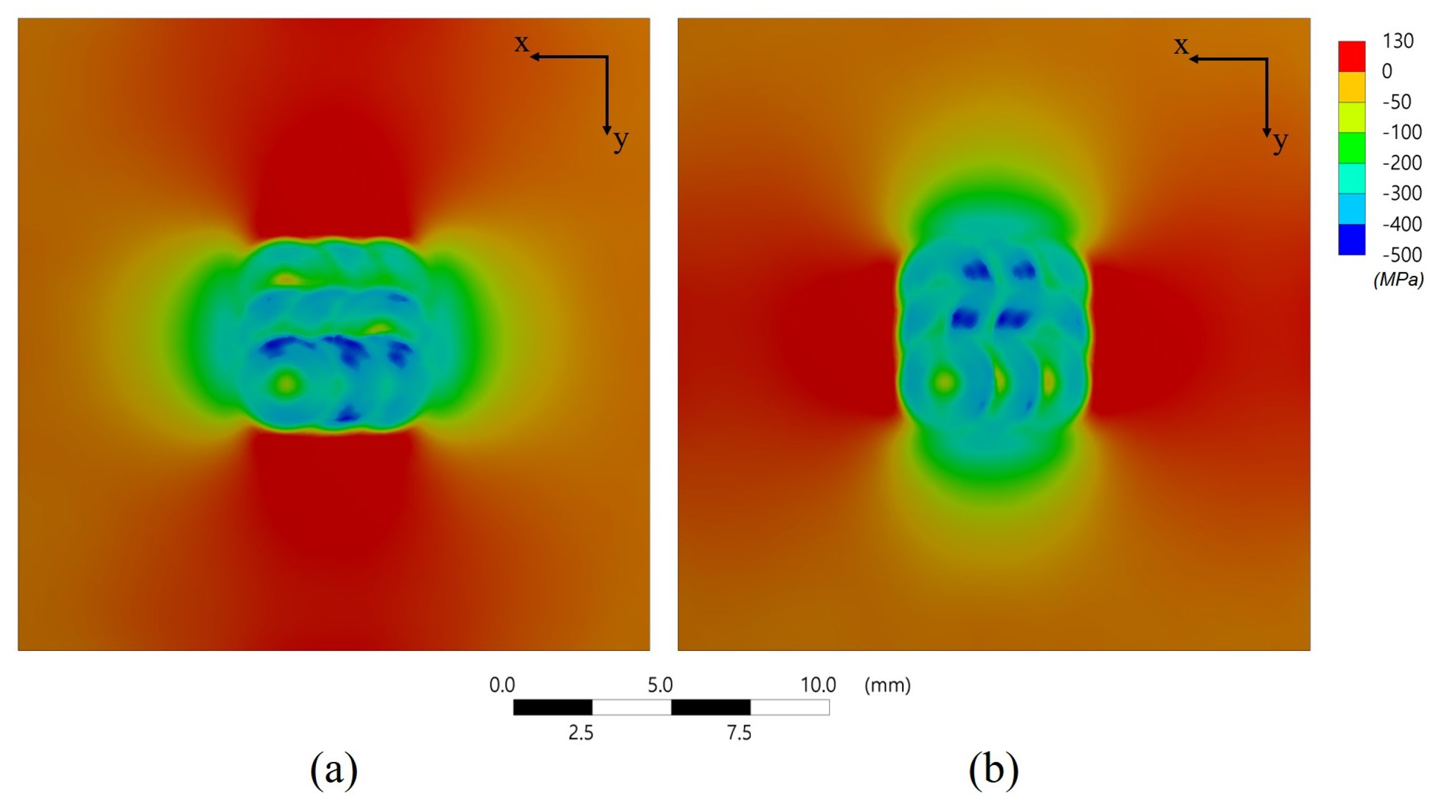
4.2.2. Minimum Principal Stress Distribution

The minimum principal stress distribution of the multiple LSP FE simulation is shown in Figure 16 and Figure 17. In the case of a large value of static damping, even though the pressure loads were overlapped, minimum principal stress was not formed deeply but was formed intensively near the surface of the geometry.

In the multiple LSP FE simulation, the effect of the static damping was similar to the single LSP simulation. As the pressure loads were overlapped, the amount of deformation and the minimum principal stress were increased. In other words, the laser pulses should be overlapped to maximize the LSP effect.

From the deformation and the stress analysis results, the no-damping simulation was not diverged and the result was not significantly different from the others. This means that even though there exists a small kinetic energy in the model, it does not significantly effect the solution of the LSP simulation.

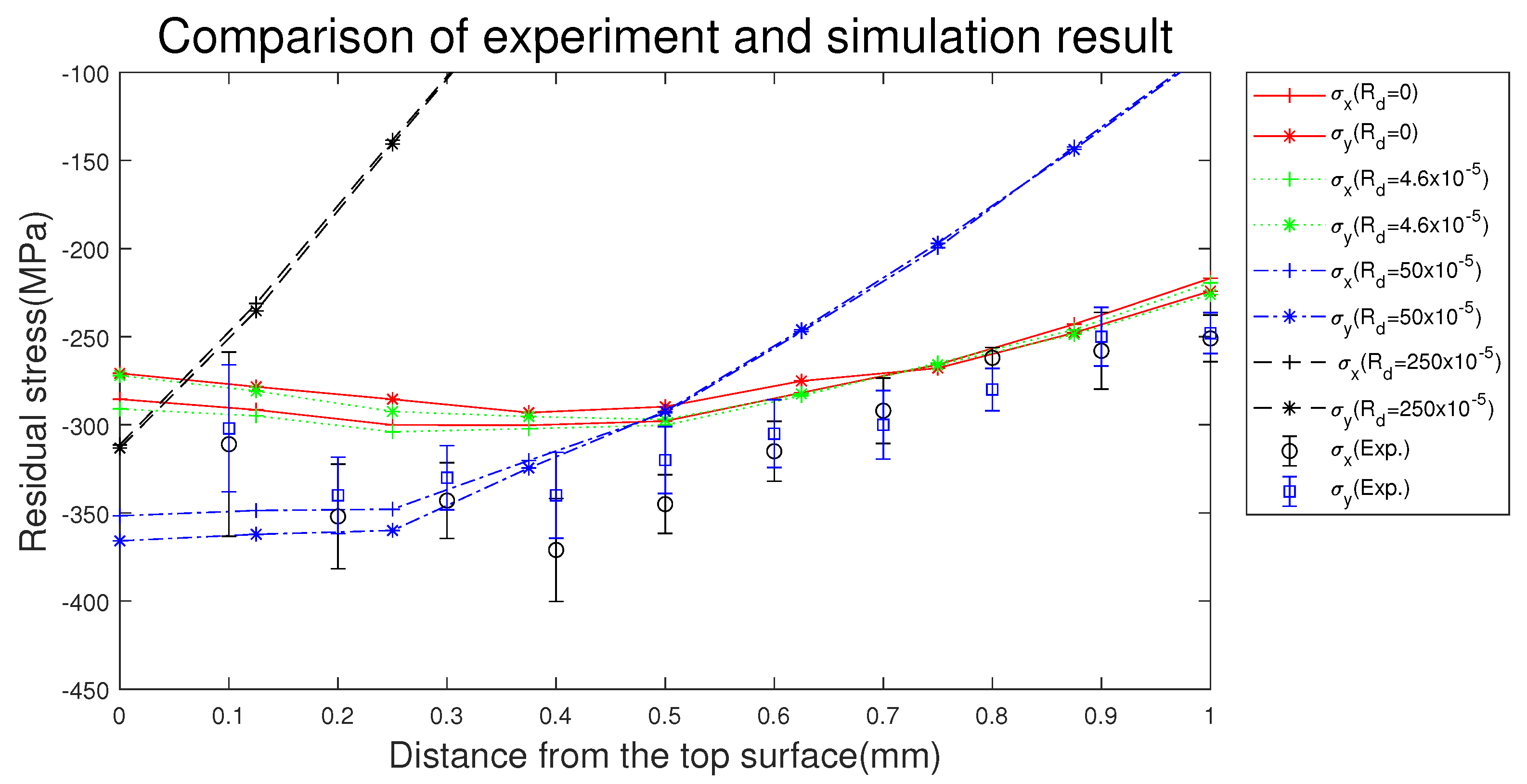
4.3. Residual Stress Distribution of LSP Material

To verify the simulation results, the residual stress of the actual LSP-treated specimen was measured by the hole drilling method as shown in Figure 18. The main purpose of the LSP experiment was to determine whether the compressive residual stress was formed up to a depth of 1 mm. Accordingly, the residual stress was measured up to 1 mm in the depth direction at the center of the LSP test specimen. The measurement conditions are listed in

Table 4. Hole drilling test parameters for residual stress measurement.

Material	Analysis Method	Hole Step	Step Method	Hole Depth (mm)	Analysis Step	Analysis Step Method	Analysis Depth (mm)	Drill dia. (mm)
STS304	ASTM E837-13	24	Linear	1.2	20	Linear	1	1.6

.

To derive the residual stress, normal stress ${\sigma }_x$ and ${\sigma }_y$ were analyzed. Figure 19 shows the residual stress distribution on the solution geometry surface. The residual stress evaluated from the simulation was not evenly distributed. On the other hand, in-plane residual stresses from the hole drilling method within a certain region are assumed to be constant. Keller et al. [33] averaged the nodal stresses in the laser shock peened area from the top surface to the depth direction. Similarly, the residual stress in the dotted area shown in Figure 3 was averaged at every 0.125 mm in the depth direction for comparison with the hole drilling result.

The residual stress(${\sigma }_x$ and ${\sigma }_y$) of the specimen and the simulation according to depth are plotted in Figure 20. The figure shows that the distribution of compressive residual stress in both the FE simulation and the experiment were similar to each other, in the case of $R_d=0$ and $R_d=4.6\times {10}^{-5}$. The residual stress distribution expressed as ${\sigma }_x$ and ${\sigma }_y$ in the depth direction was not significantly different from the minimum principal stress.

The residual stress distribution ${\sigma }_x$ and ${\sigma }_y$ showed a small anisotropic relationship, as shown in Figure 20. Kallien et al. [34] reported that, depending on the overlap and sequence of laser shots, a non-equibiaxial residual stress distribution can be observed in AA2024-T3 material. The mechanism of anisotropic stress generation in LSP of ferrite–pearlite steel was reported by Hirano et al. [35]. Depending on the laser pulse irradiation sequence and the pattern, residual stress distribution can be isotropic or anisotropic. Hirano et al. introduced the coverage ratio term, which is expressed as Equation (9).

$$C=\frac{N(\pi D^2/4)}{S}$$

(9)

C is the coverage ratio, N is the total number of laser pulses irradiated, D is the spot diameter and S is the LSP processed area. When $C>2$, LSP stress tends to be anisotropic. In other words, the laser pulses are densely irradiated within the unit area, and the difference between ${\sigma }_x$ and ${\sigma }_y$ becomes larger. A similar relationship was observed in stainless steel 304 [36]. In this study, the coverage ratio C could be calculated to be 1.77 from the LSP parameters, and it indicates that there was a small non-equibiaxial residual stress distribution.

5. Conclusions

In this study, LSP FE simulation was performed and both deformation and the residual stress were evaluated. The simulation result was also compared with the LSP experiment specimen to determine whether the proposed simulation process is appropriate. The study can be summarized as follows:

• The single and multi-shot explicit dynamic LSP FE analysis was conducted with the proposed static damping model by ANSYS Autodyn.
• An implicit analysis that involved stabilizing the geometry can be skipped by adding the static damping value.
• The static damping quickly settles the model after shock loading, but with large damping, residual stress is formed near the surface of the geometry, albeit not deeply, and relatively small plastic deformation can be obtained.
• A comparison of residual stress measurement results on the LSP specimen with compressed residual stress obtained from the simulation showed a similar tendency.
• The residual stress of the FE simulation and that measured by hole drilling showed a small anisotropic relationship due to the LSP process parameters.
• By using the proper static damping value in LSP FE simulation, the calculation time can be reduced and there is no significant effect on the simulation result.

Compared to other peening methods, LSP is a high-cost material surfacing process. To evaluate the actual residual stress distribution, additional destructive tests such as hole drilling are also required. Therefore, when quick verification of the residual stress distribution is needed according to the depth formed by the LSP, the proposed FE simulation model can be appropriate.

References

1. Ding, K.; Ye, L. Laser Shock Peening: Performance and Process Simulation; Woodhead Publishing: Sawston, UK, 2006. [Google Scholar]
2. Lu, J.Z.; Luo, K.Y.; Yang, D.K.; Cheng, X.N.; Hu, J.L.; Dai, F.Z.; Qi, H.; Zhang, L.; Zhong, J.S.; Wang, Q.W.; et al. Effects of laser peening on stress corrosion cracking (SCC) of ANSI 304 austenitic stainless steel. Corros. Sci. 2012, 60, 145–152. [Google Scholar] [CrossRef]
3. Telang, A.; Gill, A.S.; Teysseyre, S.; Mannava, S.R.; Qian, D.; Vasudevan, V.K. Effects of laser shock peening on SCC behavior of Alloy 600 in tetrathionate solution. Corros. Sci. 2015, 90, 434–444. [Google Scholar] [CrossRef] [Green Version]
4. Grethlein, J.E. Keep Em Flying Laser Peening Keeps Aircraft Turbine Blades in Action. AMPTIAC Q. 2003, 7, 3–7. [Google Scholar]
5. Kim, J.D.; SANO, Y. Laser Peening Application for PWR Power Plants. J. Weld. Join. 2016, 34, 13–18. [Google Scholar] [CrossRef]
6. Braisted, W.; Brockman, R. Finite element simulation of laser shock peening. Int. J. Fatigue 1999, 21, 719–724. [Google Scholar] [CrossRef]
7. Asghar, M.H.; Placido, F.; Naseem, S. P HYSICAL J OURNAL Characterization of reactively evaporated TiO2 thin films as high. Eur. Phys. J. Appl. Phys. 2006, 184, 177–184. [Google Scholar] [CrossRef]
8. Peyre, P.; Chaieb, I.; Braham, C. FEM calculation of residual stresses induced by laser shock processing in stainless steels. Model. Simul. Mater. Sci. Eng. 2007, 15, 205–221. [Google Scholar] [CrossRef]
9. Amarchinta, H.K.; Grandhi, R.V.; Langer, K.; Stargel, D.S. Material model validation for laser shock peening process simulation. Model. Simul. Mater. Sci. Eng. 2009, 17, 015010. [Google Scholar] [CrossRef]
10. Amarchinta, H.K.; Grandhi, R.V.; Clauer, A.H.; Langer, K.; Stargel, D.S. Simulation of residual stress induced by a laser peening process through inverse optimization of material models. J. Mater. Process. Technol. 2010, 210, 1997–2006. [Google Scholar] [CrossRef]
11. Hfaiedh, N.; Peyre, P.; Song, H.; Popa, I.; Ji, V.; Vignal, V. Finite element analysis of laser shock peening of 2050-T8 aluminum alloy. Int. J. Fatigue 2015, 70, 480–489. [Google Scholar] [CrossRef] [Green Version]
12. Li, X.; He, W.; Luo, S.; Nie, X.; Tian, L.; Feng, X.; Li, R. Simulation and experimental study on residual stress distribution in titanium alloy treated by laser shock peening with flat-top and Gaussian laser beams. Materials 2019, 12, 1343. [Google Scholar] [CrossRef] [Green Version]
13. Hu, Y.; Yao, Z.; Hu, J. 3-D FEM simulation of laser shock processing. Surf. Coat. Technol. 2006, 201, 1426–1435. [Google Scholar] [CrossRef]
14. Hu, Y.; Yao, Z. Numerical simulation and experimentation of overlapping laser shock processing with symmetry cell. Int. J. Mach. Tools Manuf. 2008, 48, 152–162. [Google Scholar] [CrossRef]
15. Bhamare, S.; Ramakrishnan, G.; Mannava, S.R.; Langer, K.; Vasudevan, V.K.; Qian, D. Simulation-based optimization of laser shock peening process for improved bending fatigue life of Ti-6Al-2Sn-4Zr-2Mo alloy. Surf. Coat. Technol. 2013, 232, 464–474. [Google Scholar] [CrossRef]
16. Ballard, P.; Fournier, J.; Fabbro, R.; Frelat, J. Residual Stresses Induced by Laser-Shocks. J. Phys. IV 1991, 1, C3-487–C3-494. [Google Scholar] [CrossRef]
17. Hasser, P.J.; Malik, A.S.; Langer, K.; Spradlin, T.J.; Hatamleh, M.I. An Efficient Reliability-Based Simulation Method for Optimum Laser Peening Treatment. J. Manuf. Sci. Eng. Trans. ASME 2016, 138, 111001. [Google Scholar] [CrossRef]
18. Brockman, R.A.; Braisted, W.R.; Olson, S.E.; Tenaglia, R.D.; Clauer, A.H.; Langer, K.; Shepard, M.J. Prediction and characterization of residual stresses from laser shock peening. Int. J. Fatigue 2012, 36, 96–108. [Google Scholar] [CrossRef]
19. Fameso, F.; Desai, D.; Kok, S.; Newby, M.; Glaser, D.; Fameso, F. Coupled explicit-damping simulation of laser shock peening on x12Cr steam turbine blades. J. Phys. Conf. Ser. 2021, 1780, 012002. [Google Scholar] [CrossRef]
20. ANSYS. Chapter 6, Explicit Dynamics Theory Guide; ANSYS, Inc.: Canonsburg, PA, USA, 2009. [Google Scholar]
21. ANSYS. Chapter 8, Explicit Dynamics Analysis Settings; ANSYS, Inc.: Canonsburg, PA, USA, 2009. [Google Scholar]
22. ANSYS. ANSYS Explicit Dynamics Analysis Guide; ANSYS, Inc.: Canonsburg, PA, USA, 2020; p. 394. [Google Scholar]
23. Johnson, G.R.; Cook, W. A constitutive model and data for metals subjected to large strains, high strain rates and high temperatures. In Proceedings of the 7th International Symposium on Ballistics, Hague, The Netherlands, 19–21 April 1983; pp. 541–547. [Google Scholar]
24. Zerilli, F.J.; Armstrong, R.W. Dislocation-mechanics-based constitutive relations for material dynamics calculations. J. Appl. Phys. 1998, 61, 1816. [Google Scholar] [CrossRef] [Green Version]
25. Khan, A.S.; Suh, Y.S.; Kazmi, R. Quasi-static and dynamic loading responses and constitutive modeling of titanium alloys. Int. J. Plast. 2004, 20, 2233–2248. [Google Scholar] [CrossRef]
26. Karkalos, N.E.; Markopoulos, A.P. Determination of Johnson-Cook material model parameters by an optimization approach using the fireworks algorithm. Procedia Manuf. 2018, 22, 107–113. [Google Scholar] [CrossRef]
27. Langer, K.; Spradlin, T.J.; Fitzpatrick, M.E. Finite element analysis of laser peening of thin aluminum structures. Metals 2020, 10, 93. [Google Scholar] [CrossRef] [Green Version]
28. Nam, T. Finite Element Analysis of Residual Stress Field Induced by Laser Shock Peening. Ph.D. Thesis, Ohio State University, Columbus, OH, USA, 2002. [Google Scholar]
29. Kim, J.S.; Nam, H.S.; Kim, Y.J.; Kim, J.H. Numerical Study of Laser Shock Peening Effects on Alloy 600 Nozzles with Initial Residual Stresses. J. Press. Vessel Technol. Trans. ASME 2017, 139, 1–8. [Google Scholar] [CrossRef]
30. Berthe, L.; Fabbro, R.; Peyre, P.; Tollier, L.; Bartnicki, E. Shock waves from a water-confined laser-generated plasma. J. Appl. Phys. 1997, 82, 2826–2832. [Google Scholar] [CrossRef]
31. Sun, B.; Qiao, H.; Zhao, J. Accurate numerical modeling of residual stress fields induced by laser shock peening. AIP Adv. 2018, 8, 095203. [Google Scholar] [CrossRef] [Green Version]
32. Espinosa, H.D.; Lee, S.; Moldovan, N. A novel fluid structure interaction experiment to investigate deformation of structural elements subjected to impulsive loading. Exp. Mech. 2006, 46, 805–824. [Google Scholar] [CrossRef]
33. Keller, S.; Chupakhin, S.; Staron, P.; Maawad, E.; Kashaev, N.; Klusemann, B. Experimental and numerical investigation of residual stresses in laser shock peened AA2198. J. Mater. Process. Technol. 2018, 255, 294–307. [Google Scholar] [CrossRef]
34. Kallien, Z.; Keller, S.; Ventzke, V.; Kashaev, N.; Klusemann, B. Effect of Laser Peening Process Parameters and Sequences on Residual Stress Profiles. Metals 2019, 9, 655. [Google Scholar] [CrossRef] [Green Version]
35. Hirano, K.; Sugihashi, A.; Imai, H.; Hamada, N. Mechanism of anisotropic stress generation in laser peening process. Int. Congr. Appl. Lasers Electro-Opt. 2006, 2006, P511. [Google Scholar] [CrossRef]
36. Mukai, N.; Aoki, N.; Obata, M.; Ito, A.; Sano, Y.; Konagai, C. Laser processing for underwater maintenance in nuclear plants. In Proceedings of the 3rd JSME/ASME Joint International Conference on Nuclear Engineering, Kyoto, Japan, 23–27 April 1995; Volume 3, pp. 1489–1494. [Google Scholar]
Figure 1. Analysis flow chart: (a) Typical explicit and implicit method; (b) SEATD explicit method; (c) Proposed static damping explicit method.
Metals 11 01516 g001
Figure 2. Pressure load profile; (a) Normalized pressure load profile adapted from [9,28]; (b) Plasma pressure load model induced by laser pulse, 4.2 J of pulse energy with pulse width of 10 ns.
Metals 11 01516 g002
Figure 3. Example of the overlapped multiple LSP pattern.
Metals 11 01516 g003
Figure 4. LSP experiment system setup.
Metals 11 01516 g004
Figure 5. FE model setup; (a) Pressure load and boundary condition faces; (b) Edge sizing for fine mesh generation.
Metals 11 01516 g005
Figure 6. Example of the overlapped multiple LSP pattern; (a) Pressure load timing on face No. 16; (b) Pressure loading sequence. The gray-colored dotted line indicates the laser pulse path.
Metals 11 01516 g006
Figure 7. Energy summary of solution. The differential of internal energy ( Δ E I n t e r n a l / Δ t ) is plotted to evaluate the stabilizing time for each damping value.
Metals 11 01516 g007
Figure 8. Transient analysis of the z-directional deformation in single LSP.
Metals 11 01516 g008
Figure 9. Z-directional deformation of single LSP FE solution. Top (x–y plane) and cross-section (x–z plane) view: (a) R d = 0; (b) R d = 4.6 × 10 5 ; (c) R d = 50 × 10 5 ; (d) R d = 500 × 10 5 .
Metals 11 01516 g009
Figure 10. Z-directional deformation distribution on the top surface.
Metals 11 01516 g010
Figure 11. Minimum principal stress of single LSP FE solution. Top (x–y plane) and cross-section (x–z plane) view: (a) R d = 0; (b) R d = 4.6 × 10 5 ; (c) R d = 50 × 10 5 ; (d) R d = 500 × 10 5 .
Metals 11 01516 g011
Figure 12. Minimum principal stress of single LSP FE solution in the depth (z-) direction at the center of the pressure load applied.
Metals 11 01516 g012
Figure 13. Normalized effect on the FE simulation according to static damping value.
Metals 11 01516 g013
Figure 14. Z-directional deformation of multiple LSP FE solution. Top (x–y plane) and cross-section (x–z plane) view: (a) R d = 0; (b) R d = 4.6 × 10 5 ; (c) R d = 50 × 10 5 ; (d) R d = 500 × 10 5 .
Metals 11 01516 g014
Figure 15. Z-directional deformation distribution on the top surface of multiple LSP FE solution.
Metals 11 01516 g015
Figure 16. Minimum principal stress of multiple LSP FE solution. Top (x–y plane) and cross-section (x–z plane) view: (a) R d = 0; (b) R d = 4.6 × 10 5 ; (c) R d = 50 × 10 5 ; (d) R d = 500 × 10 5 .
Metals 11 01516 g016
Figure 17. Minimum principal stress of multiple LSP FE solution in the depth (z-) direction at face No. 16 in Figure 6.
Metals 11 01516 g017
Figure 18. Residual stress measurement of the LSP specimen.
Metals 11 01516 g018
Figure 19. Residual stress of the geometry surface ( R d = 0 ): (a) normal stress σ x and (b) normal stress σ y .
Metals 11 01516 g019
Figure 20. Residual stress comparison of the experiment and simulation result in the depth (z-) direction.
Metals 11 01516 g020