Article

Fracture Areas Quantitative Investigating of Bending-Torsion Fatigued Low-Alloy High-Strength Steel

Faculty of Mechanical Engineering and Ship Technology, Gdańsk University of Technology, 11/12 Gabriela Narutowicza Street, 80-233 Gdańsk, Poland
Metals 2021, 11(10), 1620; https://doi.org/10.3390/met11101620
Submission received: 8 September 2021 / Revised: 4 October 2021 / Accepted: 9 October 2021 / Published: 12 October 2021
(This article belongs to the Special Issue High-Strength Low-Alloy Steels: Current and Future Challenges)

Abstract

:
In this study, the impact of pseudo-random non-proportional bending-torsion fatigue loadings proportion on the fatigue life and the fracture surface topography was analyzed. Investigation was carried out for 24 specimens made of S355J2 steel with 11 different ratios of maximum stresses λ. For these cases, after the fatigue tests, the surface topography measurements were carried out using an optical profilometer, using the focus variation method. Three fracture zones were analyzed for each specimen: (1) total; (2) propagation; (3) rupture, taking into account the root average square height Sq and void volume Vv parameters. The results pointed that ratio of maximum stresses λ is the most influenced on volume surface parameters represented by void volume at a given height Vv, in the rupture area. A new fatigue loading parameter P was used, depending on fatigue life T and ratio of maximum stresses λ, which shows very good correlation in 4th degree type of fit, to void volume Vv parameter for the rupture area.

1. Introduction

High-strength low-alloyed (HSLA) steels are often the optimal material due to their balanced economic properties and technical properties [1]. Especially accurate fatigue design, for the security factor on the example of the S355 steel has great importance [2]. Therefore, Cruces et al. [3] as well as Pawliczek and Rozumek [4] studied multiaxial fatigue and fracture of this type of steel in their research. The importance of this issue is indicated by a large number of publications on fatigue and fracture of HSLA steels subjected to various kind treatments [5,6].
Another field of engineering science that is very helpful in material research is surface metrology [7,8]. The industrial application of areal surface texture measurement started just in the 1990s but many comparisons of various areal surface topography measuring instruments have been published [9,10,11]. In previous research by most of the Researchers, areal surface topography was used for the manufacturing material measures [12,13,14,15]. However, surface metrology is needed not only to improve production quality, but also in many other aspects of science [16,17,18].
Surface flaws and internal cracks play a central role in the failure of materials. Therefore, fracture mechanisms are studied very widely, e.g., Wu et al. [19] presented a fatigue life prediction model considering crack propagation and closure effect. Additionally, Derpeński et al. [20] have taken up fracture tests of axisymmetric specimens with circumferential notches under elevated temperature. The fractography concerns the interconnection among surface topography of the fracture and the mechanisms as well as states conducting to their formation [21,22,23]. Therefore, it is a combination of all the aspects mentioned in this Introduction.
This paper focus on the promising results obtained by fractographical analysis, partially presented previously by the Author. One of the most important outcomes is the introduction of field parameters S- and V- in the context of the description of fatigue fracture surfaces of 6082 aluminum alloy [24], fractal dimension for bending-torsion fatigue fracture surfaces [25,26], strain sequence consequences on fracture surface topographies in 7075-T651 aluminum alloy specimens [27], or also to compare profile and areal surface parameters for fracture specifications [28]. R-profile and areal S-parameters were also taken into account in another cited work by the Author [29], to explain the effect of various fatigue variables during fracture surface formation of notched 2017A-T4 aluminum alloy under bending fatigue. However, it was decided that the entire fracture surface method was compared to other areas of the fatigue fractures after bending, torsion and a combination of these loadings. This study was carried out for a similar set of specimens as in [30].
Coming after the Introduction, the paper is organized as follows: Section 2 describes the materials and methods used for this research. Section 3 gathers information on the experimental fatigue test and fracture surface program results. Section 4 presents the discussion and main outcomes of the fatigue campaign and the fracture topography parameters, as well as their relationships. The paper ends with a summary of the most relevant findings.

2. Materials and Methods

Experimental data, with the goal of demonstrating the effect of different values of normal and shear stresses and their correlation on the fatigue life of the material as well as to verify the relationship of the fracture surface with type of fatigue loading histories, were selected similarly to [30], but taking into account other zones and the fracture surface parameters.

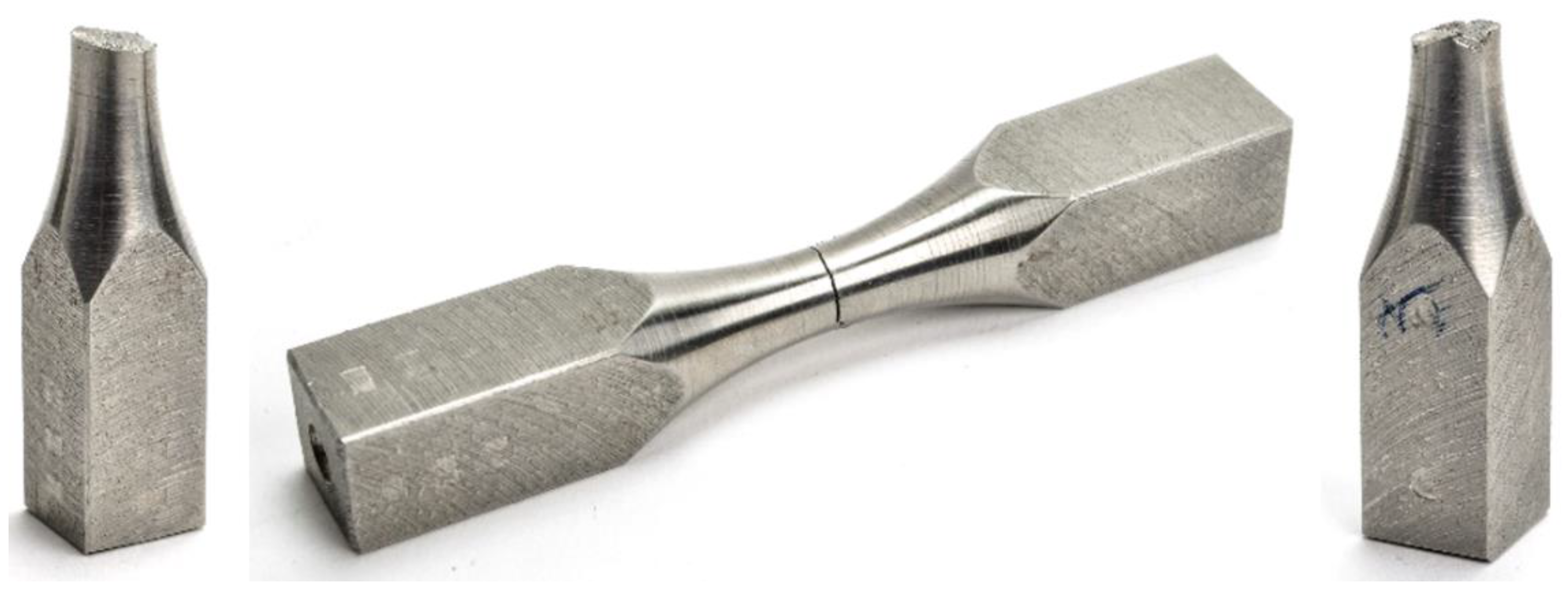
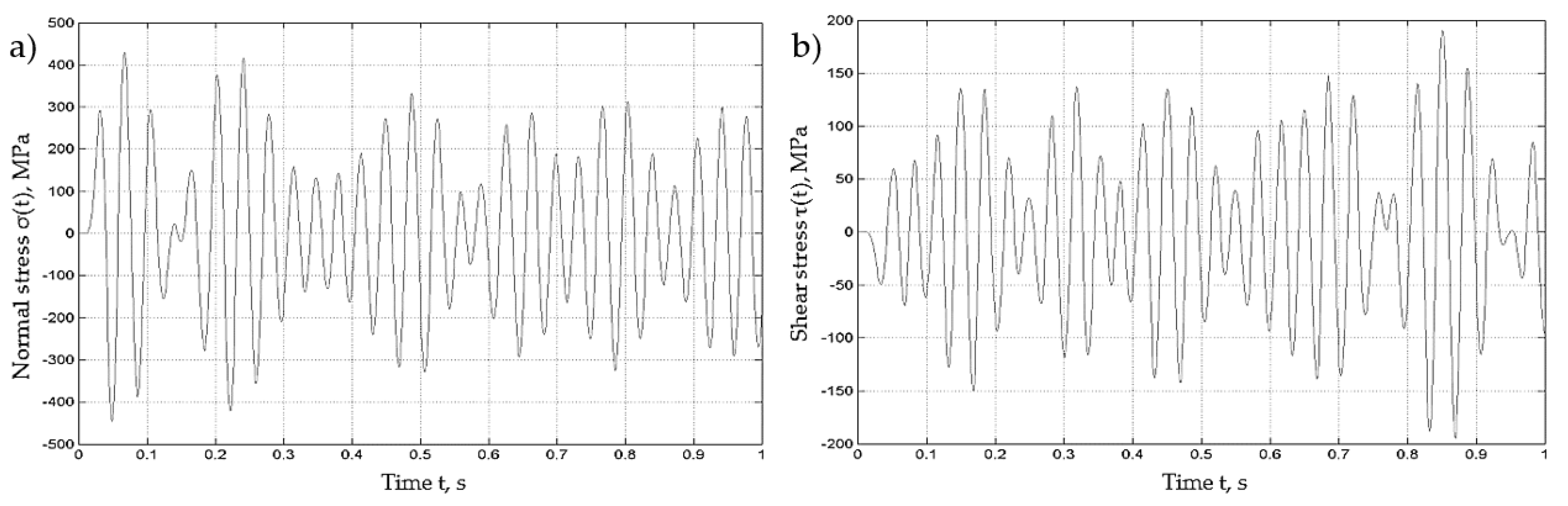
2.1. Bending-Torsion Fatigue Test

The S355J2 steel used in the paper was fatigue examined by Marciniak et al. [31,32]. Bending-torsion fatigue campaign was done using 8mm-diameter specimens illustrated in the pictures in Figure 1.
In Figure 2a,b we can see examples of non-proportional pseudorandom histories of normal stresses σ(t) and shear stresses τ(t) in time, respectively.
To present the classification of 11 combinations of loading levels, a scatter plot of maximum normal stress σmax and maximum shear stress τmax, grouped by 24 results of fatigue life T was generated (see Figure 3).

2.2. Fracture Surface Topography Measurement
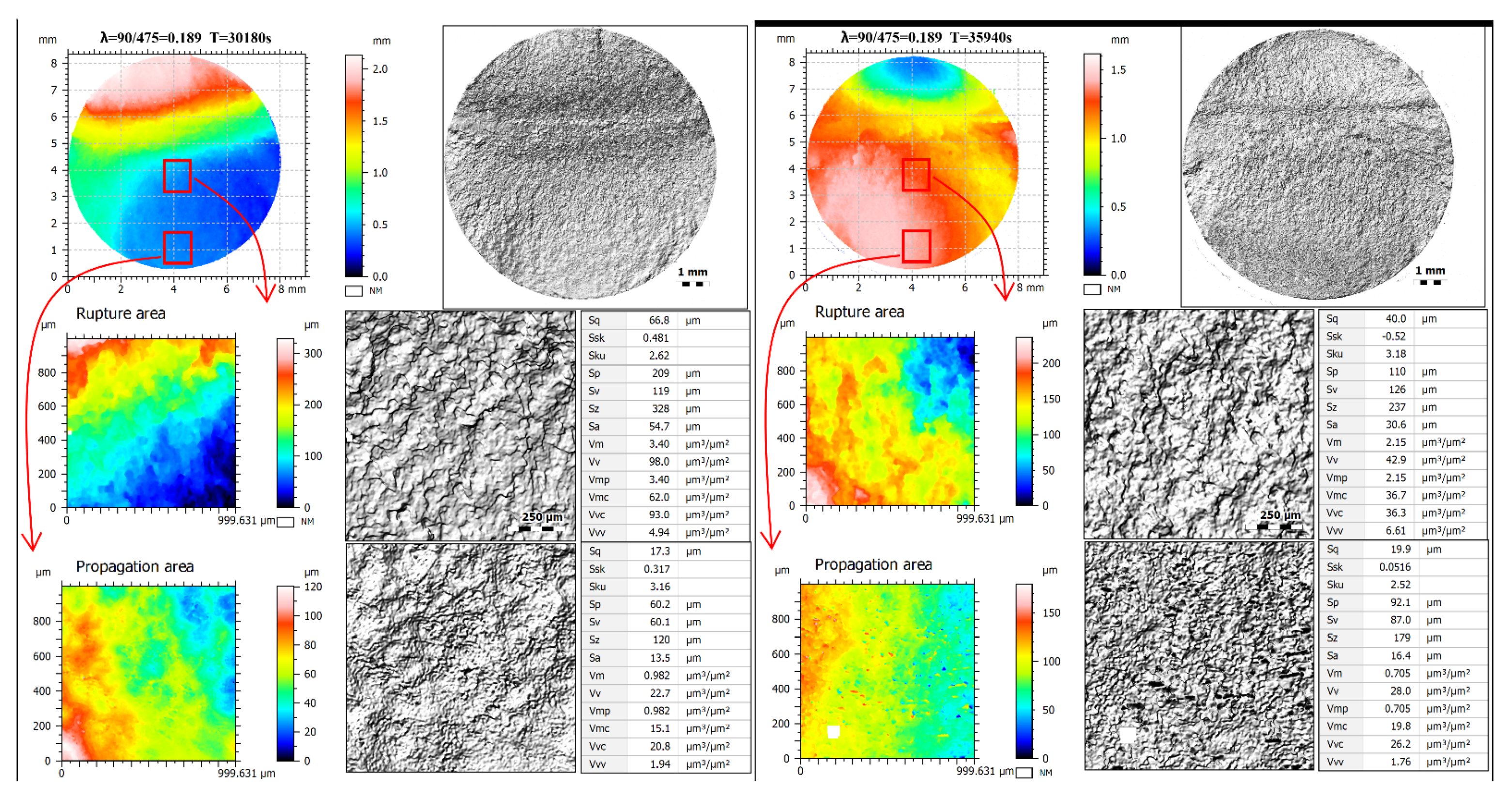
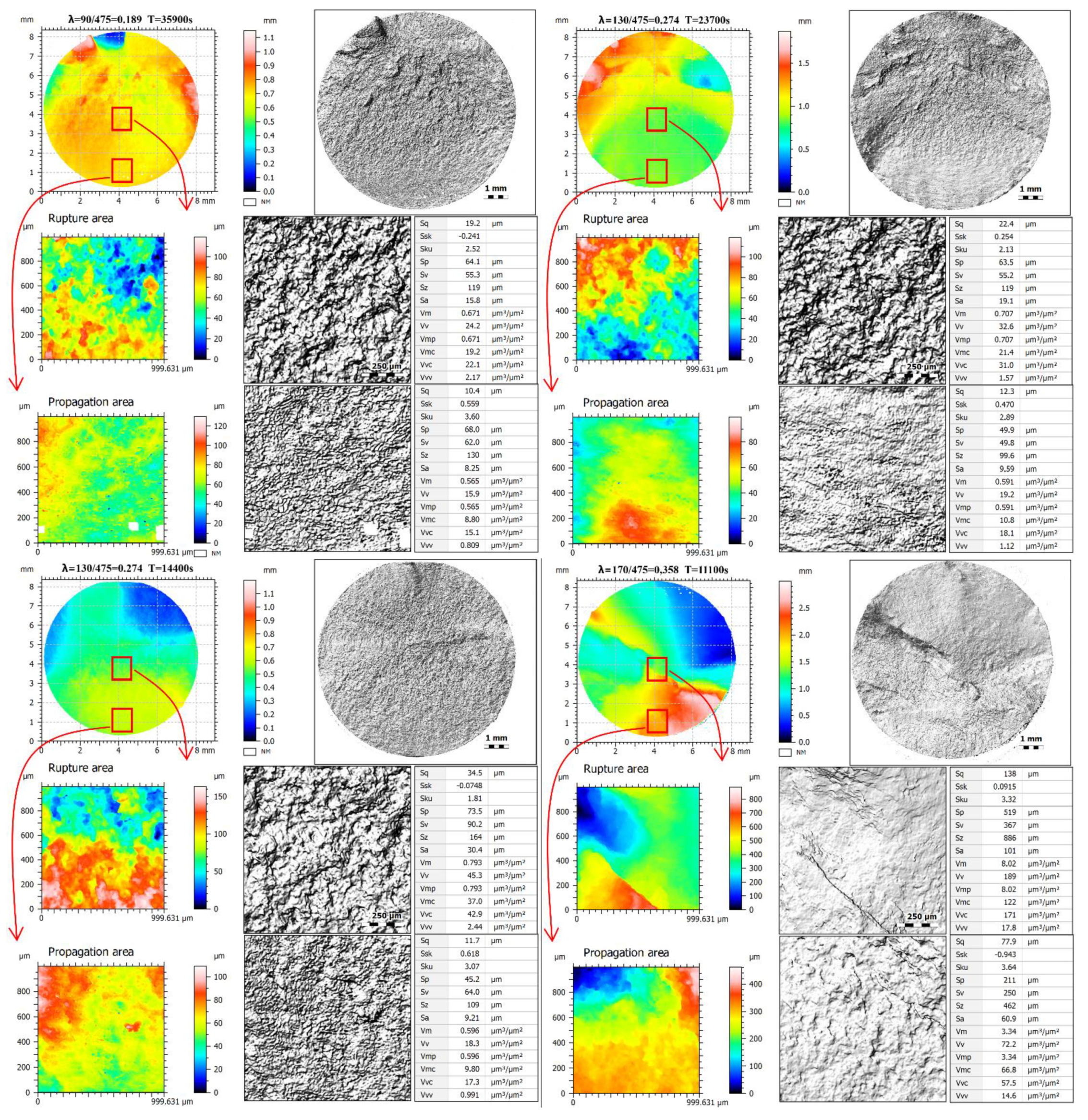
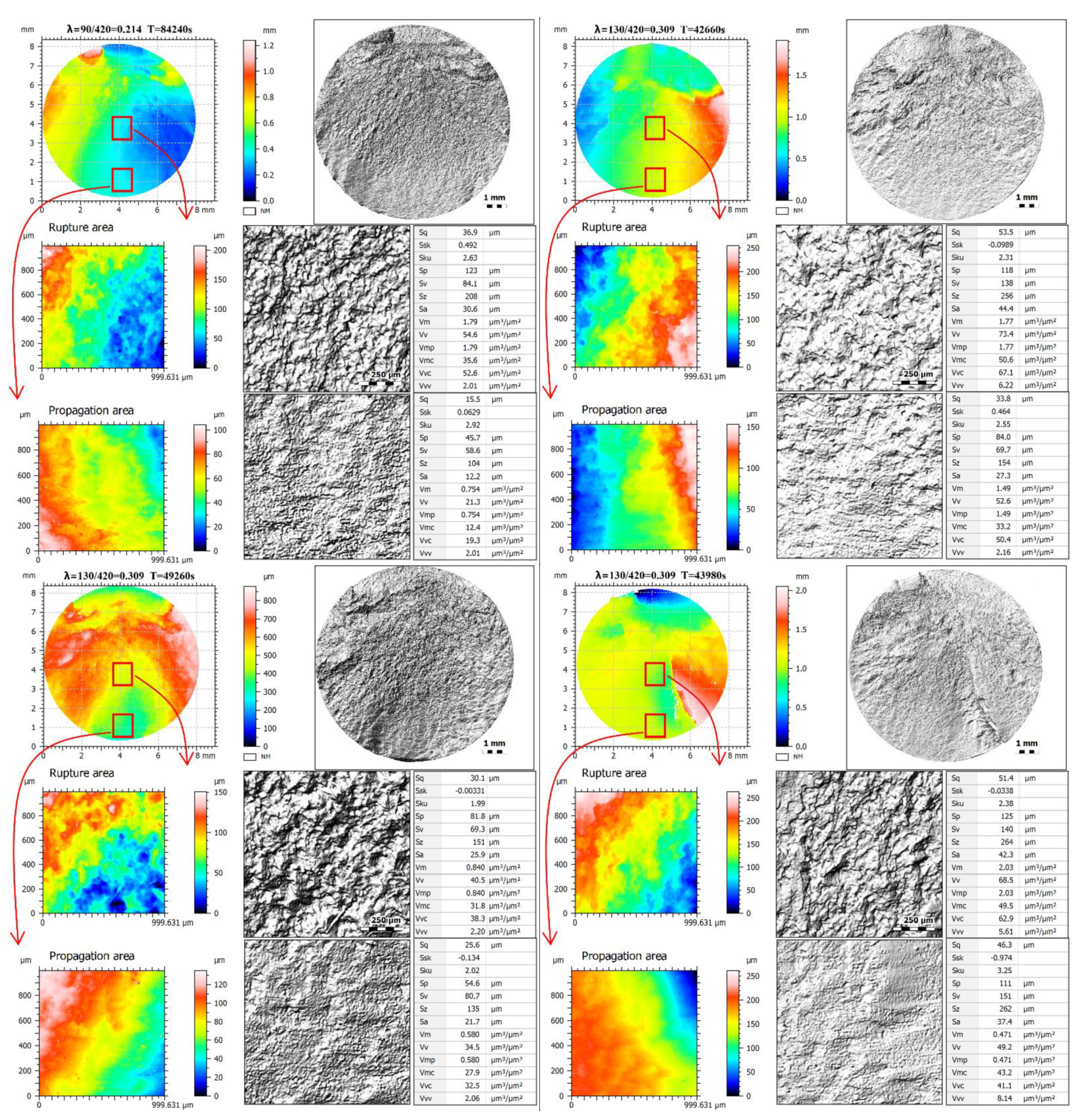
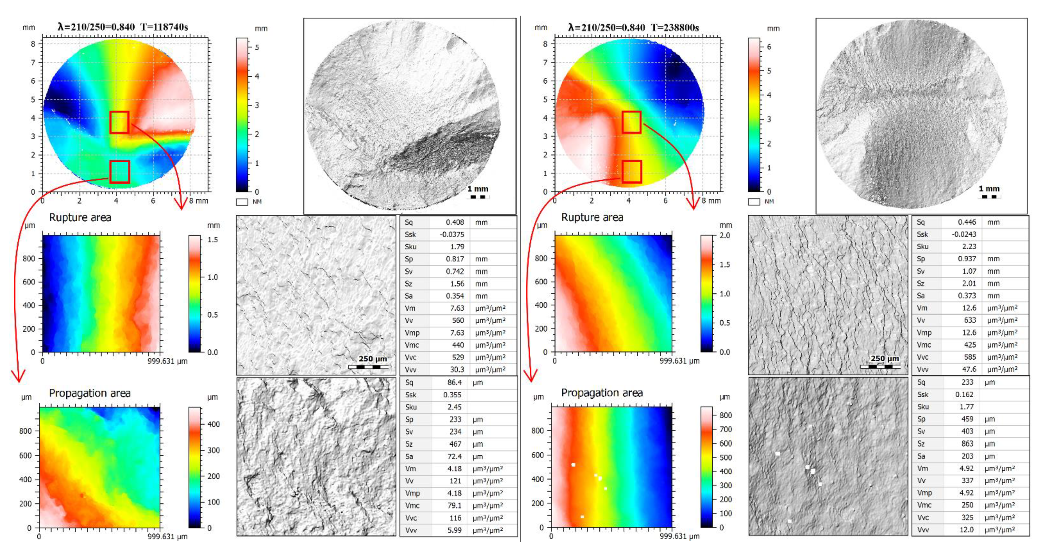
Regions of interest for (1) total (the whole current surface reduced to the circle with diameter 7.8 mm) [30], (2) propagation and (3) rupture areas are shown in Figure 4.
The fatigue fractures were investigated at the objective magnification of 10×. The main measurement parameters are summarized in Table 1. To realize total area scanning, the Imagefield function was used. The numbers of merged images were 9 rows and 7 columns.
Surface topography studies were carried out on the fracture area, using selected height parameter and functional (volume) parameters according to ISO 25178-2 [8,10], employing MountainsMap software. Sq (Equation (1)) is the root mean square height, while void volume Vv calculated for a material ratios Smr, by integrating the volume enclosed above the surface and below a horizontal cutting plane (Equation (2)). Graphical illustration of the functional (volume) parameters is presented in Figure 5.
S q = 1 A A z 2 ( x , y ) d x d y ,
where A is the definition area; z is the surface height in position x, y; x, y are the lengths in perpendicular directions.
V v ( S m r ) = k S m r 100 % [ h ( S m r ) h ( S m r x ) ] d S m r x ,
where h is a height; k is a factor to convert the volume into the required unit; for Smr = 100%, the Vv parameter is zero; for Smr = 0%, the void volume is a maximum (the cutting plane below the lowest point); for these cases, the areal material ratio Smr = Smr1 = 10% (see Figure 5).
Given the above definition (Equation (2)), core void volume Vvc and pit void volume Vvv can be represented by Equations (3) and (4), respectively.
Vvc = Vv(Smr1) − Vv(Smr2),
Vvv = Vv(Smr2).

3. Results

The results of bending-torsion fatigue test for S355J2 steel, shown in this section, was made with 11 different ratios of maximum stresses λ. The visualization of the individual three ROIs, together with the tables of surface topography measurements for the propagation and rupture areas, is shown in Figure 6. All 24 loading cases are presented in the order of reducing the maximum normal stress σmax value. Figure 6 also shows the results of the individual fatigue life T values.

4. Discussion

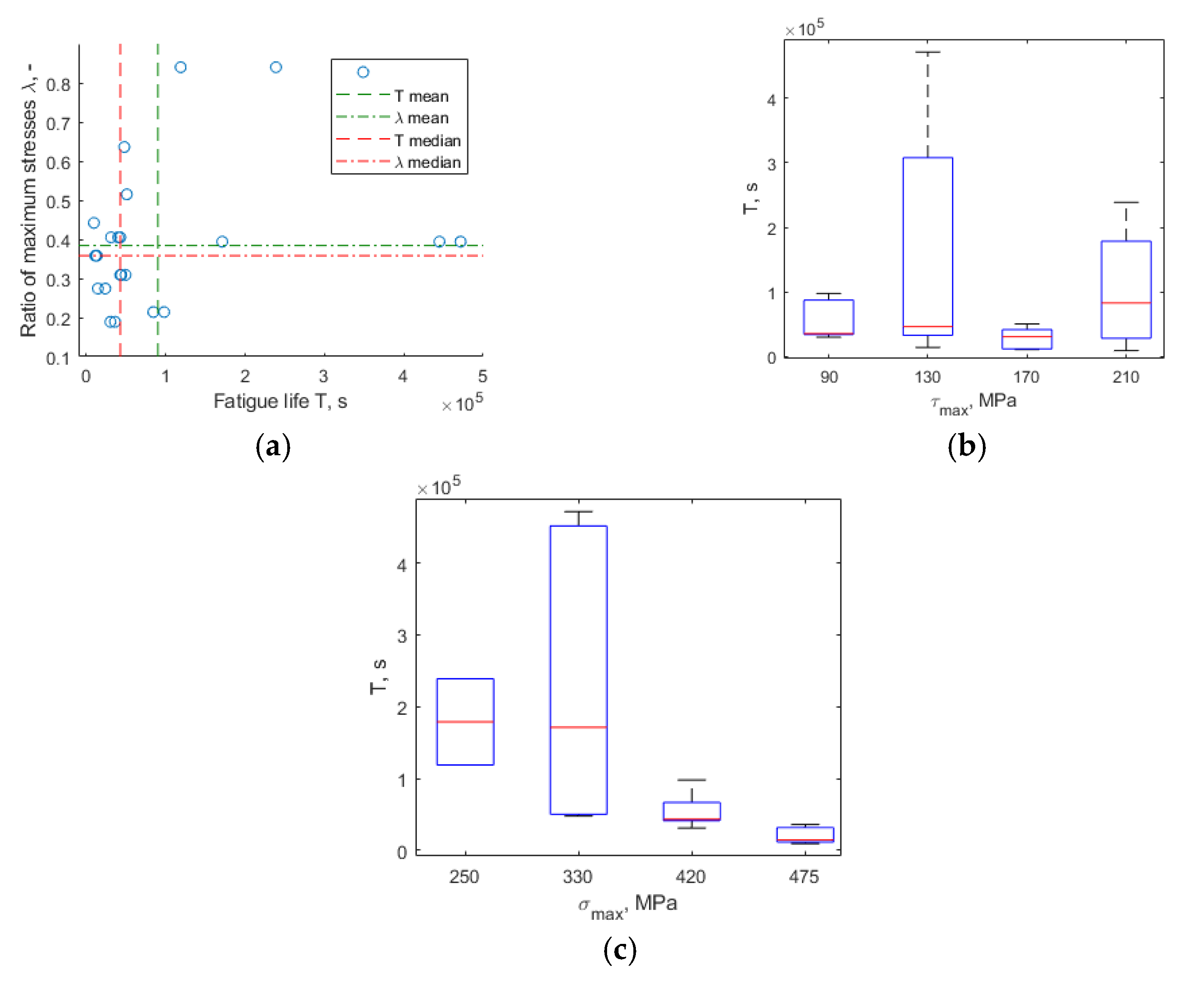
4.1. The Influence of the Maximum Normal and Shear Stresses Share on Fatigue Life

Figure 7a shows the results of fatigue life T in comparison with the ratio of maximum stresses λ. On the other hand, in Figure 7b,c there are boxplots with the shares of maximum shear stress τmax and maximum normal stress σmax, respectively.
From the plot in Figure 7a, it is possible to deduce a large dispersion of fatigue life T results depending on the ratio of maximum stresses λ. Therefore, in the further part of the work, the focus was on the selection of the most sensitive parameters of fracture surface topography to the ratio of maximum stresses λ. Figure 7b,c shows that fatigue life T depends more on the share of maximum normal stress σmax (see Figure 7c) than on the maximum shear stress τmax (see Figure 7b) in the applied fatigue loadings.

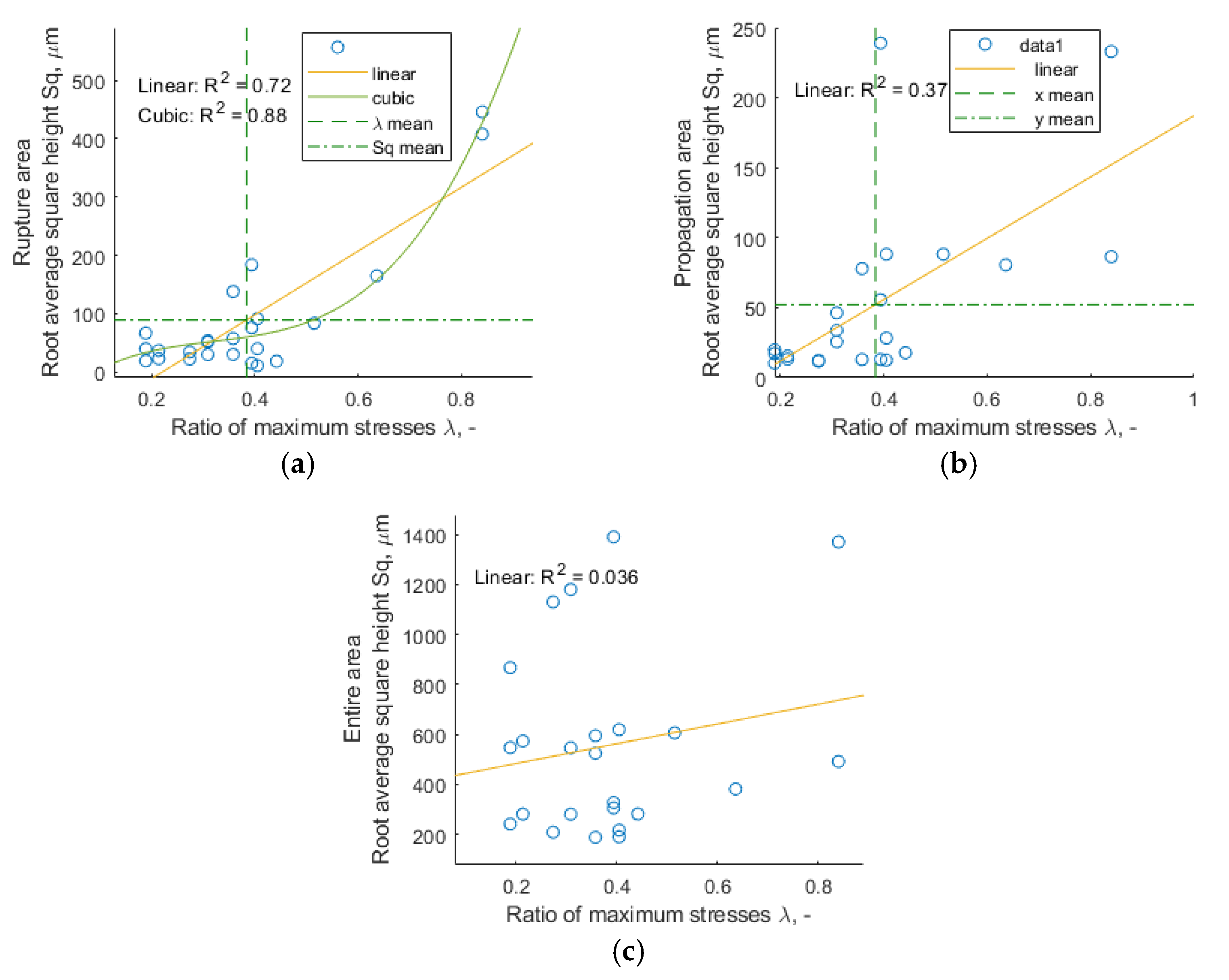
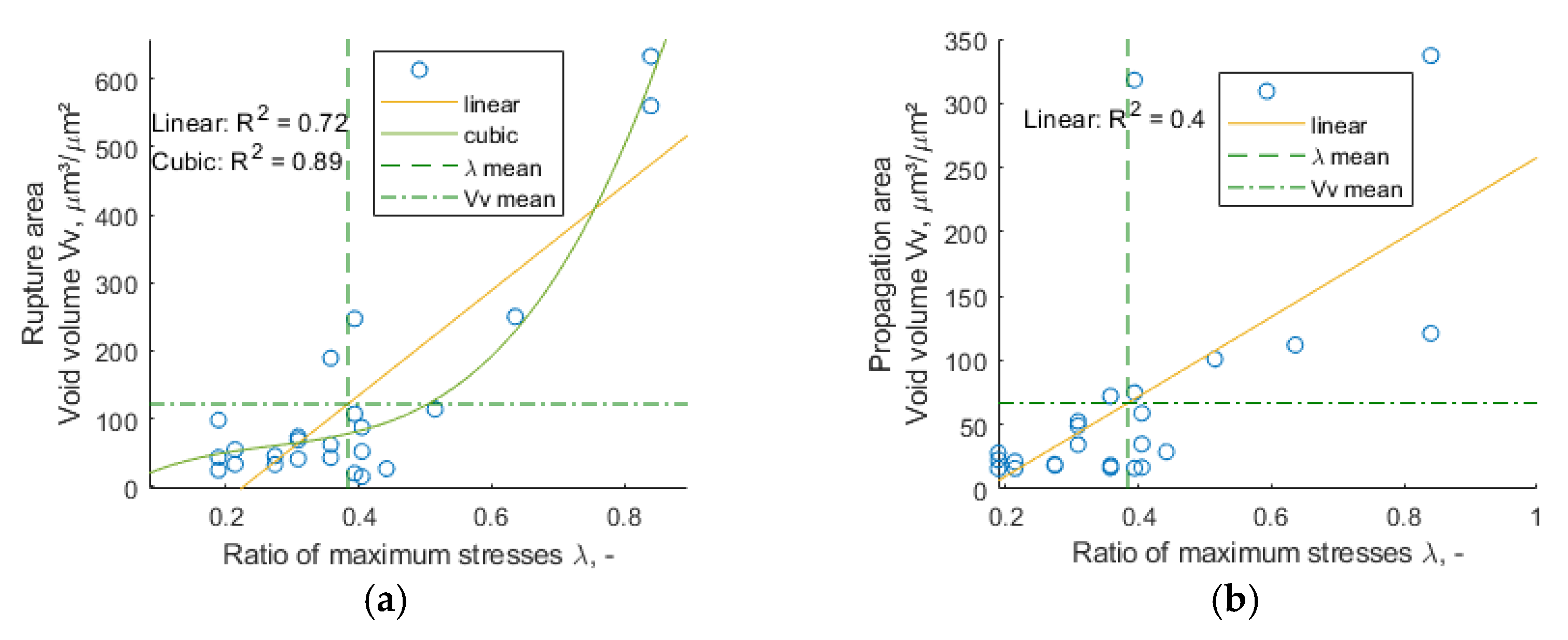
4.2. The Influence of the Ratio of Maximum Stresses λ on Fracture Surface Parameters

Figure 8 shows the ratio of maximum stresses λ vs. root mean square height Sq plots for rupture, propagation and entire fracture areas, respectively. Additionally, Figure 9 plots the λ ratio depending on the Vv parameter, in the same order of zones.
The best correlation with respect to ratio of maximum stresses λ was demonstrated by the void volume Vv parameter for the rupture area, for which the coefficient of determination R2 was 0.72 (linear fit). Therefore, for this case, looking for a better coefficient of determination, we found the one for cubic fitting, equal to R2 = 0.89. The best fit for the rupture zone may be due to the more stable results of the surface topography in that area. This, in turn, can be explained by not always matching propagation area and a greater range of surface topography changes near the edge of the specimen. The analyzed Vv parameter in the rupture area turned out to be better than in the entire fracture surface zone, which was taken into account in [30].
Figure 10 presents the relationship between the void volume Vv and the root mean square height Sq values for three analyzed zones.
Figure 10c confirms almost the same fit of root mean square height Sq to void volume Vv and the effectiveness of the measurements for the rupture zone.

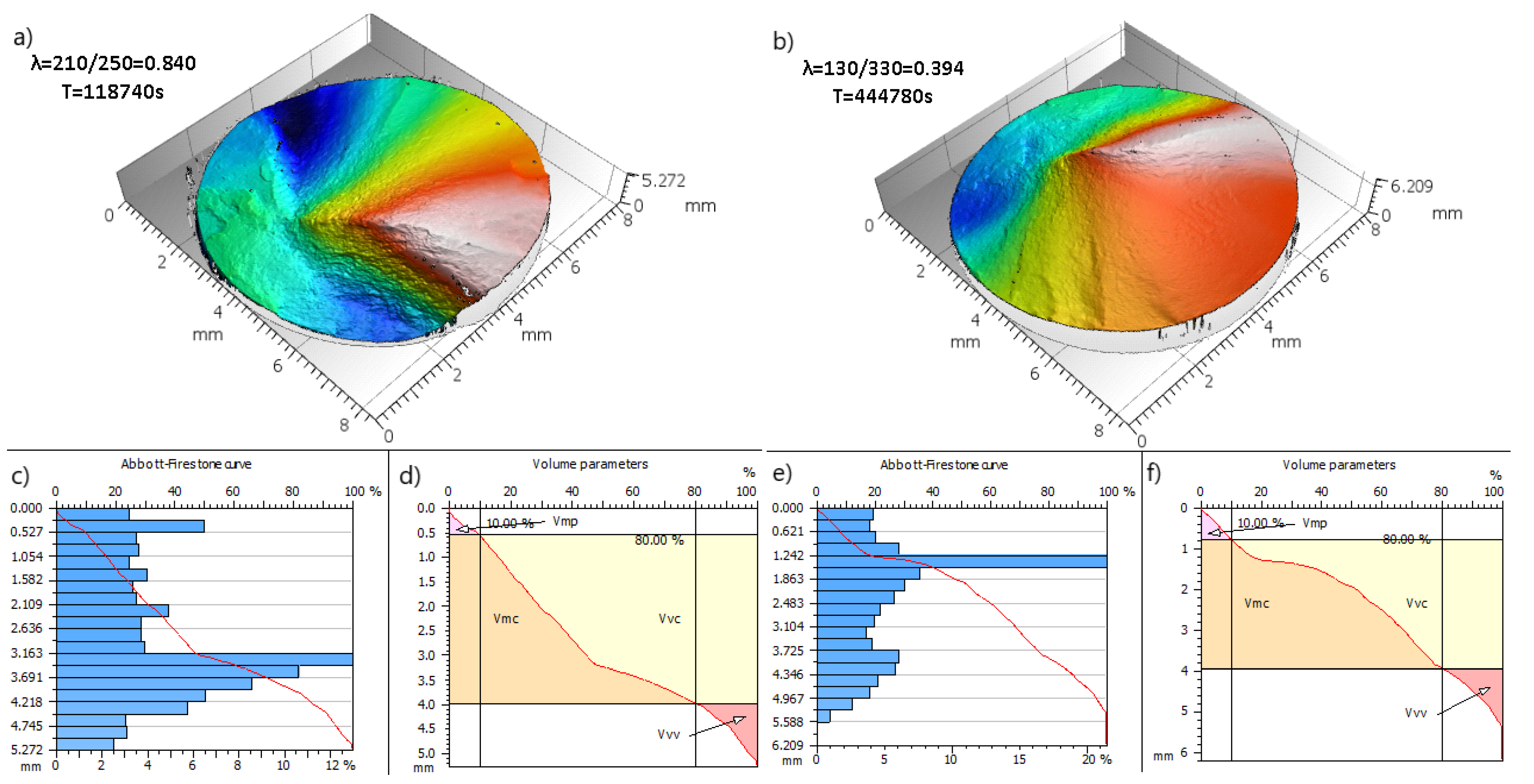
4.3. Fracture Surface Parameters for Maximum Vv Cases

The intentions of this subsection are to confront the standard surface parameters and their specified sensitivity to topology of fracture for extremal Vv surface parameter for the rupture zone. For this purpose, in addition to an isometric view of the fractures (see Figure 11a,b), the study of the Abbott–Firestone curve [34] is presented. Abbott–Firestone curves (see Figure 11c,e) are connected to the distribution of heights and its cumulated curve. Figure 11d,f shows the ISO 25178-2 functional volume parameters that are represented with respect to it: Vmp (peak material volume), Vmc (core material volume), Vvc (core void volume), Vvv (valley void volume), Vmp, Vmc, and Vvv sections, respectively. For these functional parameters, the areal material ratio Smr1 = 10% and Smr2 = 80% were specified [35].
The presented cases (see Figure 11), apart from the highest Vv values in the rupture area, are characterized by ones of the largest fatigue life T values. For the Abbott–Firestone plots (see Figure 11c,e), the maximum heights, in fractures surfaces of maximal Vv values for rupture area, demonstrate that the histogram distribution is slightly even. This is manifested by the fact that the largest measured height distribution takes a large value (about 13% and 21%). They have big values of height distribution due to extensive valleys. The maximum Vv values samples are characterized by wide Vmc and Vvc stripes (see Figure 11d,f), which proves the advantage of the core volume (material and void).

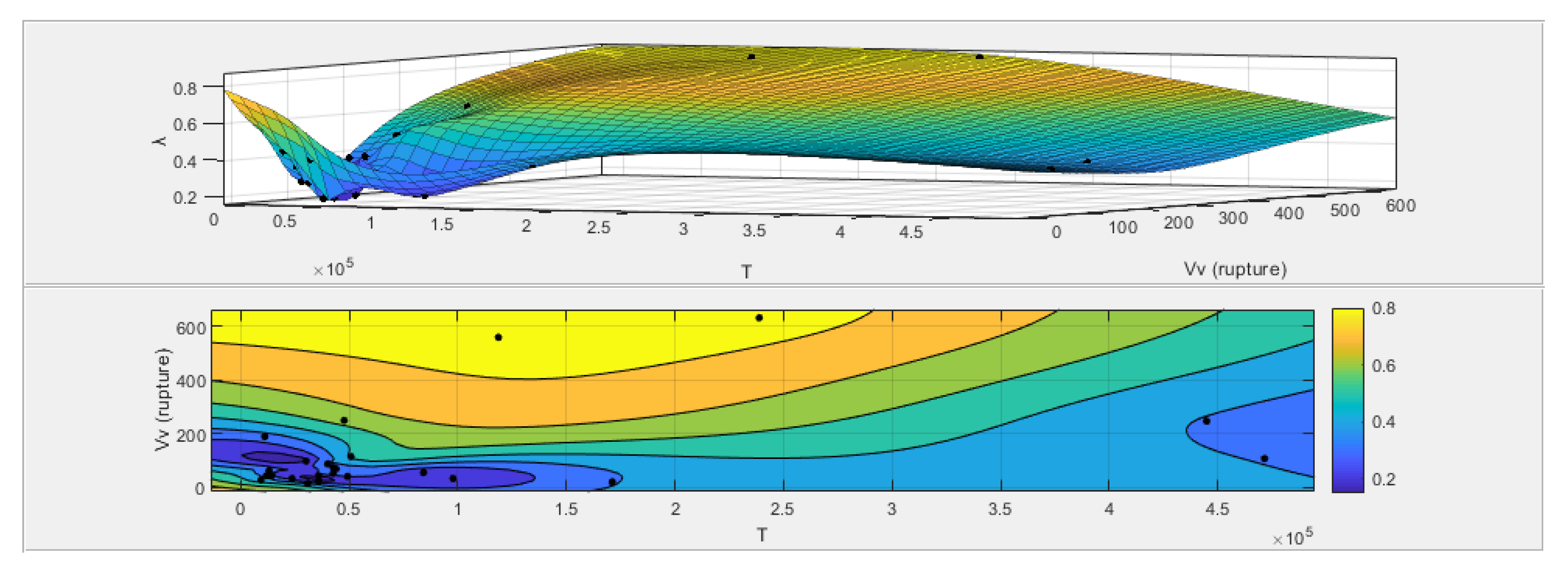
4.4. Summary of the Optimal Fractographic Parameter Vv with Fatigue Life T and Ratio of Maximum Stresses λ

Curve Fitting Toolbox in Matlab software provided a function for fitting curves and surfaces to data plotted in Figure 12 and Figure 13. Figure 12 shows the Gaussian fit and with residuals plots containing data from all 24 specimens analyzed, demonstrating the best correlation between Vv and T. Gaussian fitting coefficient of determination R2 took values of around 0.434, which along with other statistical parameters are presented in Table 2.
The thin-plate spline interpolant procedure was used to present the relation of void volume Vv, fatigue life T and ratio of maximum stresses λ (see Figure 13), assuming statistical coefficients, as in Table 3.

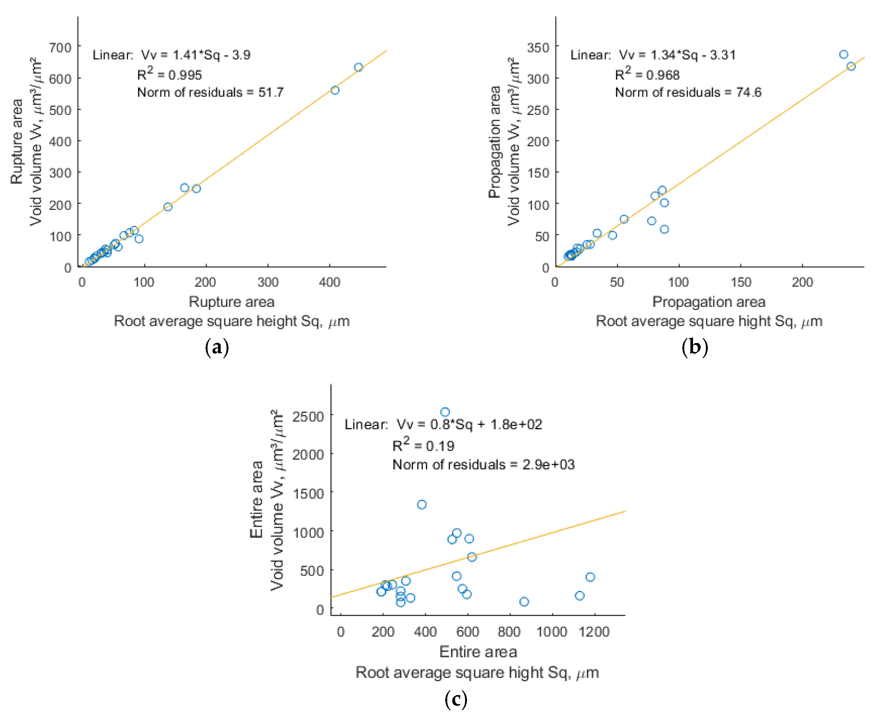
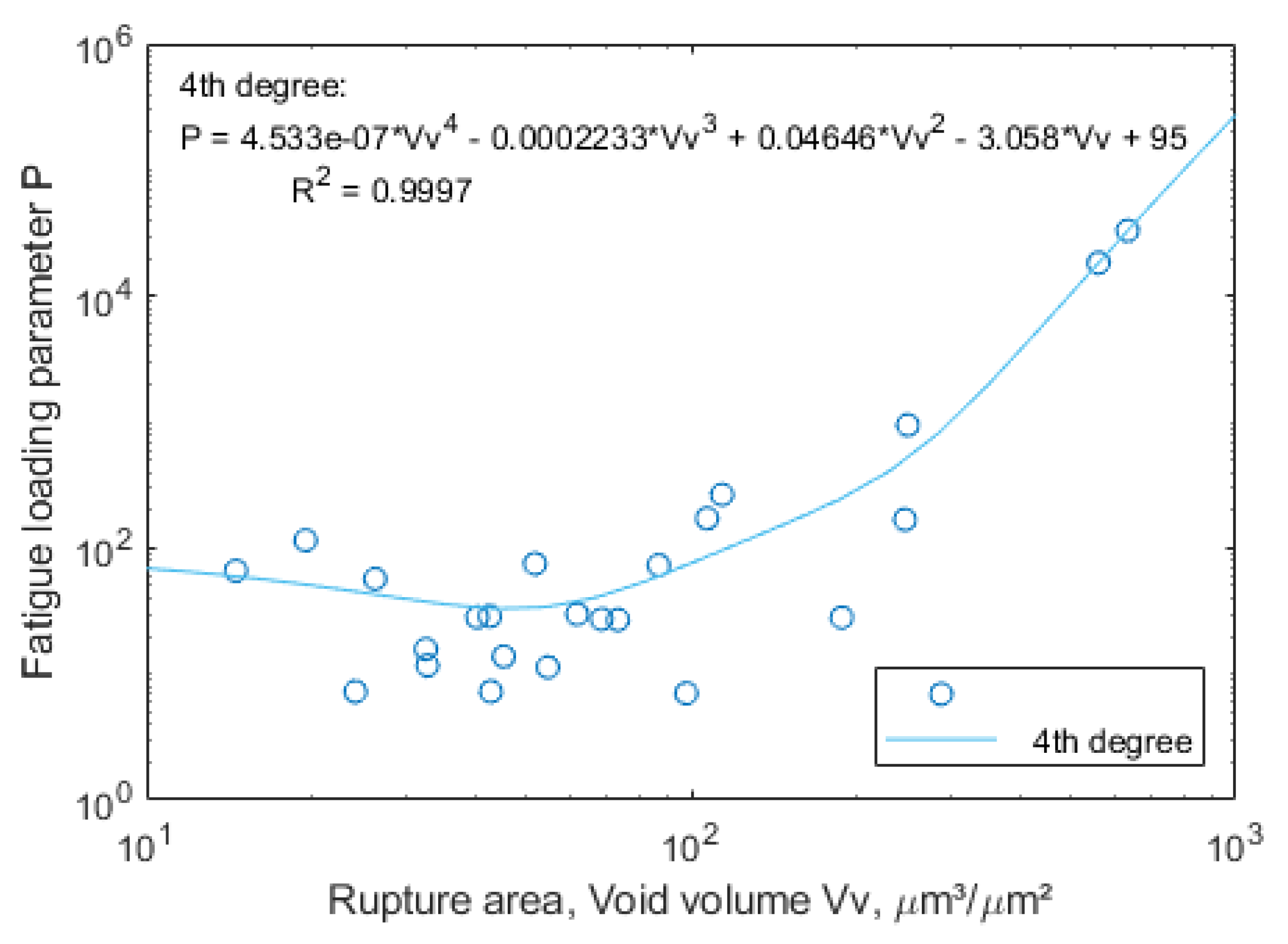
4.5. Loading and Fatigue Life Prediction Model Based on Void Volume Vv Parameter for the Rupture Area

To find closer relationships of the ratio of maximum stresses λ and fatigue life T, with the fracture surface topography, represented by void volume Vv in the rupture area, the new indicator called fatigue loading parameter P (Equation (5)) was proposed.
P = T λ ,
where: T is the fatigue life and λ is the ratio of maximum stresses (λ = τmaxmax).
The results of the fatigue loading parameter P vs. void volume Vv in the rupture area were plotted in log-log scale, see in Figure 14. Log-log(Vv, P) plots Vv- and P-coordinates using a base 10 logarithmic scale on the Vv-axis and the P-axis. Data points were subjected to the basic fitting tool, for which the 4th degree type of fit turned out to be the best fit, for which R2 = 0.9997. The presented model has some limitations, mainly related to the scope of the bending-torsion combination (λ).

5. Conclusions

In this paper the surface topography of fractures generated under pseudo-random non-proportional combined bending-torsion fatigue loading in three regions, (1) total, (2) propagation and (3) rupture, was studied. In total, 24 specimens made of S355J2 steel with 11 different ratio of maximum stresses λ were tested. The analyzed metrological parameters of the surface topography were root mean square height Sq and void volume Vv. The following conclusions are established:
  • Fatigue life T depends more on the share of maximum normal stress σmax than on the maximum shear stress τmax;
  • The best correlation with respect to ratio of maximum stresses λ was demonstrated by the void volume Vv parameter for the rupture area, and the best was Cubic fit with R2 around 0.89;
  • The loading factors also affect the shape of the Abbott–Firestone curve as well as the extent Vx volume parameters (Vmp, Vmc, Vvc and Vvv);
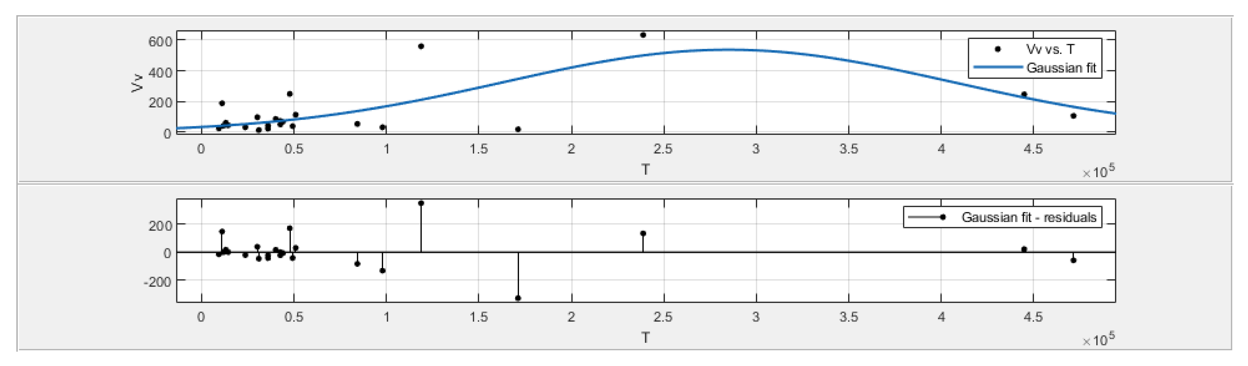
  • Fatigue life T, in the case of the analyzed data, is not well correlated with the surface topography parameters and the best was Gaussian fit with R2 around 0.434;
  • New fatigue loading parameter P shows a rather good fit to void volume Vv parameter for the rupture area, with R2=0.9997, but within the specified range of loading combinations.
Fracture measurements were performed using an Alicona G4 device, but the findings should be broadly applicable to any surface topography measuring instrument. The obtained results for the rupture area turned out to be more accurate than the Author’s best matched research using the entire fracture area method so far. From the point of view of methodology, such a solution is easier to implement and more universal. These methods should also be compared for other materials and loading types, in future investigations.

Funding

This research received no external funding.

Institutional Review Board Statement

Not applicable.

Informed Consent Statement

Not applicable.

Data Availability Statement

Not applicable.

Acknowledgments

The Author kindly acknowledges Zbigniew Marciniak, for sharing their specimens after fatigue test.

Conflicts of Interest

The authors declare no conflict of interest.

Nomenclature

hµmheight
P-fatigue loading parameter
R2-coefficient of determination
Saµmarithmetical mean height
Skµmcore height
Smr1, Smr2
Smr, Smrx%areal material ratio
Spkµmreduced peak height
Svkµmreduced dale height
Sqµmroot mean square height
Tsfatigue life
tstime
Vmcµm³/µm²core material volume
Vmpµm³/µm²peak material volume
Vvµm³/µm²void volume
Vvcµm³/µm²core void volume
Vvvµm³/µm²pit void volume
σ(t)MPanormal stress in time
τ(t)MPashear stress in time
σmaxMPamaximum normal stress
τmaxMPamaximum shear stress
λ-ratio of maximum stresses

References

  1. Branco, R.; Berto, F. High-Strength Low-Alloy Steels. Metals 2021, 11, 1000. [Google Scholar] [CrossRef]
  2. Guo, F.; Wu, S.C.; Liu, J.X.; Zhang, W.; Qin, Q.B.; Yao, Y. Fatigue life assessment of bogie frames in high-speed railway vehicles considering gear meshing. Int. J. Fatigue 2020, 132, 105353. [Google Scholar] [CrossRef]
  3. Cruces, A.S.; Lopez-Crespo, P.; Moreno, B.; Antunes, F.V. Multiaxial Fatigue Life Prediction on S355 Structural and Offshore Steel Using the SKS Critical Plane Model. Metals 2018, 8, 1060. [Google Scholar] [CrossRef] [Green Version]
  4. Pawliczek, R.; Rozumek, D. The Effect of Mean Load for S355J0 Steel with Increased Strength. Metals 2020, 10, 209. [Google Scholar] [CrossRef] [Green Version]
  5. Riofrío, P.G.; Ferreira, J.A.M.; Capela, C.A. Imperfections and Modelling of the Weld Bead Profile of Laser Butt Joints in HSLA Steel Thin Plate. Metals 2021, 11, 151. [Google Scholar] [CrossRef]
  6. Jiménez-Peña, C.; Goulas, C.; Preußner, J.; Debruyne, D. Failure Mechanisms of Mechanically and Thermally Produced Holes in High-Strength Low-Alloy Steel Plates Subjected to Fatigue Loading. Metals 2020, 10, 318. [Google Scholar] [CrossRef] [Green Version]
  7. Fu, S.; Cheng, F.; Tjahjowidodo, T. Surface Topography Measurement of Mirror-Finished Surfaces Using Fringe-Patterned Illumination. Metals 2020, 10, 69. [Google Scholar] [CrossRef] [Green Version]
  8. Podulka, P. The Effect of Surface Topography Feature Size Density and Distribution on the Results of a Data Processing and Parameters Calculation with a Comparison of Regular Methods. Materials 2021, 14, 4077. [Google Scholar] [CrossRef]
  9. Dzierwa, A.; Reizer, R.; Pawlus, P.; Grabon, W. Variability of areal surface topography parameters due to the change in surface orientation to measurement direction. Scanning 2014, 36, 170–183. [Google Scholar] [CrossRef]
  10. ISO-ISO 25178-2:2012—Geometrical Product Specifications (GPS)—Surface Texture: Areal—Part 2: Terms, Definitions and Surface Texture Parameters. Available online: https://www.iso.org/standard/42785.html (accessed on 28 December 2020).
  11. Todhunter, L.D.; Leach, R.K.; Lawes, S.D.A.; Blateyron, F. Industrial survey of ISO surface texture parameters. CIRP J. Manuf. Sci. Technol. 2017, 19, 84–92. [Google Scholar] [CrossRef]
  12. Zak, K. Cutting mechanics and surface finish for turning with differently shaped CBN tools. Arch. Mech. Eng. 2017, 64, 347–357. [Google Scholar] [CrossRef] [Green Version]
  13. Wojciechowski, S.; Maruda, R.W.; Barrans, S.; Nieslony, P.; Krolczyk, G.M. Optimisation of machining parameters during ball end milling of hardened steel with various surface inclinations. Measurement 2017, 111, 18–28. [Google Scholar] [CrossRef] [Green Version]
  14. Senin, N.; Thompson, A.; Leach, R.K. Characterisation of the topography of metal additive surface features with different measurement technologies. Meas. Sci. Technol. 2017. [Google Scholar] [CrossRef]
  15. Feng, X.; Senin, N.; Su, R.; Ramasamy, S.; Leach, R. Optical measurement of surface topographies with transparent coatings. Opt. Lasers Eng. 2019, 121, 261–270. [Google Scholar] [CrossRef]
  16. López-Sanz, S.; Guzmán Bernardo, F.J.; Rodríguez Martín-Doimeadios, R.C.; Ríos, Á. Analytical metrology for nanomaterials: Present achievements and future challenges. Anal. Chim. Acta 2019, 1059, 1–15. [Google Scholar] [CrossRef] [PubMed]
  17. Taylor, M.A.; Bowen, W.P. Quantum metrology and its application in biology. Phys. Rep. 2016, 615, 1–59. [Google Scholar] [CrossRef] [Green Version]
  18. Pluta, K.; Florkiewicz, W.; Malina, D.; Rudnicka, K.; Michlewska, S.; Królczyk, J.B.; Sobczak-Kupiec, A. Measurement methods for the mechanical testing and biocompatibility assessment of polymer-ceramic connective tissue replacements. Measurement 2021, 171, 108733. [Google Scholar] [CrossRef]
  19. Wu, Q.; Liu, X.; Liang, Z.; Wang, Y.; Wang, X. Fatigue life prediction model of metallic materials considering crack propagation and closure effect. J. Braz. Soc. Mech. Sci. Eng. 2020, 42, 1–11. [Google Scholar] [CrossRef]
  20. Derpeński, Ł.; Seweryn, A.; Bartoszewicz, J. Ductile fracture of notched aluminum alloy specimens under elevated temperature part 1—Experimental research. Theor. Appl. Fract. Mech. 2019, 102, 70–82. [Google Scholar] [CrossRef]
  21. Azevedo, C.R.F.; Marques, E.R. Three-dimensional analysis of fracture, corrosion and wear surfaces. Eng. Fail. Anal. 2010, 17, 286–300. [Google Scholar] [CrossRef]
  22. Lynch, S.P.; Moutsos, S. A brief history of fractography. J. Fail. Anal. Prev. 2006, 6, 54–69. [Google Scholar] [CrossRef]
  23. Hu, Y.; Wu, S.; Withers, P.J.; Cao, H.; Chen, P.; Zhang, Y.; Shen, Z.; Vojtek, T.; Hutař, P. Corrosion fatigue lifetime assessment of high-speed railway axle EA4T steel with artificial scratch. Eng. Fract. Mech. 2021, 245, 107588. [Google Scholar] [CrossRef]
  24. Macek, W.; Owsiński, R.; Trembacz, J.; Branco, R. Three-dimensional fractographic analysis of total fracture areas in 6082 aluminium alloy specimens under fatigue bending with controlled damage degree. Mech. Mater. 2020, 147, 103410. [Google Scholar] [CrossRef]
  25. Macek, W. Fractal analysis of the bending-torsion fatigue fracture of aluminium alloy. Eng. Fail. Anal. 2019, 99, 97–107. [Google Scholar] [CrossRef]
  26. Macek, W.; Branco, R.; Korpyś, M.; Łagoda, T. Fractal dimension for bending-torsion fatigue fracture characterisation. Measurement 2021, 184, 109910. [Google Scholar] [CrossRef]
  27. Macek, W.; Branco, R.; Costa, J.D.; Pereira, C. Strain sequence effect on fatigue life and fracture surface topography of 7075-T651 aluminium alloy. Mech. Mater. 2021, 160, 103972. [Google Scholar] [CrossRef]
  28. Macek, W.; Branco, R.; Szala, M.; Marciniak, Z.; Ulewicz, R.; Sczygiol, N.; Kardasz, P. Profile and Areal Surface Parameters for Fatigue Fracture Characterisation. Materials 2020, 13, 3691. [Google Scholar] [CrossRef]
  29. Macek, W. Fracture surface formation of notched 2017A-T4 aluminium alloy under bending fatigue. Int. J. Fract. 2021, 9, 1–17. [Google Scholar] [CrossRef]
  30. Macek, W.; Marciniak, Z.; Branco, R.; Rozumek, D.; Królczyk, G.M. A fractographic study exploring the fracture surface topography of S355J2 steel after pseudo-random bending-torsion fatigue tests. Measurement 2021, 178, 109443. [Google Scholar] [CrossRef]
  31. Marciniak, Z.; Rozumek, D.; Macha, E. Verification of fatigue critical plane position according to variance and damage accumulation methods under multiaxial loading. Int. J. Fatigue 2014, 58, 84–93. [Google Scholar] [CrossRef]
  32. Marciniak, Z.; Rozumek, D.; Macha, E. Fatigue lives of 18G2A and 10HNAP steels under variable amplitude and random non-proportional bending with torsion loading. Int. J. Fatigue 2008, 30, 800–813. [Google Scholar] [CrossRef]
  33. Macek, W.; Mucha, N. Evaluation of Fatigue Life Calculation Algorithm of the Multiaxial Stress-Based Concept Applied to S355 Steel under Bending and Torsion. Mech. Mech. Eng. 2017, 21, 935–951. [Google Scholar]
  34. Abbott, E.J.; Firestone, F.A. Specifying surface quality. Mech. Eng. 1933, 65, 569–572. [Google Scholar]
  35. Pawlus, P.; Reizer, R.; Wieczorowski, M.; Krolczyk, G. Material ratio curve as information on the state of surface topography—A review. Precis. Eng. 2020, 65, 240–258. [Google Scholar] [CrossRef]
Figure 1. The real S355J2 steel specimen after fatigue test.
Metals 11 01620 g001
Figure 2. Pseudorandom stress histories in time: (a) normal stress σ(t); and (b) shear stress τ(t). Adopted from [33].
Metals 11 01620 g002
Figure 3. Maximum normal stress σmax and maximum shear stress τmax, grouped by fatigue life T.
Metals 11 01620 g003
Figure 4. Extracting methodology used to fit the region of interest (ROI).
Metals 11 01620 g004
Figure 5. Graphical presentation of the functional (volume) parameters: (a) an exemplary surface profile; (b) functional (volume) parameters of Abbott–Firestone curve according to ISO 25178.
Metals 11 01620 g005
Figure 6. Visualization at different applied ratios of maximum stresses λ for the investigated ROIs: (1) total; (2) propagation; (3) rupture.
Metals 11 01620 g006aMetals 11 01620 g006bMetals 11 01620 g006cMetals 11 01620 g006dMetals 11 01620 g006eMetals 11 01620 g006fMetals 11 01620 g006g
Figure 7. Fatigue life T in context: (a) ratio of maximum stresses λ; (b) maximum shear stress τmax; (c) maximum normal stress σmax.
Metals 11 01620 g007
Figure 8. Areal surface parameter Sq evaluation at different applied ratio of maximum stresses λ for the investigated zones: (a) rupture area; (b) propagation area; (c) entire area.
Metals 11 01620 g008
Figure 9. Void volume Vv evaluation at different applied ratios of maximum stresses λ for the investigated zones: (a) rupture area; (b) propagation area; (c) entire area.
Metals 11 01620 g009aMetals 11 01620 g009b
Figure 10. Relationship between void volume Vv and Sq parameter values: (a) rupture area; (b) propagation area; (c) entire area.
Metals 11 01620 g010
Figure 11. Fractures maximal Vv values for rupture area: (a,b) an isometric view of the entire fractures; (c,e) Abbott–Firestone curves; and (d,f) functional volume parameters plots.
Metals 11 01620 g011
Figure 12. Gaussian Vv vs. T curve fitting with residuals.
Metals 11 01620 g012
Figure 13. Relationship between Vv, T and λ values.
Metals 11 01620 g013
Figure 14. Fatigue loading parameter P vs. void volume Vv in the rupture area and their 4th degree fit.
Metals 11 01620 g014
Table 1. Alicona G4 measurement device main parameters.
Magnification10×
Vertical resolution79.6 nm
Lateral resolution3.91 µm
Number of images9 rows × 7 columns
Exposure time178 µs
Contrast0.53
Table 2. Gaussian curve fitting model parameters for Vv vs. T.
Curve Fitting, General Model Gauss1Goodness of Fit
f(x) = a1 × exp(−((x − b1)/c1)^2)SSE: 3.351 × 10⁵
Coefficients (with 95% confidence bounds):R2: 0.4336
a1 = 537.1 (280, 794.2)Adjusted R2: 0.3797
b1 = 2.848 × 10⁵ (2.379 × 10⁵, 3.316 × 10⁵)RMSE: 126.3
c1 = 1.721 × 10⁵ (1.242 × 10⁵, 2.2 × 10⁵)
Table 3. Gaussian curve fitting model parameters for Vv, T vs. λ.
Thin-Plate Spline InterpolantGoodness of Fit
f(x,y) = thin-plate spline computed from pp = coefficient structure
x is normalized by mean 9.003 × 10⁴ and std 1.256 × 10⁵SSE: 7.196 × 10⁻²⁶
y is normalized by mean 121.5 and std 160.4R2: 1
Publisher’s Note: MDPI stays neutral with regard to jurisdictional claims in published maps and institutional affiliations.

