Article

Researching a Moving Target Detection Method Based on Magnetic Flux Induction Technology

1
Beijing Institute of Spacecraft Environment Engineering, Beijing 100094, China
2
College of Electronic and Information, Southwest Minzu University, Chengdu 610041, China
3
Institute of Remote Sensing Satellite, CAST, Beijing 100094, China
*
Authors to whom correspondence should be addressed.
Metals 2021, 11(12), 1967; https://doi.org/10.3390/met11121967
Submission received: 16 August 2021 / Revised: 10 November 2021 / Accepted: 14 November 2021 / Published: 7 December 2021
(This article belongs to the Special Issue Advances in Metal-Containing Magnetic Materials)

Abstract

:
The ocean is a very important arena in modern warfare where all marine powers deploy their military forces. Due to the complex environment of the ocean, underwater equipment has become a very threatening means of surprise attack in modern warfare. Therefore, the timely and effective detection of underwater moving targets is the key to obtaining warfare advantages and has important strategic significance for national security. In this paper, magnetic flux induction technology was studied with regard to the difficulty of detecting underwater concealed moving targets. Firstly, the characteristics of a magnetic target were analyzed and an equivalent magnetic dipole model was established. Secondly, the structure of the rectangular induction coil was designed according to the model, and the relationship between the target’s magnetism and the detection signal was deduced. The variation curves of the magnetic flux and the electromotive force induced in the coil were calculated by using the numerical simulation method, and the effects of the different motion parameters of the magnetic dipole and the size parameters of the coil on the induced electromotive force were analyzed. Finally, combined with the wavelet threshold filter, a series of field tests were carried out using ships of different materials in shallow water in order to verify the moving target detection method based on magnetic flux induction technology. The results showed that this method has an obvious response to moving targets and can effectively capture target signals, which verifies the feasibility of the magnetic flux induction detection technology.

1. Introduction

The ocean is a very important stage in modern warfare where all countries deploy various military forces [1,2]. With the development of science and technology, modern marine warfare not only involves the competition of various advanced technologies, such as electronic and information technologies, but has also evolved into multiple space dimensions, including confrontations under water, on the sea’s surface, in the air, and even in space [3]. Among these, various types of underwater moving targets play important roles. Underwater moving targets, which are shielded by the vast ocean, are the most concealed equipment in the modern naval equipment system. Since the Second World War, the research into and development of technology for detecting underwater moving targets has progressed rapidly, especially regarding the application of nuclear technology, which makes underwater equipment a very threatening means of surprise attack in modern warfare. Various countries around the world, especially maritime powers, are currently developing and deploying different types of underwater targets. In modern marine warfare, the key to obtaining a warfare advantage is to find underwater moving targets in a timely and effective manner.
In the development of underwater moving target detection technology, optical, electrical, thermal, and other technical means have been applied [4,5,6,7,8,9,10,11,12]. Among these, the acoustic signal detection of underwater man-made objects has become the most widely used detection method. Sonar technology [13,14,15] was the first mature technology to be applied to underwater detection. It uses the propagation characteristics of sound waves in water to complete the task of detecting large underwater targets through electroacoustic conversion and signal processing. However, sonar detection has inherent disadvantages. It is easy for active sonar to expose its own position to the enemy, which has become its fatal disadvantage. Passive sonar detects the target only when it emits a relatively large noise. Due to the complex marine environment, the accuracy of the target resolution of sonar detection is limited. In addition, sonar detection has its own limitations, such as “sound shadow area”. With the rapid development and application of stealth technology, low noise and high acoustic stealth have evolved into revolutionary metrics in underwater moving target design. According to the data, the noise caused by the new underwater moving targets that have been continuously launched by the United States, Russia, and other countries in recent years has been lower than that of the marine background environment, meaning that it is difficult to find, identify, and track them by sonar. Therefore, there is an urgent need for new underwater moving target detection methods to make up for the shortcomings of the existing detection technologies.
Based on the principle of magnetic flux induction technology, this paper proposes a passive method that can be used to obtain and analyze the change in magnetic flux signal caused by underwater moving targets. According to the characteristics of moving targets, a magnetic dipole model [16,17,18,19] is established, the expressions of the magnetic flux of moving targets passing through a rectangular coil and the change in the electromotive force induced in the coil are deduced and calculated, and the influence of the various characteristic parameters on the induced electromotive force is analyzed. Finally, characteristic parameters such as the speed, depth, and magnetic moment of the targets can be obtained. This method has the advantages of a short execution time, lower impact from the complex shallow sea environment, all-weather working ability, and low cost. It is of great significance for providing early warnings of moving targets in coastal water areas, for island defense, and for providing early warnings in key areas.

2. Methods

When a moving target is close to a detection coil, the magnetic field of this target can be simulated by multiple magnetic dipoles; when the distance is far—that is, when the distance is greater than 3 times the size of the target—it can be treated as one magnetic dipole. This paper mainly focuses on the long-distance situation, so the magnetic field of a moving target can be simplified into one magnetic dipole model. The following is our research on the response relationship between the detection signal and the characteristics of the moving target based on this model.

2.1. Magnetic Flux Density of the Magnetic Dipole at Any Point in Space

In order to quantitatively analyze the change in electromotive force induced in a magnetic moving target in a detection closed coil, the magnetic dipole was simplified as a circular current and its coordinate system was established. As shown in Figure 1, the origin O of the coordinate system is located in the center of the magnetic dipole, the z-axis points in the direction of the magnetic moment vector, and the x-axis and y-axis point in accordance with the right-hand rule. E is a point in space whose spherical coordinate is E( r , φ 0 , θ 0 ).
Let the intensity of the circular current be I with unit A. The radius of a circle is R with unit m and r is the distance from the center O to a point in space with unit m. According to the Biot–Savart law [20] and the concept of magnetic moment [21], the following equations can be obtained:
{ B x = 3 μ 8 π p m ( R 2 + r 2 ) 3 r 2 sin 2 φ 0 cos θ 0 ( R 2 + r 2 ) B y = 3 μ 8 π p m ( R 2 + r 2 ) 3 r 2 sin 2 φ 0 sin θ 0 ( R 2 + r 2 ) B z = μ 2 π p m ( R 2 + r 2 ) 3 ( 1 3 2 r 2 sin 2 φ 0 R 2 + r 2 )
This is a set of expressions of the magnetic flux density of the space point E(r, φ 0 , θ 0 ) in three directions. For the far field—i.e., R < < r —expressions can be simplified by eliminating R. The x and y components of the magnetic flux density at any point in space are related to pm, r, φ 0 , and θ 0 , while the z component is only related to pm, r, φ 0 , and θ 0 .

2.2. Expression Derivation of Magnetic Flux in the Rectangular Coil at a Certain Time

For a rectangular detection coil with length a and width b whose number of turns is N, a rectangular coordinate system is established with the center of the coil as the zero point, as shown in Figure 2. The point Q(xq, 0, zq) in the figure is the moving target with the magnetic moment m. The target Q passes along the positive direction of the x-axis at a uniform speed v directly above the coil. P(xP, yP, 0) represents any point within the rectangular coil. Since this paper focuses on the long-distance situation—that is, R < < r —the magnetic flux density of the magnetic dipole Q at point P can be calculated using Equation (1). Since the magnetic flux passing through the rectangular coil is only related to the magnetic flux density perpendicular to the plane where the rectangular coil is located, it can be divided into three cases according to the different magnetic moment directions of the magnetic dipole.

2.2.1. The Direction of Magnetic Moment in Positive X Direction

According to the coordinate transformation relationship, the magnetic flux in the rectangular coil was related to B x in the magnetic dipole coordinate system shown in Figure 2, where R = 0, r = ( x p x q ) 2 + y p 2 + z q 2 . The following expression could be obtained by substituting R and r into Equation (1):
B x = 3 μ m 8 π 1 [ ( x p x q ) 2 + y p 2 + z q 2 ] 3 sin 2 φ cos θ
where:
sin φ = y p 2 + z q 2 ( x p x q ) 2 + y p 2 + z q 2
cos θ = z q y p 2 + z q 2
The magnetic flux through the rectangular coil can be obtained as follows:
Φ = a 2 a 2 b 2 b 2 B z d x d y = 3 μ m 4 π - a 2 a 2 - b 2 b 2 [ ( x x q ) 2 + y 2 + z q 2 ] 5 2 ( x x q ) z q d x d y
The above equation shows the magnetic flux generated in the rectangular coil by the magnetic dipole whose magnetic moment is in the positive x direction.

2.2.2. The Magnetic Moment in Positive Y Direction

According to the coordinate transformation relationship, the magnetic flux in the rectangular coil is related to B y in the magnetic dipole coordinate system shown in Figure 2:
B y = 3 μ m 8 π 1 [ ( x p x q ) 2 + y p 2 + z q 2 ] 3 sin 2 φ sin θ
where:
sin φ = ( x p x q ) 2 + z q 2 ( x p x q ) 2 + y p 2 + z q 2
cos φ = y p ( x p x q ) 2 + y p 2 + z q 2
sin θ = z q ( x p x q ) 2 + z q 2
The magnetic flux through the rectangular coil can be obtained as follows:
Φ = a 2 a 2 b 2 b 2 B z d x d y = 3 μ m 4 π - a 2 a 2 - b 2 b 2 B y d x d y = 0
It can be seen that when the magnetic moment of the magnetic dipole is in the positive y direction, the magnetic flux generated in the rectangular coil is zero.

2.2.3. The Magnetic Moment in Positive Z Direction

According to the coordinate transformation relationship, the magnetic flux in the rectangular coil is related to B z in the magnetic dipole coordinate system shown in Figure 2:
B z = μ m 2 π 1 [ ( x p x q ) 2 + y p 2 + z q 2 ] 3 ( 1 3 2 sin 2 φ )
where:
sin φ = ( x p x q ) 2 + y p 2 ( x p x q ) 2 + y p 2 + z q 2
The magnetic flux through the rectangular coil can be calculated using the following equation:
Φ = a 2 a 2 b 2 b 2 B z d x d y = a 2 a 2 b 2 b 2 μ m 2 π 1 [ ( x x q ) 2 + y 2 + z q 2 ] 3 ( 1 3 2 ( ( x x q ) 2 + y 2 ( x x q ) 2 + y 2 + z q 2 ) 2 ) d x d y = μ m 4 π - a 2 a 2 - b 2 b 2 [ ( x x q ) 2 + y 2 + z q 2 ] - 5 2 [ - ( x x q ) 2 y 2 + 2 z q 2 ] d x d y
The above equation is the magnetic flux generated in the rectangular coil by the magnetic dipole whose magnetic moment is in the positive z direction.
According to Faraday’s law of electromagnetic induction, the induced electromotive force at time t can be obtained by differentiating the magnetic flux ε = n Δ ϕ Δ t with respect to time t, where n is the number of coil turns.

3. Simulation Calculation

3.1. Influence of the Target’s Magnetic Moment Direction on Induced Electromotive Force

Suppose a magnetic dipole with a magnetic moment of 50 А·m2 whose height from the coil is h = 20 m is initially located at −100 m. This magnetic dipole moves along the x-axis with a dynamic speed of v = 1 m/s for 200 s. The coil has a length of a = 20 m and a width of b = 5 m, with a number of turns N = 100 and a magnetic permeability of μ = 4π × 10−7 H/m.
When the magnetic moment of the magnetic dipole is in the positive x direction, the simulation results are as shown in the figures below.
It can be seen from Figure 3 that for the magnetic moment of the magnetic dipole pointing in the positive x direction, the magnetic flux generated in the rectangular coil first increases from zero and then decreases back to zero when the magnetic dipole is right below the coil at 100 s. After that, it again increases and then decreases to zero in the opposite direction. The induced electromotive force first increases in the opposite direction from zero to a negative value, then increases in the positive direction, reaching the maximum when the dipole is right below the coil at 100 s. After that, it decreases back to a negative value and finally returns to zero.
When the magnetic moment of the magnetic dipole is in the positive z direction, the simulation results are as shown in the figures below.
It can be seen from Figure 4 that for the magnetic moment of the magnetic dipole pointing in the positive z direction, the magnetic flux generated in the rectangular coil first increases a small amount from zero in the positive direction, then increases continuously in the opposite direction, reaching the maximum when the magnetic dipole is right below the coil at 100 s. After that, it decreases to a certain positive value and finally returns to zero. The induced electromotive force first increases from zero and then decreases back to zero when the magnetic dipole is right below the coil at 100 s. After that, it again increases and then decreases to zero in the opposite direction. For a magnetic dipole whose magnetic moment is in an arbitrary direction, when calculating the induced electromotive force its magnetic moment should be decomposed along the coordinate axes. Calculations should be carried out separately and the overall induced electromotive force should be superimposed.

3.2. Influence of the Target’s Motion Parameters on Induced Electromotive Force

In this section, two parameters, the height h of the magnetic dipole from the coil and its moving speed v, were selected in order to analyze their influence on the induced electromotive force. For simplification, the magnetic moment of the magnetic dipole was set to pointing in the positive x direction.
In four different simulation cases, the height was set to zq = 20 m, zq = 25 m, zq = 30 m, and zq = 35 m, respectively, and other parameters were kept the same as those in Section 3.1.
Figure 5 shows the influence of the magnetic dipole’s height on the induced electromotive force. It can be seen that the induced absolute value of the electromotive force decreases with the increase in height h. There is a power exponential relationship between the peak value of the induced electromotive force and the height, and the index is related to the coil size.
Then, in four other simulation cases, the speed is set to v = 2 m/s, v = 1.5 m/s, v = 1 m/s, v = 0.5 m/s, and v = 0.25 m/s for the simulation calculations, and the other parameters arere the same as those in Section 3.1.
Figure 6 shows the influence of velocity on the induced electromotive force. It can be seen that the absolute value of the induced electromotive force increases with the increase in speed v. There is a linear relationship between the peak value of the induced electromotive force and the speed.

3.3. Influence of the Coil’s Size Parameters on Induced Electromotive Force

According to our theoretical analysis, when the coil size and the height h from the magnetic dipole to the coil were of the same order of magnitude, the larger the coil size, the greater the induced electromotive force. Due to the complex influence situation, only two cases with coil sizes of a = 20 m, b = 5 m, and a = 20 m, b = 30 m were subjected to a comparative analysis. Other parameters were the same as those in Section 3.1.
As can be seen from Figure 7, in a certain range, when the coil size was increased, the induced electromotive force also increased to a certain extent. Through further analysis, it could be concluded that the coil size would affect the power exponential relationship between the peak value of the induced electromotive force and the magnetic dipole height h. The larger the coil size, the smaller the exponential index.

4. Test Verification

After a field investigation, the research group selected a coastal area to carry out a series of field tests on the sea. In the test process, targets with different magnetic characteristics passed through the detection coil many times, and the obtained target magnetic flux signal was processed and analyzed by the wavelet threshold filtering method [22,23,24,25] to extract the required information.

4.1. The Detection Coil

The detection coil and data acquisition equipment used in the trials are shown in Figure 8. The coil wound by copper wire had a thickness of 10 cm, a frame size of 100 cm × 150 cm, and 500 turns. The copper wire diameter was 0.7 mm and the length of the conductive cable was about 150 m. An eight-channel data acquisition system with 128 Gb of memory was adopted. The coil was put into the sea at a depth of 10 m. Various types of ships passed over the coil many times at different speeds and from different distances so as to obtain the target flux signals under different motion states.

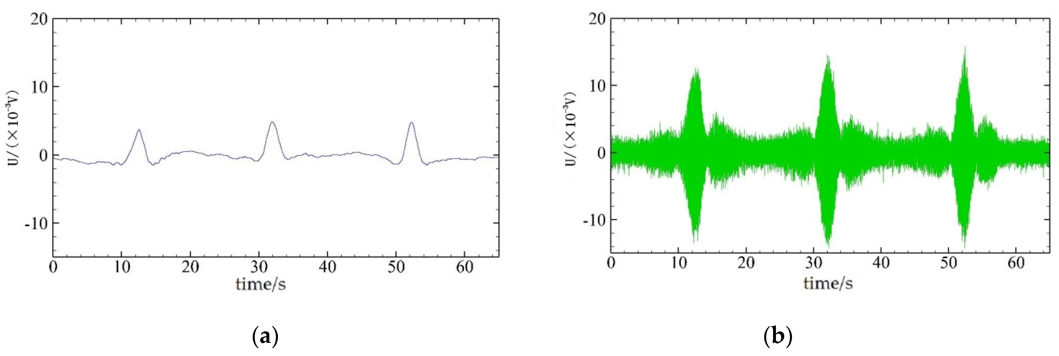
4.2. Result Analysis of the Extracted Magnetic Flux Signals of the Wooden Ship

As shown in Figure 9, a wooden ship passed over the detection coil in the field tests.
It can be seen from the figure that the curve of the target magnetic flux signal fluctuated obviously, but some local features were covered by the background noise. The wavelet threshold filtering method was used to process the magnetic flux signal. The low-frequency part and the high-frequency part after thresholding were reconstructed separately. The results are shown in Figure 10.
After analysis, it could be concluded that the low-frequency part of the magnetic flux signal was induced by the wooden ship’s bottom magnetic field. The magnetic characteristics of the reconstructed high-frequency part of the original signal had an obvious periodicity, which was related to the rotation of the wooden ship’s engine.

4.3. Result Analysis of the Extracted Magnetic Flux Signal of the Speedboat

As shown in Figure 11, a speedboat passed over the detection coil in the field tests.
It can be seen from the figure that the curve of the target magnetic flux signal fluctuated obviously, but some local features were covered by the background noise. The wavelet threshold filtering method was used to process the magnetic flux signal. The low-frequency part and the high-frequency part after thresholding were reconstructed separately. The results are shown in Figure 12.
After analysis, it could be concluded that the low-frequency part of the magnetic flux signal was induced by the speedboat’s bottom magnetic field. The signal curve of the speedboat was quite different from the wooden ship. It was easy to distinguish these two kinds of targets. The magnetic characteristics of the reconstructed high-frequency part of the original signal had an obvious periodicity, which was related to the rotation of the speedboat’s engine.

4.4. Result Analysis of the Extracted Magnetic Flux Signal of the Rubber Boat

As shown in Figure 13, a rubber boat was used to pass over the detection coil.
It can be seen from the figure that the curve of the target magnetic flux signal fluctuated obviously, but some local features were covered by the background noise. The wavelet threshold filtering method was used to process the magnetic flux signal. The low-frequency part and the high-frequency part after thresholding were reconstructed separately. The results are shown in Figure 14.
After analysis, it could be concluded that the low-frequency part of the magnetic flux signal was induced by the rubber boat’s bottom magnetic field. The signal curve of the rubber boat was quite different from that of the other targets. It was easy to distinguish these three kinds of targets. The magnetic characteristics of the reconstructed high-frequency part of the original signal had an obvious periodicity, which was related to the rotation of the rubber boat’s engine.

5. Conclusions

This paper established a magnetic dipole model and designed coil structure sizes according to the characteristics of hidden moving targets. The magnetic flux and electromotive force induced in the rectangular coil by the magnetic dipole were deduced in detail, and their variation curves were obtained using the numerical simulation method. The influence of the height h, the velocity V, and the detection coil size parameters on the induced electromotive force were analyzed. The conclusions were as follows:
(1)
The induced electromotive force increases with the decrease in the target’s height. There is a power exponential relationship between the peak value of the induced electromotive force and the height.
(2)
The induced electromotive force increases with the increase in the target’s velocity. There is a linear relationship between the peak value of the induced electromotive force and the velocity.
(3)
The induced electromotive force increases with the increase in the detection coil’s size within a certain range.
Finally, in order to verify the feasibility of the magnetic flux induction detection technology, a series of field tests with ship targets of different materials were carried out in the sea and the wavelet threshold filtering method was used in the test data analysis, which provided guidance for moving target detection and coil design optimization in the future. In addition, due to the complexity and variability of the characteristics of the moving targets and the marine environment, this subject still needs further research regarding the coil size, moving target characteristics, and data inversion.

Author Contributions

Conceptualization, Z.Y. and L.Y.; methodology, K.H. and Y.G. (Yuting Gao); software, B.W. and S.Z.; validation, C.L. and C.X.; formal analysis, Q.X.; investigation, C.X. and Y.G. (Yang Gao); resources, K.H.; data curation, K.H. and Y.G. (Yuting Gao); writing—original draft preparation, C.X.; writing—review and editing, C.X. and Y.G. (Yuting Gao); visualization, K.H.; supervision, Z.Y.; project administration, L.M. All authors have read and agreed to the published version of the manuscript.

Funding

This research received no external funding.

Institutional Review Board Statement

Not applicable.

Informed Consent Statement

Not applicable.

Data Availability Statement

Not applicable.

Conflicts of Interest

The authors declare no conflict of interest.

References

  1. Kohler, M.M. The Joint Force Maritime Component Command and the Marine Corps: Integrate to Win the Black Sea Fight. J. Adv. Mil. Stud. 2021, 11, 88–105. [Google Scholar] [CrossRef]
  2. Li, J.C.; Zhou, Z.C. An Analysis of the Decline of British Overseas Military Bases. J. Liaoning Univ. (Philos. Soc. Sci.) 2020, 48, 152–158. [Google Scholar]
  3. Fan, X.Y.; He, X.Y.; Yang, L. Research on application of ocean remote sensing in military marine environment guarantee. J. Nav. Univ. Eng. 2020, 17, 39–42. [Google Scholar]
  4. Diamant, R.; Kipnis, D.; Bigal, E. An Active Acoustic Track-Before-Detect Approach for Finding Underwater Mobile Targets. IEEE J. Sel. Top. Signal Process. 2019, 13, 104–119. [Google Scholar] [CrossRef]
  5. Wang, X.M.; Liu, Z.P.; Sun, J.C. Sonar Image Detection Algorithm Based on Two-Phase Manifold Partner Clustering. J. Harbin Inst. Technol. 2015, 4, 105–114. [Google Scholar]
  6. Venturino, L.; Grossi, E.; Lops, M. Track-Before-Detect for Multiframe Detection with Censored Observations. IEEE Trans. Aerosp. Electron. Syst. 2014, 50, 2032–2046. [Google Scholar]
  7. Zhu, J.J.; Yu, S.; Gao, L. Saliency-Based Diver Target Detection and Localization Method. Math. Probl. Eng. 2020, 2020, 3186834. [Google Scholar] [CrossRef]
  8. Zhao, Y.L.; Yan, P.; Li, X.; Tan, B.; Wei, P. Research on the equivalent relationship of torpedo penetrated by underwater supercavitation projectile based on energy consumption model. J. Phys. Conf. Ser. 2020, 1507, 032059. [Google Scholar] [CrossRef]
  9. Jawahar, A. More Reliable and Automated Target Localisation when Tracking Low Signature Targets in Areas with Heavy Shipping. Artif. Intell. Syst. Mach. Learn. 2016, 8, 299–303. [Google Scholar]
  10. Egozi, A. Israeli underwater capabilities at the cutting edge of technology. Asia-Pac. Def. Rep. 2018, 44, 42–43. [Google Scholar]
  11. Chalcogens. Underwater defense: New ways to protect divers in the deep. NewsRx Health Sci. 2017, 283–285. [Google Scholar]
  12. Jawahar, A. Target Localization and Mathematical Modelling for Maritime Based Sonar Applications Using Kalman Filter. Autom. Auton. Syst. 2016, 8, 287–298. [Google Scholar]
  13. Udovydchenkov, I.A.; Stephen, R.A.; Howe, B.M. Bottom interacting sound at 50 km range in a deep ocean environment. J. Acoust. Soc. Am. 2012, 132, 2224–2231. [Google Scholar] [CrossRef] [Green Version]
  14. Moore, P.W.; Lane, D.M.; Capus, C. Bio-inspired wideband sonar signals based on observations of the bottlenose dolphin (Tursiops truncatus). J. Acoust. Soc. Am. 2007, 121, 594–604. [Google Scholar]
  15. Ferla, C.; Porter, M.B. Receiver depth selection for passive sonar systems. IEEE J. Ocean. Eng. A J. Devoted Appl. Electr. Electron. Eng. Ocean. Environ. 1991, 16, 267–278. [Google Scholar] [CrossRef]
  16. Salem, A.; Ushijima, K. Automatic detection of UXO from airborne magnetic data using a neural network. Subsurf. Sens. Technol. Appfications 2001, 2, 191–213. [Google Scholar] [CrossRef]
  17. Chen, J.J.; Yi, Z.; Meng, L.F. Multi-dipole discrimination technology based on Euler inverse method. Spacecr. Environ. Eng. 2013, 30, 401–406. [Google Scholar]
  18. Tang, J.F.; Gong, S.G.; Wang, J.G. Target Positioning and Parameter Estimation Based on Magnetic Dipole Model. Acta Electron. Sin. 2002, 30, 614–616. [Google Scholar]
  19. Zhang, C.Y.; Xiao, C.H.; Gao, J.J. Experiment Research of Magnetic Dipole Model Applicability for a Magnetic Object. J. Basic Sci. Eng. 2010, 18, 862–868. [Google Scholar]
  20. Takayuki, I.; Akihiro, S.; Masaharu, K. Magnetic dipole signal detection and location using subspace method. Electron. Commun. Jpn. 2002, 85, 23–34. [Google Scholar]
  21. Ren, L.P.; Zhao, J.S.; Hou, S.X. The Magnetic Field Space Distribution Pattern of Magnetic Diples. Hydrogr. Surv. Charting 2002, 22, 18–21. [Google Scholar]
  22. Hsung, T.C.; Lun, D.P.K.; Siu, W.C. Denoising by singularity detection. IEEE Trans. Signal Proc. 1999, 47, 3139–3144. [Google Scholar] [CrossRef]
  23. Xu, Y.S.; Weaver, J.B.; Healy, D.M. Wavelet transform domain filters: A spatially selective noise filtration technique. IEEE Trans. Image Proc. 1994, 3, 747–758. [Google Scholar]
  24. Mallat, S. A theory for multiresolution signal decomposition: The wavelet representation. IEEE Trans. Pattern Anal Mach. Intel. 1989, 11, 674–692. [Google Scholar] [CrossRef] [Green Version]
  25. Rioul, O.; Vetterli, M. Wavelets and signal processing. IEEE Signal Process. Mag. 1991, 8, 14–38. [Google Scholar] [CrossRef] [Green Version]
Figure 1. The coordinate system and the magnetic dipole.
Metals 11 01967 g001
Figure 2. The coordinate system and the rectangular detection coil.
Metals 11 01967 g002
Figure 3. (a) The change of magnetic flux along the x-axis; (b) the change in induced electromotive force along the x-axis.
Metals 11 01967 g003
Figure 4. (a) The change law of magnetic flux of the z-axis; (b) the change law of induced electromotive force of the z-axis.
Metals 11 01967 g004
Figure 5. (a) The change curve of induced electromotive force at different heights; (b) the change in the curve peak at different heights.
Metals 11 01967 g005
Figure 6. (a) The change curve of induced electromotive force at different speeds; (b) the change of curve peak at different speeds.
Metals 11 01967 g006
Figure 7. The influence of coil size on induced electromotive force.
Metals 11 01967 g007
Figure 8. Detection coil and data acquisition equipment.
Metals 11 01967 g008
Figure 9. (a) The wooden ship test; (b) magnetic flux signal of the wooden ship.
Metals 11 01967 g009
Figure 10. (a) Low-frequency part of the magnetic flux signal of the wooden ship; (b) high-frequency part of the magnetic flux signal of the wooden ship.
Metals 11 01967 g010
Figure 11. (a) The speedboat test; (b) magnetic flux signal of the speedboat.
Metals 11 01967 g011
Figure 12. (a) Low-frequency part of the magnetic flux signal of the speedboat; (b) high-frequency part of the magnetic flux signal of the speedboat.
Metals 11 01967 g012
Figure 13. (a) The rubber boat test; (b) magnetic flux signal of the rubber boat.
Metals 11 01967 g013
Figure 14. (a) Low-frequency part of the magnetic flux signal of the rubber boat; (b) high-frequency part of the magnetic flux signal of the rubber boat.
Metals 11 01967 g014
Publisher’s Note: MDPI stays neutral with regard to jurisdictional claims in published maps and institutional affiliations.

