Inverse Identification of the Ductile Failure Law for Ti6Al4V Based on Orthogonal Cutting Experimental Outcomes

Abstract

Despite the prevalence of machining, tools and cutting conditions are often chosen based on empirical databases, which are hard to be made, and they are only valid in the range of conditions tested to develop it. Predictive numerical models have thus emerged as a promising approach. To function correctly, they require accurate data related to appropriate material properties (e.g., constitutive models, ductile failure law). Nevertheless, material characterization is usually carried out through thermomechanical tests, under conditions far different from those encountered in machining. In addition, segmented chips observed when cutting titanium alloys make it a challenge to develop an accurate model. At low cutting speeds, chip segmentation is assumed to be due to lack of ductility of the material. In this work, orthogonal cutting tests of Ti6Al4V alloy were carried out, varying the uncut chip thickness from 0.2 to 0.4 mm and the cutting speed from 2.5 to 7.5 m/min. The temperature in the shear zone was measured through infrared measurements with high resolution. It was observed experimentally, and in the FEM, that chip segmentation causes oscillations in the workpiece temperature, chip thickness and cutting forces. Moreover, workpiece temperature and cutting force signals were observed to be in counterphase, which was predicted by the ductile failure model. Oscillation frequency was employed in order to improve the ductile failure law by using inverse simulation, reducing the prediction error of segmentation frequency from more than 100% to an average error lower than 10%.

1. Introduction

Machining is a widely employed industrial process because it provides good dimensional tolerances and good surface finishing in quite complex features. According to [1], 100 billion US dollars are spent on metal finishing processes. In addition, it is estimated that around 15% of all mechanical components are obtained from machining operations [2]. Furthermore, it is estimated that savings up to 20% could be made by the proper selection of tool and cutting conditions, which is made many times based on empirical databases [1]. Therefore, reliable predictive models are needed to reduce costs and time. Predictive models can be listed as analytical, numerical or hybrid, and their main advantages and drawbacks, compared to empirical databases, are shown in

Table 1. Comparative of predictive models employed in machining [3].

Predictive Models	Empirical	Analytical	Numerical	Hybrid
Advantages	Fast and direct estimation of industry parameters. Applicable to most machining operations	Fast prediction.	More accurate than analytical models. Direct estimation of industrial outcomes	Combines the strengths of other approaches
Drawbacks	Costly. Extensive experimentation. Valid only in the range of experimentation	Less accurate. Usually limited to 2D analyses	Long computational time. Reliability of material characterization	Needs extensive databases obtained by simulations and/or tests

.

These predictive models need to be supplied with reliable material properties (constitutive and ductile failure law), which are commonly obtained through thermomechanical tests under conditions which are usually far different from those of the machining process [4]. For instance, although new methods are being developed, aiming to overcome this issue [5], widely used Gleeble machines are not able to reach the strain rates of the machining process, especially at high speeds [6]. Higher strain rates could be obtained through split Hopkinson bars, but this experimental technique is not able to reproduce the heat rate of the machining process [7]. In addition, tensional states reached during thermomechanical characterization are not representative of the machining process.

To overcome these limitations, some authors (sees

Table 2. Variables employed for the inverse simulation in machining: F_c, F_f—cutting and feed force; T_sz—temperature in the shear zone; h_c—chip thickness; ∅—shear angle; l_c—tool-chip contact length; $\epsilon$—equivalent plastic strain; $\dot{\epsilon }$—plastic strain rate; T_ch—chip temperature; T_tool—tool temperature; t—thickness of the shear zone.

Ref.	Fc − Ff	Tsz	hc	∅	lc	Other
[9]	✓		✓	✓	✓	Ttool
[10]	✓		✓	✓		Tch
[11,12,13]	✓		✓
[14]	✓					t
[15,16]	✓		✓		✓
[17]	✓		✓			Ttool
[18]	✓	✓
[19]	✓			✓	✓
[20,21]	✓					$\epsilon$-$\dot{\epsilon }$

and

Table 3. Materials employed for the inverse simulation in orthogonal machining and the improved law.

Ref.	Material	Flow Stress Law	Ductile Failure Law	Friction Law
[10]	AISI52100	✓
[12]	AISI4140	✓
[9]	42CrMo4, 20NiCrMo	✓
[14]	AISIH13, AISI1045, AISI P20	✓
[11]	Al2024-T3, Al6061-T6, Al6082-T6	✓
[16]	Inconel 718, AISI 1080, Al6082-T6	✓
[13]	Inconel 718, AISI 1045	✓	✓
[17]	AISI 1045	✓
[18]	SAF 2507, AISI 316	✓		✓
[19]	Al6061-T4	✓
[20]	NAB Alloy	✓
[15]	Inconel 718	✓	✓
[21]	AISI 1045	✓

) proposed the use of inverse simulation to optimize material laws obtained through traditional methods. The main advantage of this technique lies in the fact that it directly employs machining results. However, if the algorithm is not properly defined it could lead to non-realistic values of the optimized parameters still getting accurate results in the predictions [8,9]. Therefore, to generate robust inverse algorithms, reliable experimental data are needed. Table 2 summarizes the variables commonly employed in literature to carry out the inverse analysis. The experimental variables commonly employed are cutting forces and chip morphology, as their measurements are widely accepted in literature. However, other relevant outcomes, such as workpiece temperature, are not included in the inverse analysis because of their difficulty in being measured.

Temperature measurement in machining is still a challenge. In the review presented by Davies et al. [22], it is stated that thermocouples could be employed to measure the temperature evolution in the insert. However, thermocouples cannot also be used to measure workpiece temperature during cutting as they are not able to obtain thermal fields. That is why, nowadays, infrared techniques are gaining relevance [23] once sources of error such as emissivity, reflections, absorption and obstructions have been controlled. For instance, they have been successfully used to measure tool temperature fields during orthogonal dry cutting by different authors [24,25]. The tool-chip interface temperature was also measured by Heigel et al. [26] during machining of Ti6Al4V. The main advantages of using the infrared technique lie in the fact that it is fast and a non-intrusive method, therefore allowing thermal fields to be measured [24,27]. Franchi et al. [18] measured workpiece temperature through the infrared technique. However, the measurements were carried out with the objective located far from the shear zone, being difficult to establish whether the maximum temperature reported represents tool, chip or workpiece temperature. Furthermore, emissivity values were not reported and the temperature value measured could notably vary, especially at low emissivity values, typical of metals [28]. Recently, Harzallah et al. [29] measured the temperature in the shear zone when cutting Ti6Al4V by using infrared filming. However, in spite of the few attempts mentioned, workpiece temperature measurement in the primary shear zone remains a challenge. In addition, heat generation during metal cutting is an important factor to be known as it directly affects machining performance in terms of wear, reducing tool life [30] or surface integrity [31,32], apart from causing thermal tool stress, especially when cutting low thermal conductivity materials such as titanium alloys. Thus, in this work, workpiece temperature in the shear zone was measured by using infrared filming, ensuring high resolution. In addition, the surface was painted black to ensure high emissivity to reduce dispersion in the results.

To the best of our knowledge, as Table 2 shows, only Franchi et al. [18] employed workpiece temperature measurements in the inverse analysis. Finally, it is worth mentioning that the temperatures measured with this method should not be directly compared with numerical 2D orthogonal simulations, as the load modes are different in both situations (plane stress in the experimental configuration and plane strain in orthogonal cutting).

As can be seen in Table 3, the majority of the works presented above are usually focused on optimizing the flow stress law, not taking into account other relevant aspects such as friction or damage law, which are widely important in reproducing chip segmentation during a machining process. Only Klocke et al. [13], or, recently, Razanica et al. [15], took into account the damage law in the analysis.

Titanium alloys are widely used due to their high relative strength and corrosion resistance in industries such as aeronautical, automotive or medical. Nevertheless, they are known as difficult-to-cut materials because of their low thermal conductivity and their chemical reactivity, which leads to chip adhesion and chip segmentation [33,34]. Among all titanium alloys, Ti6Al4V represents more than 50% of all titanium production. During the cutting of Ti6Al4V, chip segmentation was proven to occur over a wide range of cutting speeds by Childs et al. [35] or Ye et al. [36], and the segmentation frequency increases drastically with cutting speed, especially at high uncut chip thicknesses [37]. This chip segmentation leads to oscillations in variables such as cutting forces or temperatures, influencing the fatigue life of the tool, so a finite element model able to predict this segmentation frequency would be of great interest.

Chip segmentation generated during machining of titanium alloys is assumed to be due to two different physical mechanisms depending on the working regime [38]. At high cutting speeds, the low thermal conductivity of the material causes heat concentration in the shear zone and high temperatures within this zone, which leads to a thermal softening effect [35,36]. However, at low cutting speeds, the segmentation behavior is assumed to be due to lack of ductility [35,39]. Regardless of the chip segmentation mechanism, it is a key aspect in machining, making the development of an accurate model a challenge as it is necessary for a proper failure characterization. For instance, it has been demonstrated that, at low cutting speeds, a proper characterization of the failure model would have more influence than the flow stress law [40,41,42].

The main difference between the ductile failure models is the field variables that affect the damage value. It was observed that, throughout the history of plastic failure laws, there have been different trends. At the beginning, the critical strain value was considered constant. However, early experimental results showed that the pressure was one of those field variables [43]. Afterwards, research works proved that the fracture initiation of uncracked solids is sensitive to stress triaxiality (η) [44]. The triaxiality is defined as the ratio of hydrostatic pressure (or mean stress) to the von Mises equivalent stress. The reason for the influence of the stress triaxiality in the ductile failure is because the hydrostatic tension speeds up both the void nucleation-growth-coalescence process and the shear band slip movement, while the compressive pressure slows down such actions [45,46]. During the 1950s, the evolution laws arose, which were ductile failure models with two stages: (i) damage initiation and (ii) damage evolution [47,48]. At the same time, the flow stress models with coupled ductile failure models started to be developed. For instance, Chen et al. [49] used a two-stage ductile failure model, which was stress triaxiality-dependent, coupled with the Johnson-Cook flow stress model, to predict chip segmentation when carrying out orthogonal cutting on Ti6Al4V using the finite element software Abaqus. Additionally, Liu et al. [50] analyzed the feasibility of using different ductile failure models in machining when the orthogonal cutting 2024-T3 aluminum alloy also used Abaqus. However, none of them focus on the optimization of the ductile failure parameters to improve the quality of the predictions.

Therefore, in this work the ductile failure law to predict chip segmentation in machining was improved. To attain this aim, first the ductile failure law of the material was validated under the different conditions tested as it was able to reproduce segmented chip formation as well as force and temperature oscillation, which were experimentally observed through high-speed filming. Once the model has been validated, an inverse approach was used to improve it based on measured segmentation frequency.

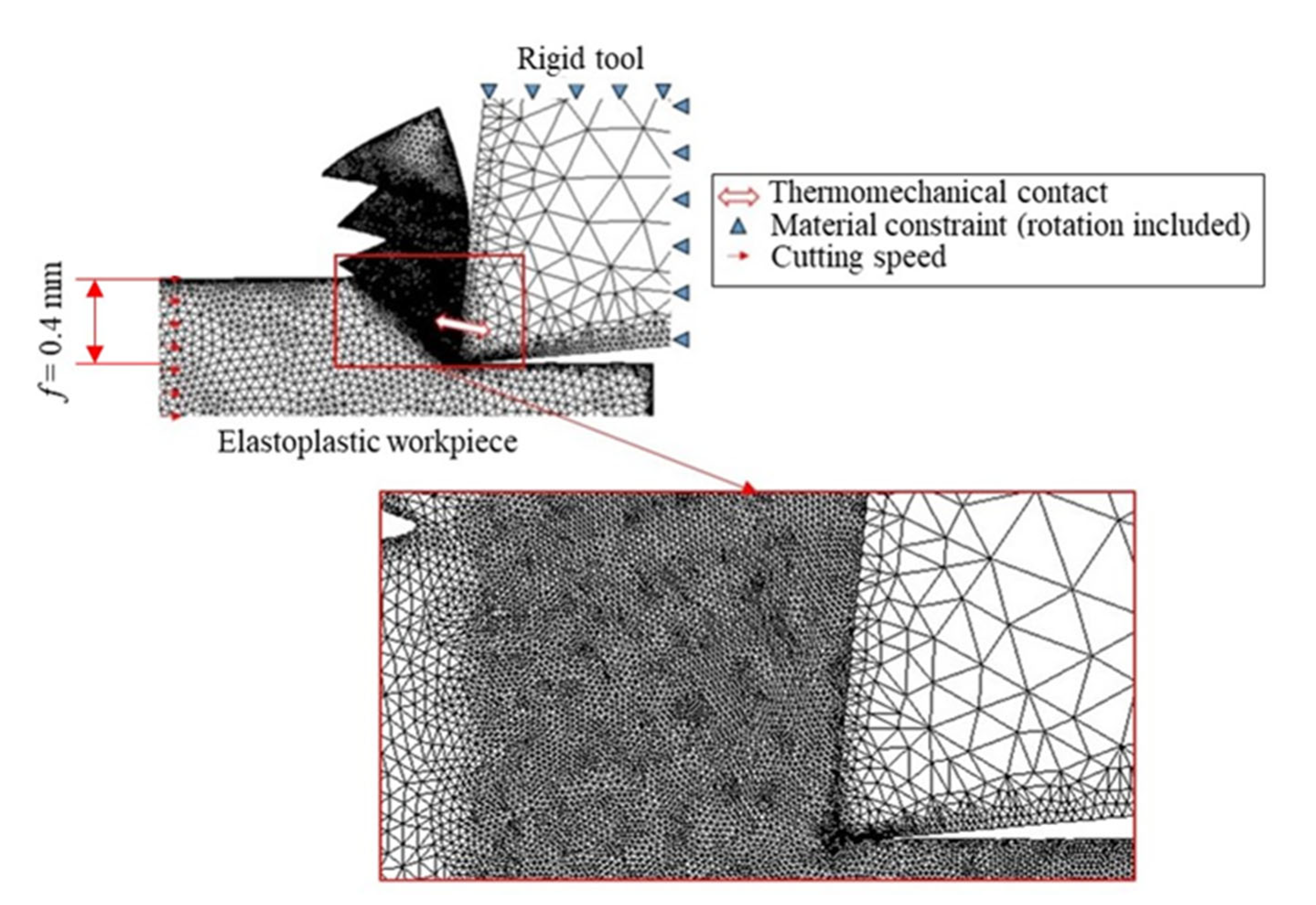
2. Finite Element Model

The FEM model employed is briefly explained in this section and more details can be found in [35]. The commercial software AdvantEdge-2D V7.502 (Third Wave Systems, Minneapolis, MN, USA) was chosen to carry out the simulations. AdvantEdge is a commercial finite element software which provides an easier approach than other generic software such as Abaqus to model the machining process. The software employs elastoplastic Lagrangian code with continuous remeshing and adaptive meshing. The remeshing technique ensures a minimum element size in the shear zone, where severe conditions (high strain, temperature and strain rate) are expected. The minimum element size was set to 2 µm to obtain accurate results, assuming that the material behaviour is homogenous. An example of the mesh with the boundary conditions is shown in Figure 1.

The tool is modelled as a rigid body, whereas the linear movement is imposed to the elastoplastic workpiece. The contact is modelled as a thermomechanical contact, allowing conduction heat transfer between the tool and the workpiece. The model assumes 2D deformation mode representative of the orthogonal cutting process.

To obtain reliable outputs, an appropriate selection of input parameters is a key aspect. Among all the flow stress laws presented in the literature, a comprehensive study was carried out by Ortiz de Zarate et al. [41]. They compared different machining outcomes using different flow stress laws coupled with a ductile failure law, concluding that the Johnson and Cook model (see Equation (1)) was accurate in reproducing the machining behavior. The model considers isotropic hardening, strain rate hardening and thermal softening as three independent phenomena without couplings, simplifying the simulations. The material constants are summarized in

Table 4. Johnson and Cook model parameters for Ti6Al4V alloy [10].

A (MPa)	B (MPa)	C	n	${\dot{\mathit{\epsilon }}}_{\mathbf{0}}$ (s−1)	Tmelt (°C)	m
1130	530	0.0165	0.39	1	1650	0.61

and they were taken from [35].

$$\sigma =\left[A+B{\left(\mathsf{\epsilon }\right)}^n\right]\left[1+C\ln \left(\frac{\dot{\epsilon }}{{\dot{\epsilon }}_0}\right)\right]\left[1-{\left(\frac{\left(T-T_0\right)}{\left(T_{melt}-T_0\right)}\right)}^m\right]$$

(1)

In addition, Ti6Al4V tends to generate segmented chips. A ductile failure law was thus introduced to model this segmentation as a two-stage physical-based equation in which Mohr-Coulomb’s law represents failure initiation, leading to a flow stress reduction. The damage is determined based on the accumulation of damage along a streamline, according to Equation (2). It was assumed that failure starts when D reaches a value of 1.

$$D={{\displaystyle \int }}_0^{{\epsilon }_f}\frac{d\epsilon }{{\epsilon }_f}$$

(2)

where ε is the equivalent plastic strain and ε_f the plastic strain to failure.

The plastic strain to failure can be expressed as a function of (ε_f,0)_T, the strain to failure under shear/torsion conditions; the stress triaxiality (η) and the stress triaxiality sensitivity constant (c). The relationship can be seen in Equation (3).

$${\epsilon }_f={\left({\epsilon }_{f,0}\right)}_T\exp \left(c\eta \right)$$

(3)

In addition, the strain to failure under shear/torsion is assumed to be dependent on the temperature as a linear function up to a critical temperature. Therefore, under the critical temperature (T_crit = 600 °C), the relationship can be expressed, as Equation (4) shows.

$${\left({\epsilon }_{f,0}\right)}_T={\epsilon }_{f,0}\left(1+aT\right)$$

(4)

where ${\epsilon }_{f,0}$ and a are material constants and T is the temperature.

If the accumulated damage value does not reach 1, the plastic behavior of the material is only modelled by the Johnson and Cook model (Equation (1)), whereas if this value is 1, the flow stress is given by Equation (5).

$${\sigma }_D=f\left(\eta ,T\right)\sigma$$

(5)

where the damaged flow stress, ${\sigma }_D$, depends on the reduction function caused by the damage and the flow stress given by Equation (1).

In addition, because of the healing effect, the damage will not affect the flow stress at temperatures higher than a critical one, defined as T_U. Below this critical temperature, the flow stress reduction is temperature dependent, as shown in Equation (6).

$$\begin{array}{cc}f\left(\eta ,T\right)=1,& T>T_{\mathrm{U}}\\ f\left(\eta ,T\right)=\tanh \left[-\sqrt{3}{\mu }_i\eta \right]+\left(1-\tanh \left[-\sqrt{3}{\mu }_i\eta \right]\right)\left(\frac{T-T_{\mathrm{L}}}{T_{\mathrm{U}}-T_{\mathrm{L}}}\right),& T_{\mathrm{L}}<T<T_{\mathrm{U}}\\ f\left(\eta ,T\right)=\tanh \left[-\sqrt{3}{\mu }_i\eta \right],& T<T_{\mathrm{L}}\end{array}$$

(6)

The material parameters employed in the ductile failure law are summarized in

Table 5. Damage and failure parameters for Ti6Al4V alloy [35].

${\mathit{\epsilon }}_{\mathit{f},0}$	a	c	${\mathit{\mu }}_{\mathit{i}}$	TL (°C)	TU (°C)
0.25	0.0012	−1.5	1	600	700

.

Both flow and ductile failure laws were implemented by user-defined subroutines programmed in Fortran language.

In addition, a sensitivity analysis was carried out analyzing the effect of ${\epsilon }_{f,0}$ on segmentation frequency so as to carry out the inverse analysis. Different values were analyzed, taking into consideration the possible values found in the literature for this parameter. A linear relationship was found between this parameter and the segmentation frequency. This linear relationship was also reproduced by the pitch. Based on this linear relationship, the simulations were launched again using the improved parameter.

The sticking-sliding model was selected to reproduce the friction and the friction coefficient was set to 1, according to the literature [42]. The thermal conductivity and heat capacity of the material were taken from literature [35], being, at room temperature, 6.7 W/mK and 2.3 MJ/m³, respectively. The heat capacity of the tool was notably reduced from the real physical value and set to 0.1 MJ/m³ in order to reduce the time needed to reach the steady state. Heat transfer coefficients were set as default, without coolant. The cutting conditions are shown in

Table 6. Experimental plan.

Tool	Ref.	TPUN 160308
	Rake angle, $\gamma$ (°)	6
	Clearance angle, $\alpha$ (°)	5
	Coating	Uncoated
	Edge radius, $r_e$ (µm)	25
Cutting conditions	Cutting speed, Vc (m/min)	2.5 and 7.5
	Feed, f (mm)	0.2 and 0.4
	Width, w (mm)	4
Lubrication	Type	Dry
Workpiece	Material	Ti6Al4V

. The workpiece height was set ten times higher than the feed for each condition to prevent possible effects of the boundary conditions on the results.

In order to validate the model, numerical results were also compared with those obtained from analytical equations reported in the literature. The difficulties of measuring workpiece temperature have led to different analytical equations to estimate it. One of the most successful and employed laws was proposed by Loewen and Shaw [51].

In short, the model assumes that the 90% of the plastic work is transformed into heat, proposing Equation (7).

$$T_{sz}=\frac{0.9}{1+1.328\sqrt{\frac{d_{\alpha }{\gamma }_{\mathrm{theo}}}{V_{c}f}}}\frac{\tau {\gamma }_{\mathrm{theo}}}{\rho c_p}+T_0$$

(7)

where T_sz is the average temperature in the shear zone, T₀ is the room temperature, $d_{\alpha }$ is the thermal diffusivity of the material, taken as 4 × 10⁻⁶ m²s⁻¹ according to [52], $\tau$ is the shear stress, ${\gamma }_{\mathrm{theo}}$ is the equivalent shear strain determined based on the model explained in [53], $\rho$ is the density of the material (4430 kg/m³) and c_p is the specific heat capacity (600 J/kgK according to [52]).

Boothroyd [54] proposed another easy model decomposing the shearing heat flux, depending on the thermal number (Peclet number), $Pe=f{V}_c/d_{\alpha }$. Thus, the temperature in the shear zone can be calculated according to Equation (8).

$$T_{sz}=\frac{1-\chi }{\rho c_p}\frac{\tau \cos \left(\gamma \right)}{\cos \left(\varphi -\gamma \right)\sin \varphi }+T_0$$

(8)

where $\chi$ is the proportion of the shearing flux that flows into the workpiece, defined by Equation (9), and $\varphi$ is the shear angle.

$$\begin{array}{c}\chi =0.5-0.35{\log }_{10}\left(Pe\tan \left(\varphi \right)\right);\mathrm{if}0.004\le Pe\tan \left(\varphi \right)\le 10\\ \chi =0.3-0.15{\log }_{10}\left(Pe\tan \left(\varphi \right)\right);\mathrm{otherwise}\end{array}$$

(9)

The shear angle for each cutting condition was experimentally estimated based on infrared images. Furthermore, the shear stress was taken from literature (613 MPa) and was in agreement with those obtained from the FEM [55].

3. Experimental Set-Up

Experimental tests were carried out in a vertical machine center Lagun CNC 8070 (Lagun Machinery S.L., Alava, Spain). The Ti6Al4V workpiece was clamped to the Kistler dynamometer 9129AA (Kistler Ibérica S.L, Barcelona, Spain). which was also clamped to the table, giving the linear movement to the workpiece. The tool holder was set in the spindle. The scheme of the set-up is shown in Figure 2. The experimental plan, cutting conditions and tool microgeometry are included in Table 6. Three repetitions were carried out under each condition. It should be noted that a fresh insert was employed for each test to avoid possible wear effects. Low values of cutting speeds were chosen as they are representative of the broaching process, a widely used process in Ti6Al4V manufacture. In addition, these low values facilitate the filming process, making it necessary to have lower sampling frequencies in order to capture chip segmentation. The feed was chosen high in order to have enough field of view to analyze the cutting process. The width of cut was set to 4 mm (10 times lower than the maximum feed) to reduce as much side flow as possible in order to be as close as possible to pure orthogonal cutting conditions. The machine stiffness (considering the whole system) is around 50 N/µm, although tool deflections were proven not to play a relevant role as the results obtained with the three repetitions were consistent. With regard to the cutting tool, a commercial one was chosen, given the cutting geometry listed in Table 6. The edge radius was measured with the Alicona IFG4 profilometer (Bruker Alicona, Graz, Austria) with 10× magnification.

The sampling frequency of the dynamometer was 5000 Hz. Thermal fields were recorded through a Flir Titanium 550 m infrared camera (Teledyne FLIR, Wilsonville, OR, USA) located at 30 mm of the shear zone, equipped with a macroscopic lens giving a spatial resolution of 1 px² = 10 μm². The sampling frequency of the thermal imaging was 1000 Hz. The process was also filmed with a high-speed camera Photron Fastcam APX-RS 250 K (Photron Europe Limited, Wycombe, UK) and a sampling frequency of 9000 Hz to understand more in depth the mechanisms of chip formation.

The surface to be filmed was previously painted black in order to ensure the highest possible emissivity. The temperature variation on the shear zone was obtained through different measurement points (3 px × 3 px) located at different positions of the shear zone. An emissivity value of 0.8 was set to determine the temperature values. Nevertheless, it was observed that variations lower than ±20 °C were expected by varying the emissivity between 0.6 and 1, in agreement with [28]. The apparent reflected temperature was set to 25 °C and its effect was observed to be negligible under the conditions analyzed as the temperatures reached were notably higher.

The chip morphology was measured by mounting it on resin, followed by a mechanical polishing for optical microscopy analysis.

The material employed was the widely used aeronautical alloy Ti6Al4V, provided as a solid hot rolled bar with a diameter of 80 mm in the annealed condition. The initial microstructure of the sample was revealed with Kroll’s reagent and shows a microstructure with primary $\alpha$ grains and $\alpha +\beta$ colonies (see Figure 3). The material as received had a grain size of 10.5 ASTM, and the measured microhardness was 350 HV for an applied load of 50 g. The density of the material was 4430 kg/m³ and the chemical composition is given in

Table 7. Chemical composition of the Ti6Al4V alloy.

Element	V	Al	Fe	C	O	N	Ti
Weight (%)	4.05	6.36	0.16	0.015	0.019	0.006	Bal.

.

4. Results

In this section, experimental values of workpiece temperature, cutting forces and chip morphology obtained under the conditions summarized in Table 6 are explained. The temperature in the shear zone was obtained at different positions and different cutting times in order to obtain a representative average of the temperature in the shear zone, as shown in Figure 4.

During orthogonal cutting of Ti6Al4V, the crack is generated close to the tool, and it suddenly propagates to the rest of the shear zone, causing a drastic failure. In terms of temperature, this phenomenon could be observed as a concentration of heat, which is due to a coupling between severe strain and crack, close to the tool. This heat then suddenly spreads to the rest of the shear zone, as Figure 5 shows. Taking into consideration that the sampling frequency of the thermal camera (1000 Hz) was not able to capture the sudden increase in the temperature of the shear zone, it is clear that this behavior was due to a crack propagation (mechanical phenomenon) rather than a heat propagation by conduction along the shear zone. This was also corroborated thanks to the high-speed filming (also included in Figure 5); it can be seen that, at the beginning of the cutting process, the crack starts close to the edge radius and then suddenly spreads to the rest of the shear zone.

Because of this phenomenon, temperature notably varies along the shear zone; however, temperature frequency along the shear zone was observed to be independent on the selected point, as Figure 6 shows.

The temperature in the shear zone was observed to increase with the cutting speed (Figure 7), whereas higher amplitudes of oscillation ($∆T_{\mathrm{SZ}}$) were measured at high feeds when cutting speed was 7.5 m/min.

Cutting force was also measured, as shown in Figure 8. As expected, the cutting force increased with the feed. In addition, no remarkable effect of the cutting speed was found with regard to cutting forces. This is assumed to be due to the fact that under these cutting conditions, at low cutting speeds, thermal and strain rate effects are assumed to be low, not having remarkable influence on cutting forces [19]. Regarding the amplitude of oscillation, $∆F_c$ was higher at the highest feed.

It was measured that when the cutting force reached a minimum value, the workpiece temperature in the shear zone was at a maximum. This phenomenon could be observed in Figure 9. The increase on the cutting force yields to higher strains within the shear zone, then, when this plastic strain reaches a critical value (damage equal to 1) the crack starts, causing a notable reduction on the cutting force. The plastic work is converted into heat, implying a localized and fast temperature rise in the shear zone. This implies that cutting force and temperature signals should be in counterphase, which was experimentally observed.

Temperature and cutting force frequency could be a useful input to be compared with numerical simulations to validate the accuracy of the numerical model, as this was observed to occur under different cutting conditions. In addition, it is worth mentioning that temperature values could be notably lower than those reported by the numerical model as the load modes were different: plane stress in the visible surface and plane strain in the simulation. The measurements of the temperature were carried out on the visible surface, which could suffer from lateral expansion (side flow), resulting in a plane stress mode. In addition, thermal losses could cause the measured face to cool. These two reasons could explain the slightly different values obtained when comparing the experimental ones with those obtained from the numerical model, assumed to be subjected to plane strain conditions representative of the orthogonal cutting process.

Finally, chip morphology in terms of pitch value (distance peak to peak in a chip) and chip thickness (average and oscillation amplitude, $∆h_c$) were experimentally determined (see Figure 10).

It can be seen in Figure 11 that the pitch value increases with the feed, whereas it was not very sensitive to cutting speed changes. In addition, it is worth noting that the higher the oscillation amplitude of the cutting forces, the higher the pitch values that were observed, which means higher segmentation. This issue can also be observed by oscillations in chip thickness. In this sense, higher pitch values are related to lower segmentation frequencies. Concerning chip thickness, a notable increase was found with the feed, as expected. In addition, no remarkable variation when the cutting speed is modified was found, which is in agreement with the cutting force measurement shown in Figure 11 It was also observed that temperature oscillation frequency increases with cutting speed and decreases with feed.

5. Discussion

In this section, the experimental results previously shown are compared with the numerical results obtained with AdvantEdge-2D.

5.1. Model Validation

In order to compare these results with numerical simulations, first, it was demonstrated that the model was able to reproduce the thermal aspects concerning orthogonal cutting. This is shown in Figure 12. In addition, the experimental observation that temperature starts increasing close to the tool was also reproduced.

The temperature values obtained were plotted against the cutting severity. This is, the product Vc f, in m²min⁻¹, and this parameter is widely used to analyze the influence of the cutting speed and the feed on different outcomes. The obtained results are shown in Figure 13.

As can be observed, predicted values, regardless of numerical or analytical, were higher than the ones measured with the infrared camera. First, it is worth mentioning that the measurements were made based on the visible surface, that is, under plane stress measurements, whereas both numerical and analytical approaches were based on a plane strain assumption. Therefore, thermal losses could play a relevant role and the temperature inside the workpiece (plane strain) could be notably higher than the one measured. This was stated, for instance, by [24], observing a gap higher than 100 °C between the visible face and the center of the tool.

5.2. Ductile Failure Model Validation

After proving the capability of the model of reproducing thermal aspects of the cutting process, it was proved to be able to reproduce chip segmentation. Taking into consideration the chip morphology, an example of the accuracy of the predictions is shown in Figure 14. As can be seen, the chip segmentation is well reproduced by the numerical model thanks to the implementation of the ductile failure model. However, the pitch (which is associated with the segmentation frequency) is underpredicted.

As was shown above, when the cutting force reached a minimum value, the workpiece temperature along the shear zone was at a maximum. This phenomenon was reproduced by the numerical model, as shown in Figure 15 (the temperature shown in the plot was taken from a point located close to the tool).

Therefore, it was proved that the proposed ductile failure model describes the different physical phenomena occurring during the cutting process properly, as FEM predictions were reproduced by experimental measurements. The other experimental outcomes were also compared with those from the FEM, as Figure 16 shows.

It can be seen that the simulated segmentation frequencies were notably higher than those measured, being, in some cases (V_c = 7.5 m/min and f = 0.2 mm), more than 100% higher. This aspect is in agreement with the lower pitch values reported by the numerical model. These discrepancies were more noticeable at 7.5 m/min. Nevertheless, it is worth mentioning that the trends were well predicted by the numerical model. Cutting forces were also well predicted, with average prediction errors lower than 20%, taking into consideration the whole set of cutting conditions. Finally, prediction error, concerning chip geometry (chip thickness and $∆h_c$), was lower than 6%, whereas the pitch values were underpredicted for the whole set of cutting conditions, with a prediction error up to 100% in low feed cases.

6. Inverse Approach

According to [41], the effect of the flow stress law on the pitch (and, thus, on the segmentation frequency) was observed to be negligible, as chip segmentation is assumed to be governed by the lack of ductility of the material under these conditions. However, notable influence was found regarding the ductile failure law, especially when ε_f,0 (failure initiation parameter) is modified [42], thereby making this outcome a useful input to optimize the material model implemented.

Therefore, an inverse approach was taken to improve the accuracy of predictions based on segmentation frequency. First, different simulations were launched, varying the value of ε_f,0 between 0.25 (the reference value given in [35]) and 0.5 (the highest value found in literature for this parameter [56,57,58]) under the condition of V_c = 7.5 m/min and f = 0.2 mm as it corresponds to the worst condition predicted. According to [42], the increase in this parameter leads to higher pitches and, thus, lower frequencies. This behavior is shown in Figure 17.

The effect of this parameter over cutting forces, cutting temperature and chip thickness was analyzed, observing how this parameter has no remarkable effect on force and cutting temperature predictions, considering neither the average value nor the amplitudes of the oscillations (see Figure 18).

In addition, by increasing this parameter, a slight increase in the average chip thickness was obtained, not affecting the magnitude of the chip thickness amplitude. However, this variation does not have any influence on the accuracy of the predictions. It is worth mentioning that chip shape and curvature was slightly modified by increasing ε_f,0.

A linear relationship under the tested cutting conditions was found between the parameter ε_f,0, the segmentation frequency and the pitch value, as Figure 19 shows. It is worth mentioning that with ε_f,0 = 0.5, no segmentation was observed. Based on this linear regression, the ε_f,0 for a segmentation frequency of 300 Hz (experimental value obtained) was 0.41. Therefore, based on this procedure, the analyzed cutting conditions were launched again, taking into consideration this value.

After performing the optimization, it can be seen that the errors in frequency and pitch predictions were notably reduced, not only in the condition employed to optimize the law, but also in the rest of the cutting conditions analyzed (see Figure 20).

For instance, for V_c = 7.5 m/min and f =0.2 mm, the relative error $\left(\frac{\left|Exp-Pred\right|}{Exp}\right)$ in frequency and pitch prediction is reduced from 100% to less than 10%, whereas for V_c = 2.5 m/min and f = 0.4 mm, the prediction error is reduced from 30% to 7%. The average prediction error was 9%.

7. Conclusions

The ductile failure law of the material has been improved by using inverse simulation and based on infrared measurements in order to improve the accuracy on chip segmentation prediction when cutting Ti6Al4V. Hence, the following conclusions can be drawn:

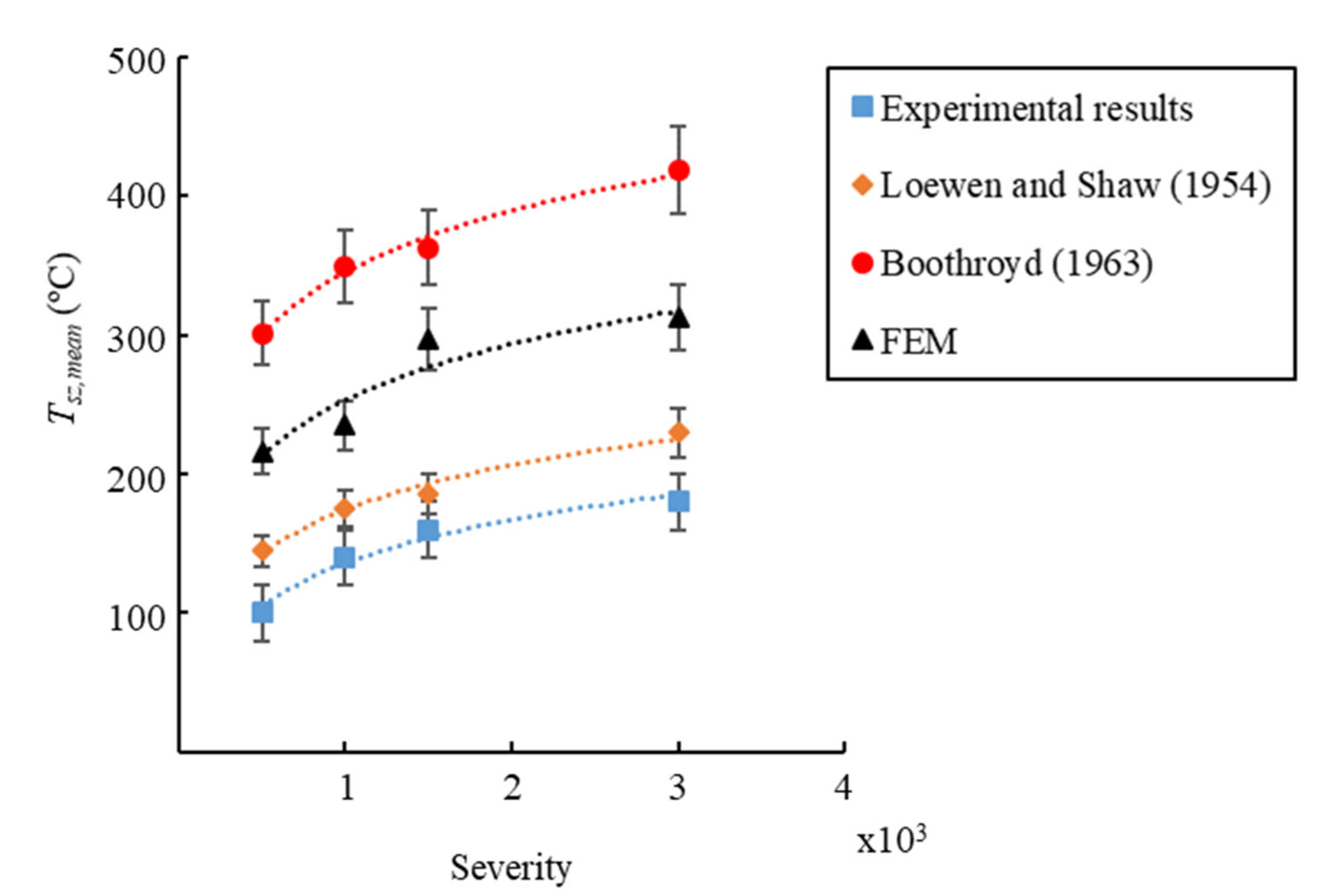
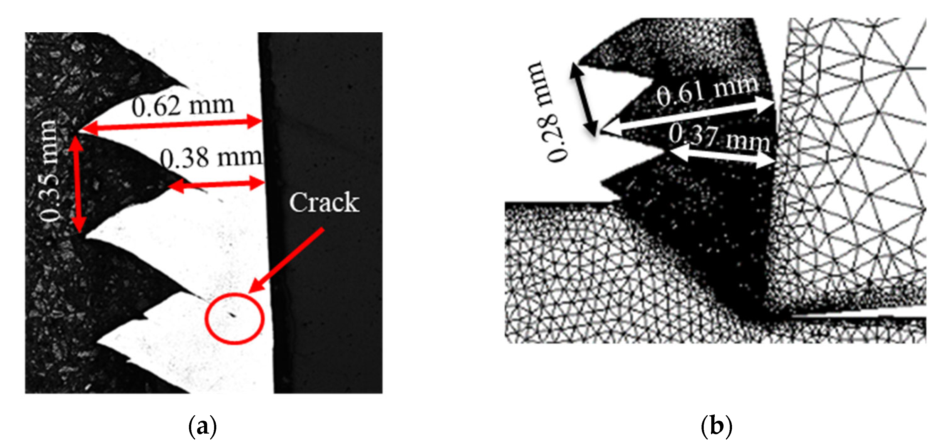
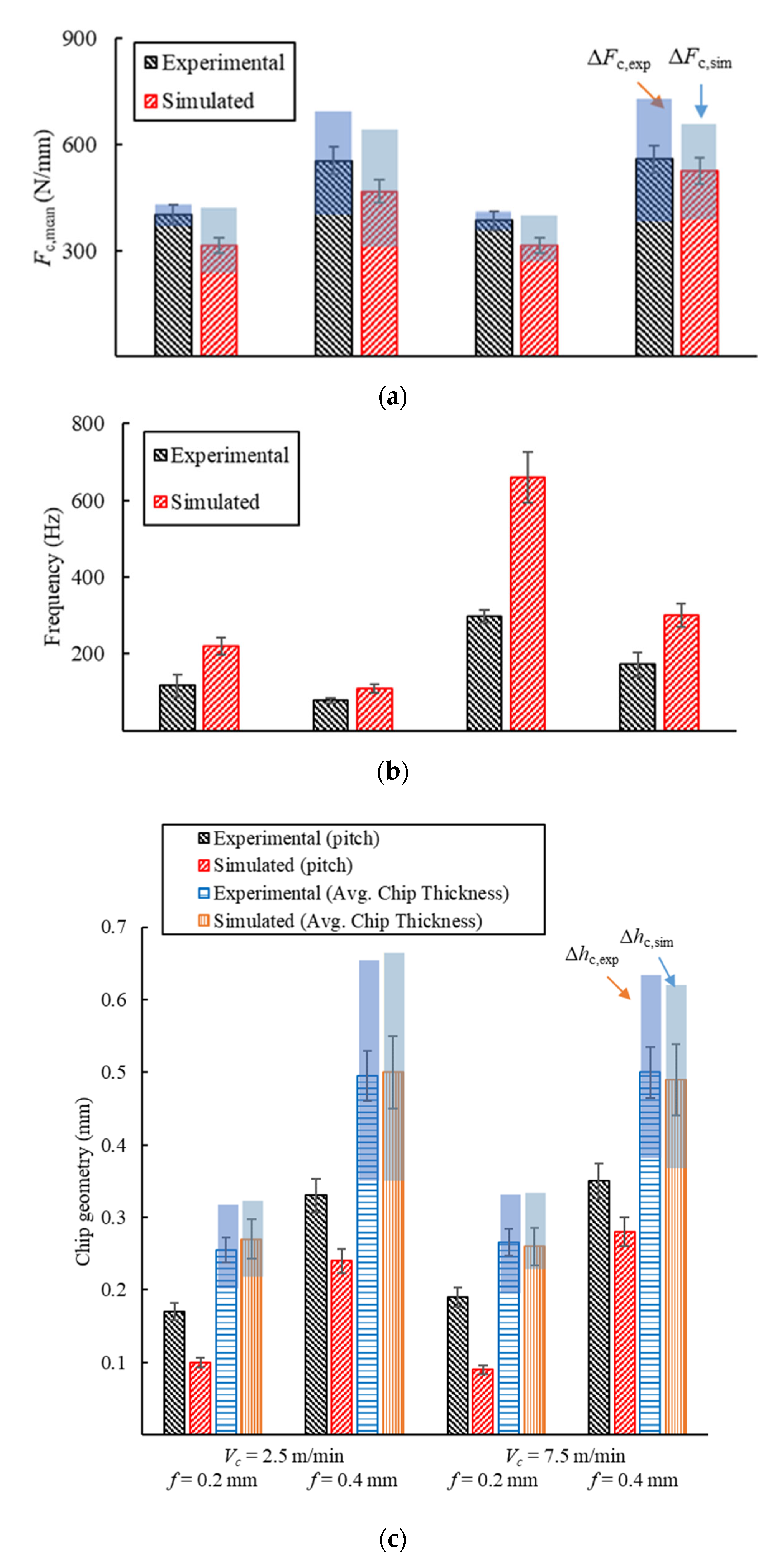
• The numerical model employed is able to reproduce chip segmentation and to simulate forces and the shape of thermal fields accurately. Therefore, the ductile failure model implemented reproduced the physical phenomena occurring during cutting.
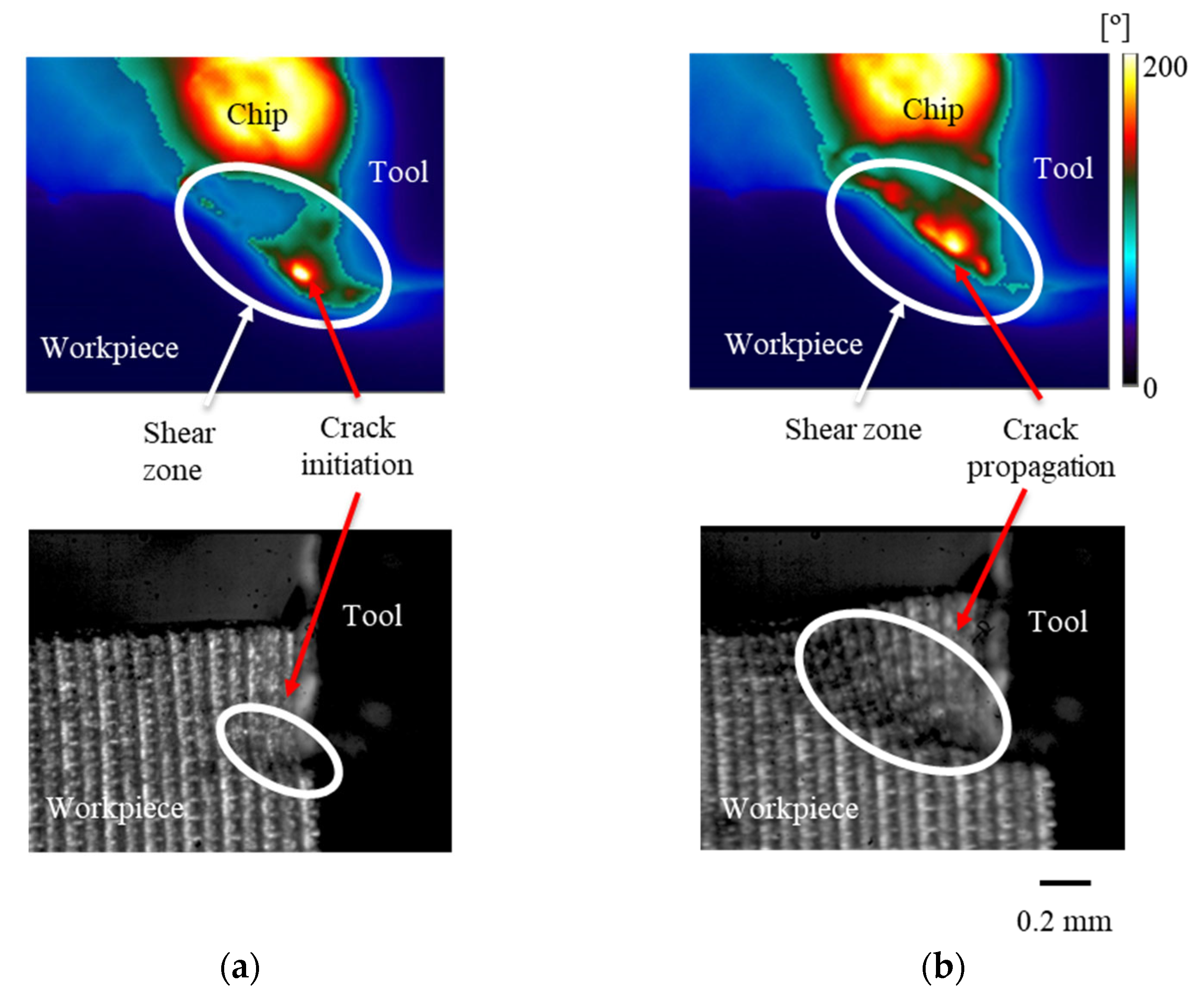
• It was observed that at low cutting speeds, the crack starts close to the tool and then suddenly spreads to the rest of the shear zone, causing drastic failure and proving the lack of ductility of the material. This plastic work is transformed into heat, causing a sudden temperature rise observable by the thermal camera.
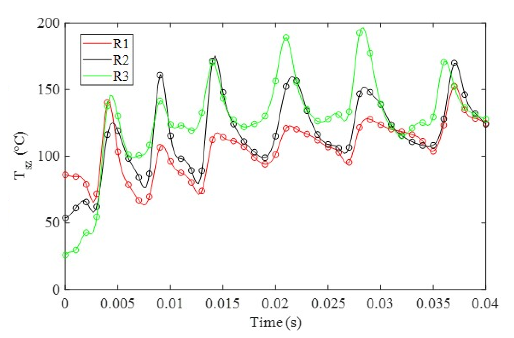
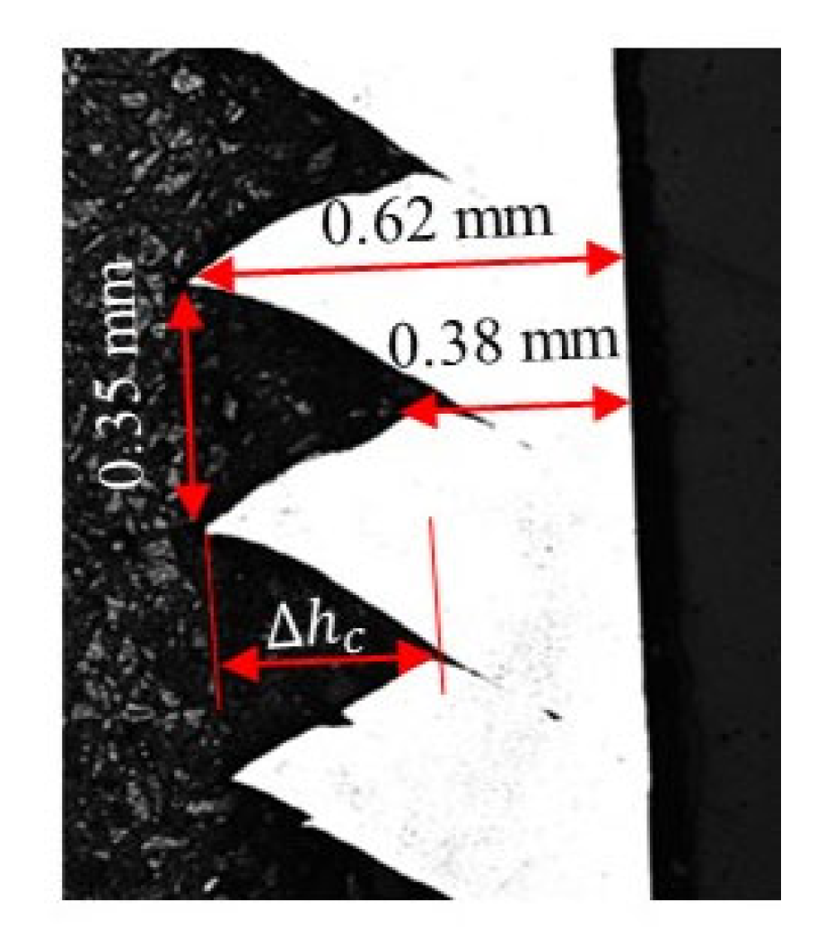
• Chip segmentation produced during machining of Ti6Al4V leads to the oscillation of relevant outcomes such as cutting forces, chip thickness and workpiece temperature.
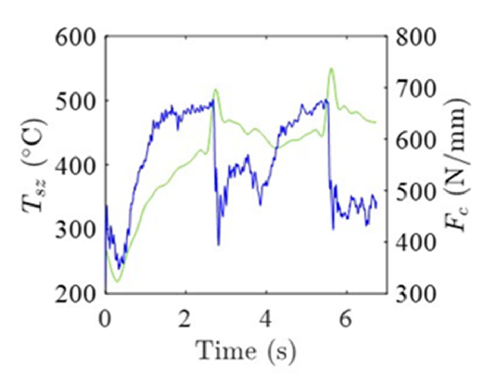
• The oscillation frequency was observed to be equal based on cutting force and workpiece temperature measurements while signals were in counterphase. This frequency is identified as an interesting input to be considered so as to optimize the numerical model.
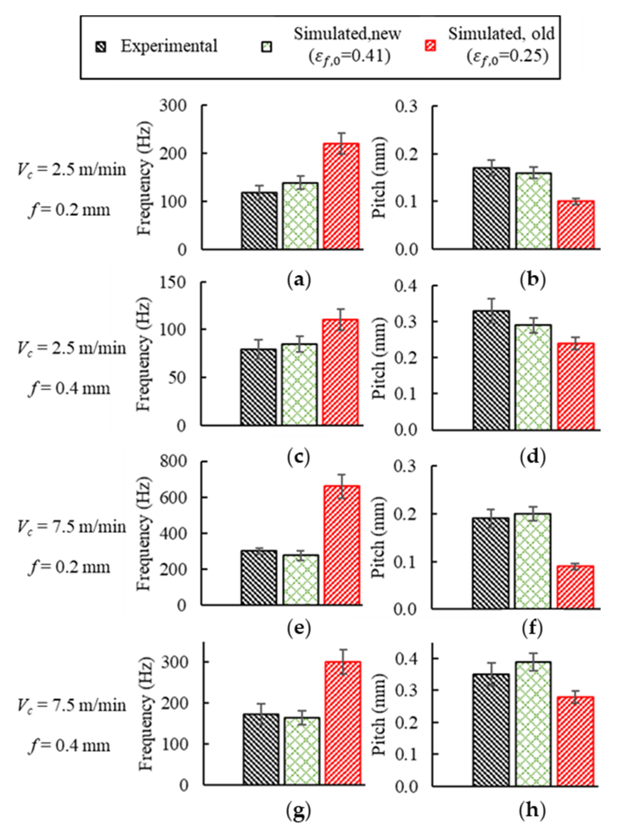
• The ductile failure law was optimized by using inverse methodology by optimizing the parameter ε_f,0, reducing the error in the frequency prediction from more than 100% to less than 10% in the worst case, maintaining the accuracy in the rest of the predictions.

References

1. Ezugwu, E. Key improvements machining Difficult-cut aerospace superalloys. Int. J. Mach. Tools Manuf. 2005, 45, 1353–1367. [Google Scholar] [CrossRef]
2. Ivester, R.W.; Kennedy, M.; Davies, M.; Stevenson, R.; Thiele, J.; Furness, R.; Athavale, S. Assessment machining models: Progress report. Mach. Sci. Technol. 2000, 4, 511–538. [Google Scholar] [CrossRef]
3. Arrazola, P.J.; Özel, T.; Umbrello, D.; Davies, M.; Jawahir, I. Recent advances modelling Metal machining Processes. CIRP Ann. 2013, 62, 695–718. [Google Scholar] [CrossRef]
4. Melkote, S.N.; Grzesik, W.; Outeiro, J.; Rech, J.; Schulze, V.; Attia, H.; Arrazola, P.-J.; M’Saoubi, R.; Saldana, C. Advances material Friction data modelling Metal machining. CIRP Ann. 2017, 66, 731–754. [Google Scholar] [CrossRef] [Green Version]
5. Harzallah, M.; Pottier, T.; Senatore, J.; Mousseigne, M.; Germain, G.; Landon, Y. Numerical experimental investigations Ti6Al4V chip Generation thermo-mechanical couplings Orthogonal cutting. Int. J. Mech. Sci. 2017, 134, 189–202. [Google Scholar] [CrossRef] [Green Version]
6. Hor, A.; Morel, F.; Lebrun, J.-L.; Germain, G. Modelling, identification application Phenomenological constitutive Laws large strain rate Temperature range. Mech. Mater. 2013, 64, 91–110. [Google Scholar] [CrossRef] [Green Version]
7. Militzer, M.; Botton, G.; Chen, L.-Q.; Howe, J.; Sinclair, C.; Zurob, H. Phase transformations kinetics of ti-6al-4v during very fast heating using in-situ high-energy x-ray diffraction (HE-XRD). In Proceedings of the International Conference on Solid-Solid Phase Transformations in Inorganic Materials, Whistler, BC, Canada, 28 June–3 July 2015. [Google Scholar]
8. Shrot, A.; Bäker, M. Is it Possible identify Johnson-Cook law parameters Machining simulations? Int. J. Mater. Form. 2010, 3, 443–446. [Google Scholar] [CrossRef]
9. Pujana, J.; Arrazola, P.; M’saoubi, R.; Chandrasekaran, H. Analysis inverse identification Constitutive equations Applied orthogonal cutting process. Int. J. Mach. Tools Manuf. 2007, 47, 2153–2161. [Google Scholar] [CrossRef]
10. Shrot, A.; Bäker, M. Determination Johnson–Cook parameters Machining simulations. Comput. Mater. Sci. 2012, 52, 298–304. [Google Scholar] [CrossRef]
11. Daoud, M.; Jomaa, W.; Chatelain, J.F.; Bouzid, A. A machining Based methodology identify material constitutive lawFiniteelementSimulation. Int. J. Adv. Manuf. Technol. 2015, 77, 2019–2033. [Google Scholar] [CrossRef]
12. Agmell, M.; Ahadi, A.; Ståhl, J.-E. Identification plasticity constants Orthogonal cutting inverse analysis. Mech. Mater. 2014, 77, 43–51. [Google Scholar] [CrossRef]
13. Klocke, F.; Lung, D.; Buchkremer, S. Inverse identification constitutive equation Inconel718 AISI 1045 FE machining Simulations. Procedia Cirp 2013, 8, 212–217. [Google Scholar] [CrossRef] [Green Version]
14. Sartkulvanich, P.; Koppka, F.; Altan, T. Determination flow stress Metalcutting Simulation progress report. J. Mater. Process. Technol. 2004, 146, 61–71. [Google Scholar] [CrossRef]
15. Razanica, S.; Malakizadi, A.; Larsson, R.; Cedergren, S.; Josefson, B. FE modeling simulation Machining Alloy718 based ductile continuum damage. Int. J. Mech. Sci. 2020, 171, 105375. [Google Scholar]
16. Malakizadi, A.; Cedergren, S.; Sadik, I.; Nyborg, L. Inverse identification flow stress Metal cutting Process using Response Surface Methodology. Simul. Model. Pract. Theory 2016, 60, 40–53. [Google Scholar] [CrossRef]
17. Hardt, M.; Schraknepper, D.; Bergs, T. Investigations Application Downhill Simplex Algorithm Inverse Determination Material Model Parameters FE-Machining Simulations. Simul. Model. Pract. Theory 2021, 107, 102214. [Google Scholar] [CrossRef]
18. Franchi, R.; Del Prete, A.; Umbrello, D. Inverse analysis Procedure determine flow stress Friction data finite element modeling Machining. Int. J. Mater. Form. 2017, 10, 685–695. [Google Scholar] [CrossRef]
19. Zhang, D.; Zhang, X.; Ding, H. Inverse identification material plastic constitutive parameters based DIC determined Workpiece deformation Fields orthogonal cutting. Procedia CIRP 2018, 71, 134–139. [Google Scholar] [CrossRef]
20. Zhang, X.-M.; Zhang, K.; Zhang, D.; Outeiro, J.; Ding, H. New In Situ Imaging Based Methodology Identify Material Constitutive Model Coefficients Metal Cutting Process. J. Manuf. Sci. Eng. 2019, 141. [Google Scholar] [CrossRef] [Green Version]
21. Thimm, B.; Steden, J.; Reuber, M.; Christ, H.-J. Using Digital Image Correlation Measurements Inverse Identification Constitutive Material Parameters applied Metal Cutting Simulations. Procedia CIRP 2019, 82, 95–100. [Google Scholar] [CrossRef]
22. Davies, M.; Ueda, T.; M’saoubi, R.; Mullany, B.; Cooke, A. On measurement Temperature material removal processes. CIRP Ann. 2007, 56, 581–604. [Google Scholar] [CrossRef]
23. Sutter, G.; Faure, L.; Molinari, A.; Ranc, N.; Pina, V. An experimental Technique measurement Temperature fields orthogonal cutting High speed Machining. Int. J. Mach. Tools Manuf. 2003, 43, 671–678. [Google Scholar] [CrossRef] [Green Version]
24. Soler, D.; Aristimuño, P.; Saez-de-Buruaga, M.; Garay, A.; Arrazola, P. New calibration Method measure rake face temperature Tool dry orthogonal cutting using thermography. Appl. Therm. Eng. 2018, 137, 74–82. [Google Scholar] [CrossRef]
25. Dinc, C.; Lazoglu, I.; Serpenguzel, A. Analysis thermal fields Orthogonal machining infrared imaging. J. Mater. Process. Technol. 2008, 198, 147–154. [Google Scholar] [CrossRef]
26. Heigel, J.C.; Whitenton, E.; Lane, B.; Donmez, M.A.; Madhavan, V.; Moscoso-Kingsley, W. Infrared measurement temperature Tool–chip interface While machining Ti–6Al–4V. J. Mater. Process. Technol. 2017, 243, 123–130. [Google Scholar] [CrossRef] [Green Version]
27. Sutter, G.; Ranc, N. Temperature fields chip High speed Orthogonal cutting—An Experimental investigation. Int. J. Mach. Tools Manuf. 2007, 47, 1507–1517. [Google Scholar] [CrossRef] [Green Version]
28. Zhang, F.; Yu, K.; Zhang, K.; Liu, Y.; Xu, K.; Liu, Y. An emissivity Measurement apparatus infrared spectrum. Infrared Phys. Technol. 2015, 73, 275–280. [Google Scholar] [CrossRef]
29. Harzallah, M.; Pottier, T.; Gilblas, R.; Landon, Y.; Mousseigne, M.; Senatore, J. Thermomechanical coupling Investigation Ti-6Al-4V orthogonal cutting: Experimental Numerical confrontation. Int. J. Mech. Sci. 2020, 169, 105322. [Google Scholar] [CrossRef]
30. Cotterell, M.; Ares, E.; Yanes, J.; López, F.; Hernandez, P.; Peláez, G. Temperature Strain Measurement Chip Formation Orthogonal Cutting Conditions Applied Ti6Al4V. Procedia Eng. 2013, 63, 922–930. [Google Scholar] [CrossRef] [Green Version]
31. Jawahir, I.; Brinksmeier, E.; M’saoubi, R.; Aspinwall, D.; Outeiro, J.; Meyer, D.; Umbrello, D.; Jayal, A. Surface integrity material removal processes: Recent advances. CIRP Ann. 2011, 60, 603–626. [Google Scholar] [CrossRef]
32. Komanduri, R.; Hou, Z. A review experimental techniques Measurement heat Temperatures generated some manufacturing processes Tribology. Tribol. Int. 2001, 34, 653–682. [Google Scholar] [CrossRef]
33. M’Saoubi, R.; Axinte, D.; Soo, S.L.; Nobel, C.; Attia, H.; Kappmeyer, G.; Engin, S.; Sim, W.-M. High performance Cutting advanced aerospace alloys Composite materials. CIRP Ann. 2015, 64, 557–580. [Google Scholar] [CrossRef]
34. Ulutan, D.; Ozel, T. Machining induced Surface integrity titanium Nickel alloys A review. Int. J. Mach. Tools Manuf. 2011, 51, 250–280. [Google Scholar] [CrossRef]
35. Childs, T.H.; Arrazola, P.-J.; Aristimuno, P.; Garay, A.; Sacristan, I. Ti6Al4V metal Cutting chip Formation experiments modelling Wide range cutting speeds. J. Mater. Process. Technol. 2018, 255, 898–913. [Google Scholar] [CrossRef] [Green Version]
36. Ye, G.; Jiang, M.; Xue, S.; Ma, W.; Dai, L. On instability Chip flow high-speed machining. Mech. Mater. 2018, 116, 104–119. [Google Scholar] [CrossRef]
37. Ducobu, F.; Rivière-Lorphèvre, E.; Filippi, E. Material constitutive Model chip separation criterion influence Modeling Ti6Al4V machining Experimental validation strictly orthogonal cutting condition. Int. J. Mech. Sci. 2016, 107, 136–149. [Google Scholar] [CrossRef]
38. Kishawy, H.A.; Hosseini, A. Machining Difficult-Cut Materials; Springer: Berlin, Germany, 2019. [Google Scholar]
39. Elbestawi, M.; Srivastava, A.; El-Wardany, T. A model chip formation Machining hardened steel. CIRP Ann. 1996, 45, 71–76. [Google Scholar] [CrossRef]
40. Ortiz-de-Zarate, G.; Sela, A.; Soriano, D.; Soler, D.; Aristimuño, P.; Arrazola, P. Influence chip segmentation Ti64 topography Machined surface. In Proceedings of the AIP Conference Proceedings; AIP Publishing LLC: Melville, NY, USA, 2019; Volume 2113, p. 080022. [Google Scholar]
41. Ortiz-de-Zarate, G.; Sela, A.; Ducobu, F.; Saez-de-Buruaga, M.; Soler, D.; Childs, T.; Arrazola, P. Evaluation different flow stress laws coupled Physical based Ductile failure Criterion modelling Chip formation Process Ti-6Al-4VBroachingconditions. Procedia CIRP 2019, 82, 65–70. [Google Scholar] [CrossRef]
42. Ortiz-de-Zarate, G.; Sela, A.; Madariaga, A.; Childs, T.; Arrazola, P. Sensitivity analysis input parameters Physical based Ductile failure Model Ti-6Al-4V Prediction surface integrity. Procedia CIRP 2020, 87, 533–538. [Google Scholar] [CrossRef]
43. Johnson, G.R.; Cook, W.H. Fracture characteristics three metals subjected Various strains, Strain rates, Temperatures pressures. Eng. Fract. Mech. 1985, 21, 31–48. [Google Scholar] [CrossRef]
44. Wilkins, M.; Streit, R.; Reaugh, J. Cumulative Strain Damage Model Ductile Fracture: Simulation Prediction Engineering Fracture Tests; Science Applications, Inc.: San Diego, CA, USA, 1980. [Google Scholar]
45. Wierzbicki, T.; Xue, L. On Effect Third Invariant Stress Deviator Ductile Fracture; Impact and Crashworthiness Laboratory: Cambridge, MA, USA, 2005; Volume 136. [Google Scholar]
46. Lian, J.; Sharaf, M.; Archie, F.; Münstermann, S. A hybrid Approach modelling Plasticity failure behaviour Advanced high Strength steel Sheets. Int. J. Damage Mech. 2013, 22, 188–218. [Google Scholar] [CrossRef]
47. Bao, Y.; Wierzbicki, T. On fracture Locus equivalent strain Stress triaxiality Space. Int. J. Mech. Sci. 2004, 46, 81–98. [Google Scholar] [CrossRef]
48. Bao, Y.; Wierzbicki, T. On cut Value negative triaxiality Fracture. Eng. Fract. Mech. 2005, 72, 1049–1069. [Google Scholar] [CrossRef]
49. Cheng, W.; Outeiro, J.; Costes, J.-P.; M’Saoubi, R.; Karaouni, H.; Astakhov, V. A constitutive Model Ti6Al4V considering State stress Strain rate Effects. Mech. Mater. 2019, 137, 103103. [Google Scholar] [CrossRef] [Green Version]
50. Liu, J.; Bai, Y.; Xu, C. Evaluation ductile fracture models Finite element Simulation metal cutting processes. J. Manuf. Sci. Eng. 2014, 136. [Google Scholar] [CrossRef]
51. Loewen, E.G.; Shaw, M.C. On analysis Cutting tool Temperatures. Tras. ASME 1954, 76, 217. [Google Scholar]
52. Miloševi, N.; Aleksi, I. Thermophysical properties solid phase Ti-6Al-4V alloy Wide temperature Range. Int. J. Mater. Res. 2012, 103, 707–714. [Google Scholar] [CrossRef]
53. Bai, W.; Sun, R.; Roy, A.; Silberschmidt, V.V. Improved analytical Prediction chip formation Orthogonal cutting titanium alloy Ti6Al4V. Int. J. Mech. Sci. 2017, 133, 357–367. [Google Scholar] [CrossRef] [Green Version]
54. Boothroyd, G. Temperatures orthogonal metal cutting. Proc. Inst. Mech. Eng. 1963, 177, 789–810. [Google Scholar]
55. Budak, E.; Altintas, Y.; Armarego, E. Prediction milling force coefficients Orthogonal cutting Data. J. Manuf. Sci. Eng. 1996, 118, 216–224. [Google Scholar] [CrossRef]
56. Allahverdizadeh, N.; Gilioli, A.; Manes, A.; Giglio, M. An experimental numerical study Damage characterization Ti–6AL–4V titanium alloy. Int. J. Mech. Sci. 2015, 93, 32–47. [Google Scholar] [CrossRef]
57. Hammer, J.T. Plastic Deformation Ductile Fracture Ti6Al4V Various Loading Conditions. Master’s Thesis, The Ohio State University, Columbus, OH, USA, 2012. [Google Scholar]
58. Simha, C.H.M.; Williams, B.W. Modelingfailure Ti-6Al-4V using damage mechanics incorporating effects Anisotropy, rate temperature Strength. Int. J. Fract. 2016, 198, 101–115. [Google Scholar] [CrossRef]
Figure 1. Example of the mesh for the orthogonal cutting case with special focus on the shear zone. f represents the feed or uncut chip thickness in orthogonal cutting.
Metals 11 01154 g001
Figure 2. Experimental set up to carry out the orthogonal tests.
Metals 11 01154 g002
Figure 3. Initial microstructure of the Ti6Al4V employed.
Metals 11 01154 g003
Figure 4. Example of a thermogram. R1, R2 and R3 represent 3 px × 3 px measurement points located along the shear zone. Cutting speed Vc = 7.5 m/min and feed f = 0.4 mm.
Metals 11 01154 g004
Figure 5. Thermal fields and high-speed images during orthogonal cutting of Ti6Al4V. (a) Crack initiation. (b) Crack propagation. Vc = 7.5 m/min and f = 0.4 mm.
Metals 11 01154 g005
Figure 6. Temperature evolution on the visible surface during orthogonal cutting of Ti6Al4V at different points of the shear zone (see Figure 4). Vc = 7.5 m/min and f = 0.4 mm.
Metals 11 01154 g006
Figure 7. Effect of cutting conditions on workpiece temperature in the shear zone (amplitude of oscillation, T S Z , also included).
Metals 11 01154 g007
Figure 8. Effect of cutting conditions on cutting force (amplitude of oscillation, F c , also included).
Metals 11 01154 g008
Figure 9. Experimental measurements of temperature and force evolution during orthogonal cutting of Ti6Al4V. (a) Vc = 2.5 m/min and f = 0.4 mm; (b) Vc = 7.5 m/min and f = 0.4 mm.
Metals 11 01154 g009
Figure 10. Chip geometry measurement: Maximum chip thickness, minimum chip thickness and pitch. Vc = 7.5 m/min and f = 0.4 mm.
Metals 11 01154 g010
Figure 11. Effect of cutting conditions on oscillation frequency and chip geometry (experimental results).
Metals 11 01154 g011
Figure 12. Experimental (a) and simulated (b) thermal fields during orthogonal cutting of Ti6Al4V. Vc = 7.5 m/min and f = 0.4 mm.
Metals 11 01154 g012
Figure 13. Shear zone temperature as a function of cutting severity. Analytical, experimental and FEM results.
Metals 11 01154 g013
Figure 14. Experimental (a) and simulated (b) chip morphology. Cutting conditions: Vc = 7.5 m/min and f = 0.4 mm (Numerical and experimental results given at the same scale).
Metals 11 01154 g014
Figure 15. Temperature (green) and force (blue) evolution during orthogonal cutting of Ti6Al4V (FEM model). Cutting conditions: Vc = 7.5 m/min and f = 0.4 mm. Time scale ×10−3.
Metals 11 01154 g015
Figure 16. Effect of cutting conditions on different machining outcomes: (a) cutting force; (b) frequency and (c) chip geometry. Comparison between experimental and FEM results.
Metals 11 01154 g016
Figure 17. Variation of chip segmentation by varying the εf,0 parameter: (a) εf,0 = 0.25; (b) εf,0 = 0.35; (c) εf,0 = 0.45 and (d) εf,0 = 0.5. Cutting conditions: Vc = 7.5 m/min and f = 0.2 mm. Scale bar: 0.2 mm.
Metals 11 01154 g017
Figure 18. Effects of εf,0 on (a,b) cutting forces, (c,d) cutting temperature and (e,f) chip morphology. Cutting conditions: Vc = 7.5 m/min and f = 0.2 mm.
Metals 11 01154 g018
Figure 19. Variation of segmentation frequency and pitch with εf,0.
Metals 11 01154 g019
Figure 20. Frequency (a,c,e,g) and pitch (b,d,f,h) predictions, comparing the reference and the optimized law.
Metals 11 01154 g020